Sage Journals: Discover world-class research

Abstract

Questionnaires for the assessment of attitudes and other psychological traits are crucial in educational and psychological research, and item response theory (IRT) has become a viable tool for scaling such data. Many international large-scale assessments aim at comparing these constructs across countries, and the invariance of measures across countries is thus required. In its most recent cycle, the Programme for International Student Assessment (PISA 2015) implemented an innovative approach for testing the invariance of IRT-scaled constructs in the context questionnaires administered to students, parents, school principals, and teachers. On the basis of a concurrent calibration with equal item parameters across all groups (i.e., languages within countries), a group-specific item-fit statistic (root mean square deviance [RMSD]) was used as a measure for the invariance of item parameters for individual groups. The present simulation study examines the statistic’s distribution under different types and extents of (non)invariance in polytomous items. Responses to five 4-point Likert-type items were generated under the generalized partial credit model (GPCM) for 1,000 simulees in 50 groups each. For one of the five items, either location or discrimination parameters were drawn from a normal distribution. In addition to the type of noninvariance, the extent of noninvariance was varied by manipulating the variation of these distributions. The results indicate that the RMSD statistic is better at detecting noninvariance related to between-group differences in item location than in item discrimination. The study’s findings may be used as a starting point to sensitivity analysis aiming to define cutoff values for determining (non)invariance.

Keywords

attitude measurement comparability cross-cultural testing differential item functioning invariance item response theory partial credit model polytomous items questionnaires simulation

Introduction

Many international large-scale assessments aim at comparisons of students in different educational systems (e.g., countries) with respect to psychological traits, both cognitive (e.g., reading competence) and noncognitive (e.g., beliefs, behaviors, and attitudes). Prominent examples for such large-scale assessments are the Programme for International Student Assessment (PISA), Trends in International Mathematics and Science Study (TIMSS), and Progress in International Reading Literacy Study (PIRLS), and typical examples regarding the noncognitive characteristics being assessed in these studies range from self-efficacy, motivation to learn, enjoyment of reading, or test anxiety to measures of wealth and home educational resources. These latent constructs are typically assessed by multiple observed indicators (e.g., questionnaire items), and item response theory (IRT) has become a popular means for scaling such data and assigning scores on these latent constructs to students. However, comparing the derived scale scores across the participating countries not only requires a thorough process of translation and standardized administration but also it assumes that the construct is understood and measured in the same way across all countries (Rutkowski & Svetina, 2014). This concept has been labeled “measurement invariance” (e.g., Meredith, 1993), “measurement equivalence” (e.g., Byrne, Shavelson, & Muthén, 1989), “lack of item bias” (e.g., Mellenbergh, 1989), and “absence of differential item functioning” (DIF; for example, Swaminathan & Rogers, 1990). The term “measurement invariance” will be used in the following. Measuring traits across distinct groups (e.g., gender, time points, educational levels, cultural background) is central to psychology so that a lot of discussion has been devoted to the topic of measurement invariance (Reise, Widaman, & Pugh, 1993), and several techniques have been proposed to analyze the extent of measurement invariance.

Different Approaches to Testing Measurement Invariance

Measurement invariance is a necessary prerequisite for valid comparisons across two or more groups and it concerns the question whether “the numerical values under consideration are on the same measurement scale” (Reise et al., 1993, p. 552). The question of measurement invariance occurs whenever a measure of several items is used to represent a latent construct, thus measurement invariance is related to the measurement model itself. Accordingly, tests of measurement invariance exist in the context of confirmatory factor analysis (CFA) and IRT, and measurement invariance refers to the question whether equal model parameters can be assumed for all groups. Measurement invariance holds when the empirical relations between the trait indicators (e.g., test items) and the trait of interest do not depend on group membership or measurement occasion (i.e., time; Meredith, 1993; Reise et al., 1993).

Multigroup confirmatory factor analysis (MGCFA; Jöreskog, 1971) represents the most common approach to testing measurement invariance across distinct groups (Cieciuch, Davidov, Schmidt, Algesheimer, & Schwartz, 2014). In a series of increasingly constrained nested models, the magnitude of the difference in measures of model fit indicates whether constraining sets of parameters across groups can be assumed to be appropriate. Depending on the set of equal parameters across groups, three levels of measurement invariance can be distinguished (Meredith, 1993): configural (equal loading pattern), metric (equal factor loadings), and scalar (equal factor loadings and indicator intercepts), each being associated with different comparisons that can be made across groups (e.g., Dimitrov, 2010). Also in the context of MGCFA, Byrne et al. (1989) introduced the notion of partial invariance according to which only subsets of indicator items with equal loadings across groups are sufficient for comparisons. Until recently, the analysis of measurement invariance in this framework was restricted to few groups and relatively small sample sizes. Rutkowski and Svetina (2014), therefore, suggested the use of more lenient criteria when comparing a large number of groups, for example, in the context of large-scale assessments where tested groups tend to be large in size and quantity.

In IRT, parameter invariance across groups is studied in the framework of DIF (e.g., Holland & Thayer, 1988). For each item of a test, two nested models are defined in which the item’s parameters are either freely estimated or constrained to be equal across groups. The models are compared with a chi-square test of model fit (i.e., likelihood), and the result of this likelihood ratio test indicates whether the assumption of equal item parameters across groups holds (e.g., Zumbo, 2007). A related approach in the IRT context was presented by differential functioning of items and tests (DFIT) (“differential functioning of items and tests”; Raju, van der Linden, & Fleer, 1995), providing measures for invariance on both the item and the test level. The advantage of this approach is that it does not assume that all the other indicator items are unbiased.

Approximate measurement invariance represents a rather recent development in research on these methods. Whereas item parameters in the aforementioned techniques are tested for exact equality, approximate measurement invariance allows for small differences across groups by treating parameters as random (e.g., Fox & Verhagen, 2010). A thorough overview of the developments in this field is beyond the scope of this article, but more interested readers are referred to van de Schoot, Schmidt, De Beuckelaer, Lek, and Zondervan-Zwijnenburg (2015).

The Root Mean Square Deviance (RMSD) Item-Fit Statistic

In the most recent PISA cycle in 2015 (Organisation for Economic Co-Operation and Development [OECD], 2016), a new IRT-based approach to establishing measurement invariance was implemented, enabling the cross-country comparability of the measured constructs. Data from both the cognitive assessment and the context questionnaires administered to students, parents, school principals, and teachers were scaled using the generalized partial credit model (GPCM; Muraki, 1992) in mdltm (von Davier, 2008). 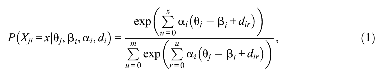In this model, three types of item parameters are estimated for an $m$ -category item: a discrimination or slope parameter, $α$ , and two parameters representing item difficulty: the location parameter, $β$ , and $m - 1$ category-specific threshold parameter, $d$ ( $\bar{d} = 0$ ).

P (X_{ji} = x | θ_{j}, β_{i}, α_{i}, d_{i}) = \frac{\exp (\sum_{u = 0}^{x} α_{i} (θ_{j} - β_{i} + d_{ir}))}{\sum_{u = 0}^{m} \exp (\sum_{r = 0}^{u} α_{i} (θ_{j} - β_{i} + d_{ir}))},

where

\sum_{r = 0}^{0} α_{i} (θ_{j} - β_{i} + d_{ir}) \equiv 0 .

This decomposition of the item difficulty in polytomous items has been referred to as extended parameterization (Penfield, Myers, & Wolfe, 2008). In contrast, the reduced parameterization (Masters, 1982) consists of $m - 1$ step parameters, $δ_{ir}$ , representing the intersections of two neighboring category response functions. both sets of item difficulty parameters can be transferred to one another by $δ_{ir} = β_{i} + d_{ir}$ . However, the choice of parameterization has implications for the interpretation of findings from invariance testing. Noninvariance with respect to $Δ_{ir}$ (reduced parameterization) pertains to between-group differences in advancing from one category to the next. Noninvariance under the extended parameterization affects between-group differences in an item’s overall difficulty ( $β_{i}$ ) and/or between-group differences with respect to one or more category-specific difficulties ( $d_{ir}$ ; Penfield et al., 2008). By disentangling the item difficulty, the extended parameterization provides useful insight into whether noninvariance is systematic for the entire item or specific to the step of advancing from one category to another.

In PISA 2015, three steps were performed to establish cross-group comparability. In a first step, a concurrent calibration using the GPCM was conducted in which all parameters were constrained to be equal across groups (languages within countries). In a second step, a group-specific item-fit statistic (RMSD) was calculated for each group and item and used as an indicator for the invariance of item parameters of an individual group. For a given latent construct, $θ$ , the RMSD statistic is calculated as

RMSD = \sqrt{\int {(P_{o} (θ) - P_{e} (θ))}^{2} f (θ) d θ},

quantifying the difference between the observed item characteristic curve (ICC; $P_{o} (θ)$ ) with the model-based ICC ( $P_{e} (θ)$ ), weighted by the $θ$ distribution (OECD, in press). It is sensitive to deviations of both the item difficulty and discrimination parameters (OECD, in press). RMSD ranges from 0 to 1, with larger values representing poorer item fit, thus indicating that the joint (“international”) parameters are not appropriate to describe the group’s data, that is, invariance does not hold. Item misfit was defined by cutoff values on the respective statistic: $RMSD > 0.1$ for the cognitive scales and $RMSD > 0.3$ for questionnaire constructs (OECD, in press). In case of item misfit for a given group, item constraints were released in a third step. Steps 1 to 3 were repeated until none of the groups exhibited misfit on any of the indicator items. Estimating group-specific (unique) item parameters in case of misfit resembles the concept of partial invariance (see above), assuming that the construct remains comparable when only a subset of indicator items receives unique item parameters.

In psychological research, attitudes are oftentimes assessed using a Likert-type response format. This study, therefore, examines the RMSD statistic’s behavior under known patterns of (non)invariance in polytomous items. Empirical distributions of this statistic across groups will provide insight into the appropriateness of different cutoff criteria for practical applications.

Method

Data Generation

In line with the scaling model used in PISA 2015, the GPCM (Equation 1) served as the true data generating model (OECD, 2016). Response data were generated for 1,000 simulees in 50 groups responding to five 4-category items. For four items $i$ , parameters were set to $β_{i} = 0$ , $α_{i} = 1$ , $d_{i 1} = - 1$ , $d_{i 2} = 0$ , and $d_{i 3} = 1$ . Each simulation condition (see below) was replicated 100 times. Within each replication, item parameters for Item 1 ( $β_{1}$ , $α_{1}$ ) as well as groups’ means ( $θ_{g}$ ) and standard deviations ( $σ_{θ_{g}}$ ) were drawn from the following distributions:

β_{1} ~ N (0, σ_{β}^{2}),

α_{1} ~ N (1, σ_{α}^{2}),

θ_{g} ~ N (0, 0.5),

σ_{θ_{g}} ~ U (0.8, 1.2) .

Simulation Design

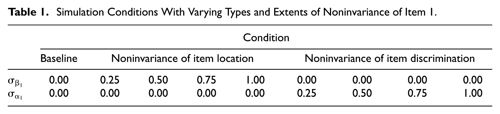
Both type and extent of noninvariance were manipulated between simulation conditions. The type of noninvariance was operationalized by drawing either the item locations $(β_{1})$ or the item discriminations $(α_{1})$ of Item 1 for the 50 groups from a normal distribution. As a result, one set of conditions represents noninvariance with respect to item location and one refers to noninvariance with respect to item discrimination. The extent of noninvariance was operationalized by manipulating the variation of these distributions: For each of the two parameters, the standard deviation was set to .25, .50, .75, and 1.0, respectively, while constraining the standard deviation of the other parameter to 0, resulting in a total of 2 (type) × 4 (extent) = 8 conditions. An additional baseline condition was simulated in which the parameters’ standard deviation was set to 0 for both parameters. This baseline condition represents the absence of cross-group parameter deviation, that is, the presence of invariance. It can serve as the control condition, representing the distribution that is expected under the null hypothesis (all groups have the same parameters). Table 1 provides an overview of the resulting nine simulation conditions.

Table 1.

Simulation Conditions With Varying Types and Extents of Noninvariance of Item 1.

	Condition
	Baseline	Noninvariance of item location				Noninvariance of item discrimination
$σ_{β_{1}}$	0.00	0.25	0.50	0.75	1.00	0.00	0.00	0.00	0.00
$σ_{α_{1}}$	0.00	0.00	0.00	0.00	0.00	0.25	0.50	0.75	1.00

Estimation Model

Following the scaling procedure used in PISA 2015, the simulated response data were scaled in a concurrent calibration with equal item parameters across all groups using the GPCM (Equation 1) in mdltm (von Davier, 2008). The RMSD statistic (Equation 3) was calculated for each group and item and aggregated across all 100 replications within each simulation condition. All analyses are based on these aggregated distributions of RMSD.

Results

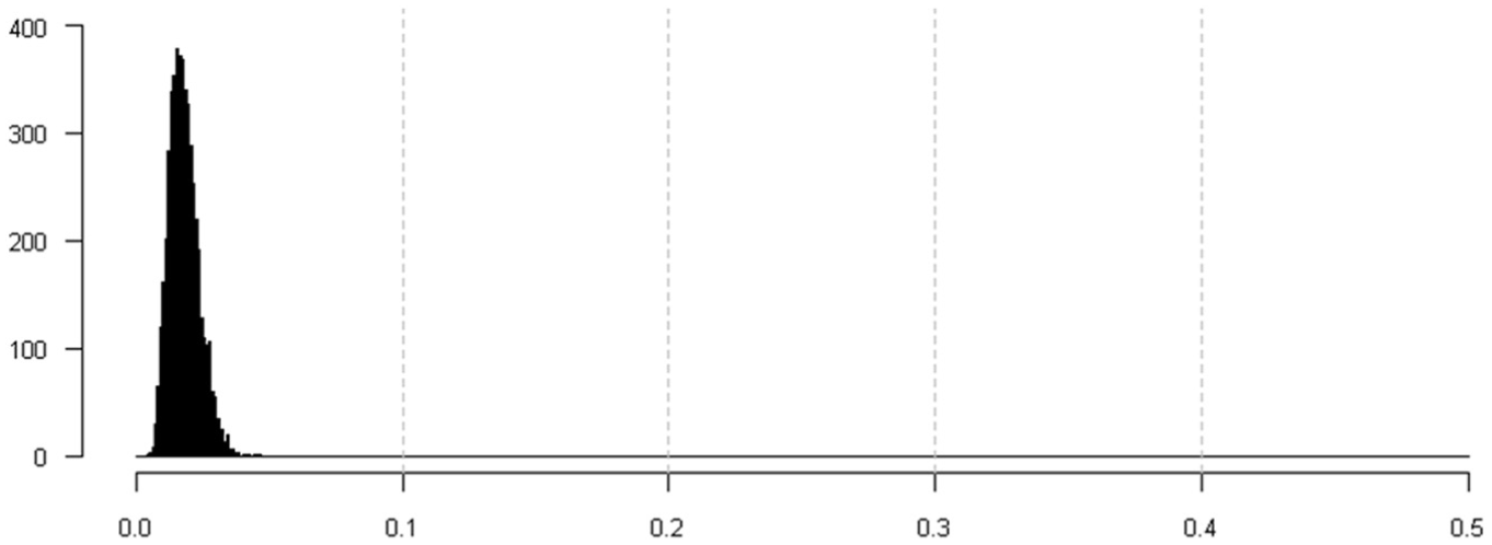
For each simulation condition, histograms indicating the RMSD distribution for Item 1 across all groups and replications are presented in the following. Figure 1 contains the respective distribution under the baseline condition ( $σ_{β_{1}} = 0, σ_{α_{1}} = 0$ ). The resulting distribution is skewed to the right, with the majority of values being very close to 0 ( $0.005 \leq RMSD \leq 0.047$ ).

Figure 1.

Distribution of RMSD for Item 1 across 50 groups and 100 replications in the baseline condition ( $σ_{β_{1}} = 0, σ_{α_{1}} = 0$ ).

Table 2 contains the respective plots for the eight remaining simulation conditions representing the conditions with noninvariant parameters. The x axes were held constant, ranging from RMSD values of .0 to .5. Tick mark labels on the x axes were omitted for simplicity, but vertical bars representing RMSD values of 0, .1, .2, .3, and .4 were retained. Similar to the baseline condition, all distributions are skewed to the right. However, within each type of noninvariance, the width of the RMSD distribution increases with increasing levels of the extent of noninvariance.

Table 2.

Distribution of RMSD for Item 1 Across 50 Groups and 100 Replications in Each Noninvariance Simulation Condition.

	Extent
Type	$σ_{β_{1}} = 0.25$	$σ_{β_{1}} = 0.50$	$σ_{β_{1}} = 0.75$	$σ_{β_{1}} = 1.0$
Item location (β)
	$σ_{α_{1}} = 0.25$	$σ_{α_{1}} = 0.50$	$σ_{α_{1}} = 0.75$	$σ_{α_{1}} = 1.0$
Item discrimination (α)

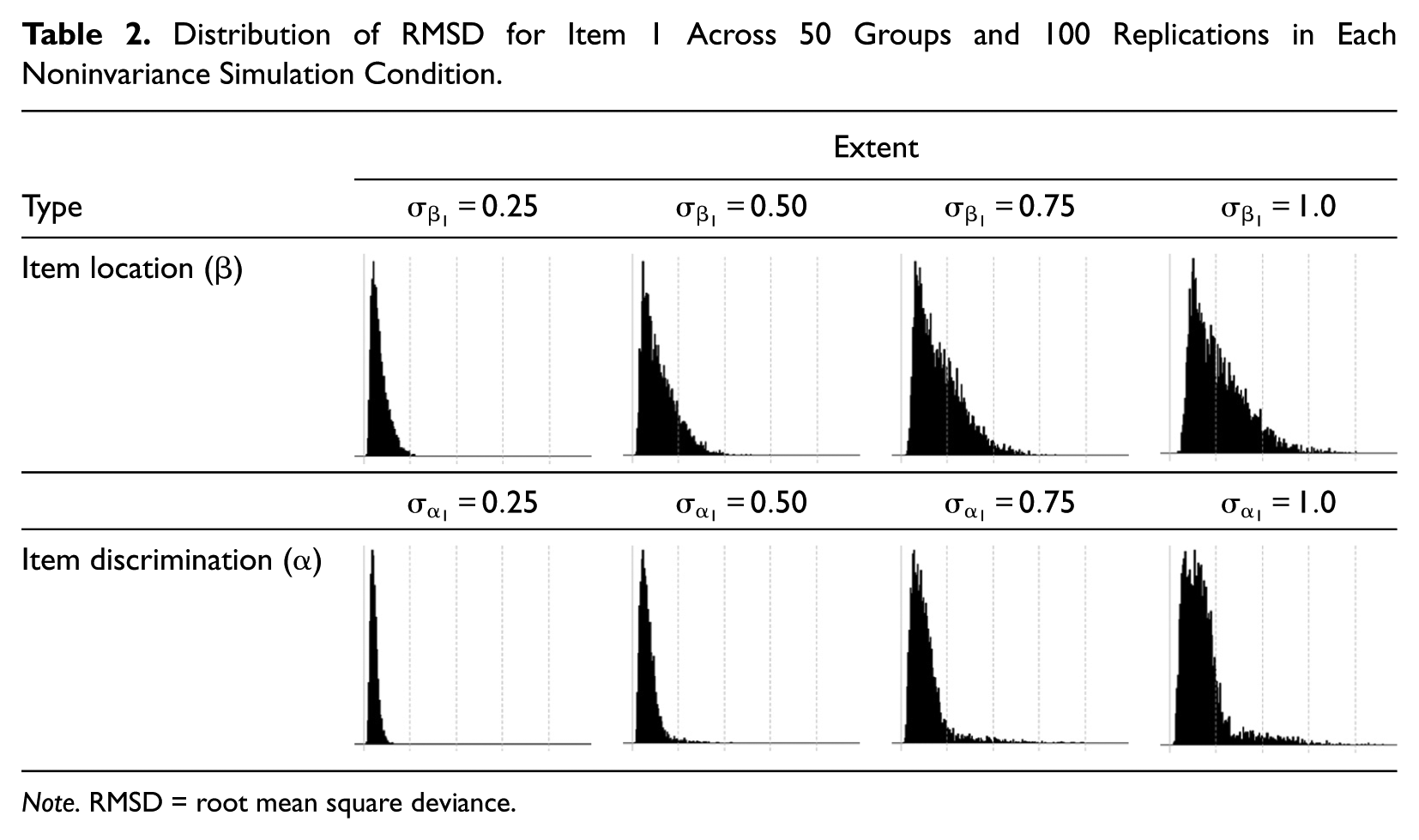
Note. RMSD = root mean square deviance.

In addition to the graphical display of findings, Table 3 provides descriptive statistics for the empirical RMSD distributions, covering minimum and maximum, 20th, 50th (median) and 90th percentile, and the proportion of cases exhibiting RMSD values above .1 and .3, respectively. Both minimum and maximum values increase as the extent of noninvariance increases. Similarly, increasing extents of noninvariance are associated with higher values for 50th and 90th percentile. The value associated with the 90th percentile can be interpreted as the RMSD value that separates the 10% of groups with the most extreme deviations from all other groups under a given true extent of noninvariance across groups. For example, the 10% of groups with the most extreme location parameters in the condition with the highest extent of noninvariance ( $σ_{β_{1}} = 1.0$ ) exhibit RMSD values of .188 or higher. The value with respect to the strongest variation in item discrimination ( $σ_{α_{1}} = 1.0$ ) is .126. Finally, the proportion of cases above RMSD values of .1 and .3 refer to the thresholds that were used in PISA 2015 to identify noninvariant items. The respective numbers in Table 3, therefore, may be interpreted as the proportion of items for which item parameters would have been released for individual groups, given the criteria used in PISA 2015. For example, 45.1% of items in the condition with the highest extent of noninvariance in item location ( $σ_{β_{1}} = 1.0$ ) and 16.5% in the condition with the highest extent of noninvariance in item discrimination ( $σ_{α_{1}} = 1.0$ ) would have been flagged as exhibiting noninvariance using the .1 criterion. It needs to be noted that in PISA 2015, this criterion was used to identify noninvariance in cognitive scales. A cutoff value of .3 was used to define noninvariance in the questionnaire constructs, thus corresponding to the data simulated in this study. When using this criterion, only about 1% of items would have been flagged for both types of noninvariance given the most extreme extents of noninvariance each.

Table 3.

Descriptive Statistics of RMSD for Item 1 Across 50 Groups and 100 Replications in Each Simulation Condition.

	Condition
	Baseline	$σ_{β_{1}}$				$σ_{α_{1}}$
		.25	.50	.75	1.00	.25	.50	.75	1.00
Minimum	.005	.006	.007	.013	.019	.006	.007	.007	.009
Maximum	.047	.148	.300	.334	.401	.101	.333	.396	.458
p20	.013	.020	.028	.040	.055	.016	.020	.028	.036
p50	.018	.030	.050	.073	.093	.021	.030	.045	.063
p90	.026	.060	.111	.153	.188	.033	.057	.091	.126
prop > .1	.000	.004	.136	.321	.451	.000	.025	.082	.165
prop > .3	.000	.000	.000	.001	.010	.000	.000	.003	.009

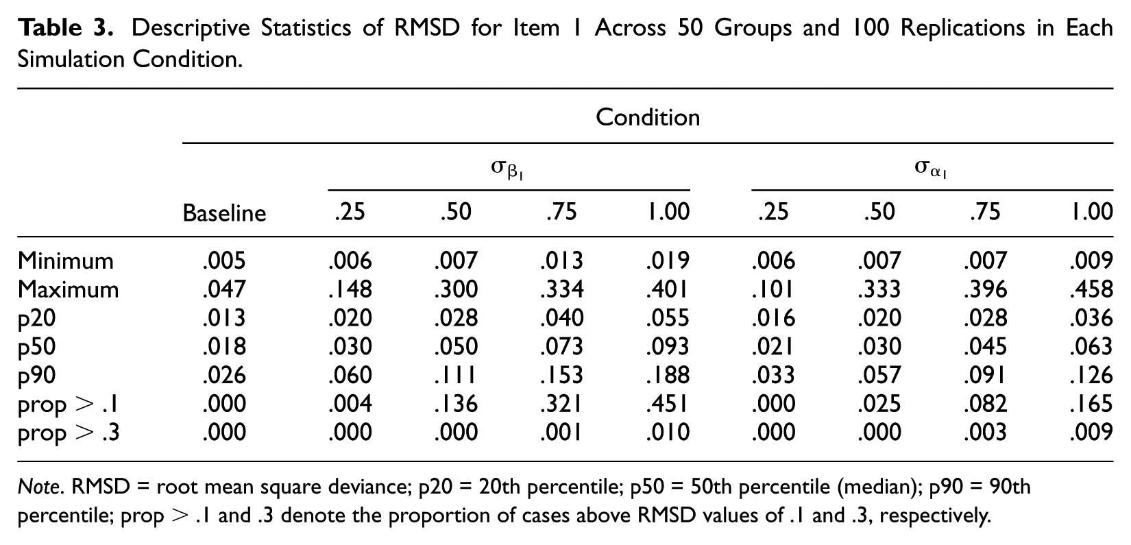
Note. RMSD = root mean square deviance; p20 = 20th percentile; p50 = 50th percentile (median); p90 = 90th percentile; prop > .1 and .3 denote the proportion of cases above RMSD values of .1 and .3, respectively.

With respect to the two types of noninvariance, findings indicate differential effects on RMSD depending on the noninvariant parameter. The same amount of cross-group variation in the location parameter is associated with larger RMSD values as compared with the discrimination parameter. This finding needs to be discussed in light of plausible ranges of location and discrimination parameters.

Discussion

This study examined an item-fit statistic, RMSD, which has recently been introduced as a measure of cross-country comparability of psychological constructs in a large-scale assessment context. The behavior of the statistic was investigated under known patterns of noninvariance across a large number of groups. Empirical distributions of the statistic provided insight into its range under specific conditions: either with respect to shifts in the general location of an item in the latent space, $β$ , or with respect to shifts in the item’s ability to discriminate between cases, $α$ .

Findings can be summarized according to three aspects: (a) RMSD is sensitive to between-group variability in both the item location and the item discrimination; (b) for each of these two parameters, RMSD is sensitive to the extent of between-group variability; and (c) the effect of between-group variability, measured in standard deviations, is larger for item location than it is for item discrimination. Care needs to be taken in the interpretation of the latter finding. In the two most extreme conditions (either $σ_{β_{1}} = 1$ or $σ_{α_{1}} = 1$ ), the $\pm 1 SD$ interval represents about 68% of the items:

- 1 \leq β_{1} \leq 1,

0 \leq α_{1} \leq 2 .

However, these intervals are on different scales and therefore have differential meanings. In this study, groups’ means and standard deviations were drawn, on average, from standard normal distributions (Equations 6 and 7). Therefore, the latent space where the majority of simulees are located corresponds to the general difficulty of the majority of items (Equation 8). The most extreme simulation condition relating to $β_{1}$ , therefore, denotes item difficulties that are not too uncommon. In contrast, the interval in which the majority of discrimination parameters are located given the most extreme simulation condition corresponds to discrimination parameters that are rather unusual in empirical applications (Equation 9). This simulation condition also implies an additional 16% of groups (i.e., eight groups per replication) that were assigned discrimination parameters of above 2. Moreover, another 16% (eight groups) received negative discrimination parameters. Taken together, the most extreme simulation condition with noninvariant discrimination parameters produced parameter values across groups that are rather unusual in practice while also demonstrating less of an impact on the RMSD distribution. Using cutoff values on RMSD is therefore more likely to flag items that vary with respect to item location than discrimination.

The present study can be used to inform setting a cut-score on RMSD, assuming that the distribution of parameters across groups corresponds to those implemented in this study. Table 3 contains the 20th percentile for each of the simulation conditions. For the noninvariance conditions, the respective value can be interpreted in terms of power, representing the point at which noninvariance is detected in 80% of cases. Referring to the most severe conditions for the two types of noninvariance, the respective RMSD values are .055 (location) and .036 (discrimination). To be more conservative, one could select RMSD = .055 as a cut-score. Being above the observed maximum in the baseline condition, this cut-score would also imply that no item or group is incorrectly flagged when invariance holds. Yet, as discussed above, this cut-score would detect noninvariance related to item discrimination ( $σ_{α_{1}} = 1.00$ ) in only about 58% of cases. It should be noted that these considerations are based on two rather extreme conditions of noninvariance, implying that the power to detect smaller violations of measurement invariance will be lower.

A strong assumption limiting the generalizability of findings is inherent in the simulation design of this study and relates to the way in which noninvariancebetween groups was simulated. When structuring traditional research on the topic, two branches can be differentiated, viewing groups as either fixed or random modes of variation (Muthén & Asparouhov, 2013). The first view assumes that the majority of parameters is the same across groups and relates to the question whether individual groups differ from all remaining groups. The second view assumes that parameters across groups are only approximately the same and focuses on the magnitude of variation between groups. In this simulation study, the authors operationalized noninvariance according to the second view, allowing parameters to show random variation. They thereby implicitly assumed that no individual country differs systematically from all other countries. However, such a situation may occur in the context of large-scale assessments, for example, in the case of a systematic translation error for one country or a set of homogeneous countries that changes the meaning of the measured construct from the one measured in all other countries. An additional simulation study may therefore focus on examining the RMSD’s capability to detect misfit that is systematic to a small subset of countries.

Going beyond the findings of this study, RMSD indicates between-group deviations in both location and discrimination parameter, thus not informing about the actual cause of noninvariance. Possible causes could be group differences with respect to discrimination, general item difficulty (location), the difficulty of individual response options (step parameters or thresholds), or even a mixture of some or all of the above. As a result, both location and discrimination parameters were released for a group’s item in PISA 2015 as soon as this item exhibited misfit. A further development in IRT-based invariance testing could make use of the stepwise approach in MGCFA in which sets of parameters are constrained and differences in model fit are monitored. Similarly, the different parameters in an IRT model could be released one after another and differences in item fit could be tracked using the RMSD statistic. Similar to MGCFA, item difficulty parameters may be released before item discrimination. Such a procedure promises a higher level of comparability across groups while revealing some information about the cause of between-group differences. Such an approach could be subject to further research, as well as the performance of RMSD for detecting differences in threshold parameters. Disentangling cross-group differences in an item’s general difficulty from relative difficulties of particular response options promises valuable insights in applied contexts.

Footnotes

Declaration of Conflicting Interests

The author(s) declared no potential conflicts of interest with respect to the research, authorship, and/or publication of this article.

Funding

The author(s) received no financial support for the research, authorship, and/or publication of this article.

ORCID iD

Janine Buchholz

References

Byrne

B. M.

Shavelson

R. J.

Muthén

(1989). Testing for the equivalence of factor covariance and mean structures: The issue of partial measurement invariance. Psychological Bulletin, 105, 456-466.

Cieciuch

Davidov

Schmidt

Algesheimer

Schwartz

S. H.

(2014). Comparing results of an exact versus an approximate (Bayesian) measurement invariance test: A cross-country illustration with a scale to measure 19 human values. Frontiers in Psychology, 5, 1-10. doi:10.3389/fpsyg.2014.00982

Dimitrov

D. M.

(2010). Testing for factorial invariance in the context of construct validation. Measurement and Evaluation in Counseling and Development, 43, 121-149.

Fox

J.-P.

Verhagen

A. J.

(2010). Random item effects modeling for cross-national survey data. In Davidov

Schmidt

Billiet

(Eds.), Cross-cultural analysis: Methods and applications (pp. 467-488). London, England: Routledge.

Holland

P. W.

Thayer

D. T.

(1988). Differential item performance and the Mantel-Haenszel procedure. In Wainer

Braun

H.I.

(Eds.), Test validity (pp. 129-145). Hillsdale, NJ: Lawrence Erlbaum.

Jöreskog

K. G.

(1971). Statistical analysis of sets of congeneric tests. Psychometrika, 36, 109-133.

Masters

G. N.

(1982). A Rasch model for partial credit scoring. Psychometrika, 47, 149-174.

Mellenbergh

G. J.

(1989). Item bias and item response theory. International Journal of Educational Research, 13, 127-143. doi:10.1016/0883-0355(89)90002-5

Meredith

(1993). Measurement invariance, factor analysis and factorial invariance. Psychometrika, 58, 525-543. doi:10.1007/BF02294825

10.

Muraki

(1992). A generalized partial credit model: Application of an EM algorithm. Applied Psychological Measurement, 16, 159-176.

11.

Muthén

Asparouhov

(2013). New methods for the study of measurement invariance with many groups. Retrieved from http://statmodel2.com/download/PolAn.pdf

12.

Organisation for Economic Co-Operation and Development. (2016). PISA 2015 results (volume I): Excellence and equity in education. Paris, France: Author. doi:10.1787/9789264266490-en

13.

Organisation for Economic Co-Operation and Development. (in press). PISA 2015 technical report. Retrieved from http://www.oecd.org/pisa/data/2015-technical-report/

14.

Penfield

R. D.

Myers

N. D.

Wolfe

E. W.

(2008). Methods for assessing item, step, and threshold invariance in polytomous items following the partial credit model. Educational and Psychological Measurement, 68, 717-733.

15.

Raju

N. S.

van der Linden

W. J.

Fleer

P. F.

(1995). IRT-based internal measures of differential functioning of items and tests. Applied Psychological Measurement, 19, 353-368.

16.

Reise

S. P.

Widaman

K. F.

Pugh

R. H.

(1993). Confirmatory factor analysis and item response theory: Two approaches for exploring measurement invariance. Psychological Bulletin, 114, 552-566.

17.

Rutkowski

Svetina

(2014). Assessing the hypothesis of measurement invariance in the context of large-scale international surveys. Educational and Psychological Measurement, 74, 31-57.

18.

Swaminathan

Rogers

H. J.

(1990). Detecting differential item functioning using logistic regression procedures. Journal of Educational Measurement, 27, 361-370. doi:10.1111/j.1745-3984.1990 .tb00754.x

19.

van de Schoot

Schmidt

De Beuckelaer

Lek

Zondervan-Zwijnenburg

(2015). Editorial: Measurement invariance. Frontiers in Psychology, 6, Article 1064. doi:10.3389/fpsyg.2015 .01064

20.

von Davier

. (2008). A general diagnostic model applied to language testing data. British Journal of Mathematical and Statistical Psychology, 61, 287-307.

21.

Zumbo

B. D.

(2007). Three generations of differential item functioning (DIF) analyses: Considering where it has been, where it is now, and where it is going. Language Assessment Quarterly, 4, 223-233.

Comparing Attitudes Across Groups: An IRT-Based Item-Fit Statistic for the Analysis of Measurement Invariance

Abstract

Keywords

Introduction

Different Approaches to Testing Measurement Invariance

The Root Mean Square Deviance (RMSD) Item-Fit Statistic

Method

Data Generation

Simulation Design

Estimation Model

Results

Discussion

Footnotes

Declaration of Conflicting Interests

Funding

ORCID iD

References