Sage Journals: Discover world-class research

Abstract

Applying a recently developed framework for the study of sample-based person impressions to the level of group impressions resulted in convergent evidence for a highly robust judgment process. How stimulus traits mapped on the resulting group impressions was subject to two distinct moderators, diagnosticity of traits, and the amplifying impact of early sample truncation. Three indices of diagnosticity—negative valence, extremity, and distance to other traits in a density framework—determined participants’ decision to truncate trait sampling early and hence the final group judgments. When trait samples were negative and extreme and when the distance between high-density traits was small, early truncation of the trait samples fostered high group homogeneity and polarized impressions. Granting that mental representations of in-groups and out-groups rely on systematically different samples, our sampling approach can account for various inter-group biases: out-group homogeneity, out-group polarization and (because negative traits are more diagnostic) out-group derogation.

Keywords

out-group homogeneity out-group polarization self-truncated sampling diagnosticity

Out-group homogeneity (or relative in-group heterogeneity) is a classical and intensely discussed finding in social cognition and inter-group research. The concept points to divergent mental representation of groups we are part of (in-groups) and of groups we do not belong to (out-group). Specifically, the variability between individuals and target behaviors is perceived to be lower for out-groups such as a rival university, another age group or a foreign culture than for in-groups such as one’s own university, age group, or culture (Linville et al., 1989; Quattrone & Jones, 1980).

Theoretical explanations of this asymmetry vary on a continuum, one pole of which emphasizes structural causes in the environment whereas the other pole emphasizes motives and conflicts within the individual. Structural causes typically reflect the different sample (Kareev et al., 2002; Konovalova & Le Mens, 2020; Linville et al., 1989; Linville & Fischer, 1993) and unequal knowledge (Park & Rothbart, 1982) about in-groups compared with out-groups. Motivational accounts, in contrast, stress the desire to develop a positive in-group identity (Simon & Brown, 1987) along with optimal distinctiveness (Brewer, 1993) and the familiarity advantage of closer individuals. Although there can be no doubt that motivational biases, real conflicts, group-related emotions, or xenophobia are sufficient to trigger inter-group biases, a controversial question is whether they represent necessary conditions. Proponents of cognitive ecological theory perspectives have pointed out that biased judgments and decisions can originate in completely unbiased intrapsychic processes (Denrell & Le Mens, 2007; Fazio et al., 2004; Fiedler, 2000; Fiedler & Wänke, 2009) embedded in perfectly adaptive behavior. Even when all stimuli are processed the same way, whether they are positive or negative in valence and related to in-groups or out-groups, the resulting judgments or evaluations can exhibit a systematic bias, simply because the stimulus environment imposes unequal samples of in-group or out-group related information on our mental representations. One obvious source of inequality is sample size, which is the focus of the present research. Because our own group membership creates more opportunities to observe behaviors of in-group members in comparison to out-group members’ behaviors, it seems self-evident that we are exposed to larger samples of in-group than out-group information (Bergh & Lindskog, 2019; Quattrone & Jones, 1980).

Aim of the Present Investigation

The aim of the present investigation is to outline a sampling-theoretical approach to the study of inter-group relations. The purpose of the first experiment is to establish the paradigm and to demonstrate that the same trait-sampling process that we have shown in previous publications on individual impression formation also apply to the formation of group impressions (Prager et al., 2018; Prager & Fiedler, 2021). Two pre-studies are devoted to scale materials for subsequent testing of two presuppositions of this approach. First, the same basic sampling phenomena and the same inter-group findings (out-group homogeneity and out-group derogation) are obtained regardless of whether group labels are meaningful and related to existing social groups or whether meaningless group labels are used. Second, we demonstrate that (group) impressions are not merely a function of the size of trait samples, but of the diagnosticity of traits. In the spirit of the density model (Unkelbach et al., 2008), we focus on two stimulus-inherent aspects of diagnosticity, (negative) valence and extremity of traits, and on within-sample density (i.e., similarity) as a major source of internally determined diagnosticity. To elucidate the underlying mechanism, we elaborate on possible sufficient conditions to the two major inter-group phenomena (out-group homogeneity and out-group derogation).

Sample Size and Inter-Group Relations

A review of previous research suggests two different explanations of why small sample size may be at the heart of out-group homogeneity. The first explanation can be derived from statistical sampling theory, as formalized in Linville et al.’s (1989) seminal work. The loss of one degree of freedom in the calculation of a sample variance implies a systematic variance reduction for small samples (when n−1 is markedly smaller than n) than for large samples (when n−1 approximates n). The resulting decrease in actual variance with decreasing n was shown by Kareev et al. (2002) to account for a sizable part of judgment biases.

In contrast to this formal statistical proof, a second explanation attributes the reduced variance of smaller samples to a “hot-stove” effect (Denrell, 2005). Assuming that adaptive agents tend to repeat pleasant and stop unpleasant behaviors (Thorndike, 1927), they will under specifiable conditions (Denrell, 2005; Denrell & Le Mens, 2007) truncate sampling from negative sources while continuing to sample from pleasant sources. Consequently, they forego the possibility to correct for initial negativity effects, having only a chance to correct for initially inflated positive impressions (leading to larger samples of moderately positive stimuli). This explanation attributes both the perceived homogeneity and the derogation of small samples to the agent’s hedonic sampling strategy (Thorndike, 1927), which is neither irrational nor driven by any motivated bias against some stigmatized target (Le Mens & Denrell, 2011).

Self-Truncation Effects

The mechanism proposed in the present research is categorically different from those of earlier accounts. It can neither be reduced to the statistical (n−1)/n correction that underlies Linville’s work nor does it reflect a hot-stove effect of the kind proposed by Fazio et al. (2004) or by Denrell and Le Mens (2007). It is rather based on recent findings uncovered in our own research on impressions of individual targets based on samples of traits (Prager et al., 2018; Prager & Fiedler, 2021). Across a series of experiments, we found that, as long as sample size was an experimentally determined independent variable, the strength (extremity) of judgments increased with increasing samples of traits. When however, participants in a self-truncated sampling condition could themselves stop sampling when they felt ready to judge, the strength of judgments bore a clearly negative correlation to sample size. Self-truncated sampling introduces the possibility to exploit instances of the first few items to exhibit a strong, presumably stable, conflict-free and consistent trend and to stop sampling at an early stage. In contrast, sample size is increased when no such initial strong trend occurs. As a consequence, self-truncated sampling regularly produces small-sample polarization patterns.

Diagnosticity Amplifies Self-Truncation Effects

This basic consequence of self-truncated sampling depends strongly on the diagnosticity of the sampled stimuli. Not every stimulus item is equally likely to influence the resulting group judgment and not every item is equally likely to facilitate truncation. The likelihood to truncate a sample increases when the first few items in a sample are high rather than low in diagnosticity. Traits are more diagnostic if they are extreme rather than moderate and if they are negative rather than positive (Prager et al., 2018; Reeder & Brewer, 1979; Rothbart & Park, 1986; Skowronski & Carlston, 1987). Thus, the negative relationship between sample size and the tendency to solicit strong judgments is more pronounced when negativity and extremity render stimuli diagnostic.

Density Model

The density hypothesis (Unkelbach et al., 2008) offers a deeper understanding of the cognitive underpinnings of the diagnosticity concept and the way it moderates adaptive cognition. Positive stimuli are closer to each other and more densely interconnected in associative memory than negative stimuli, which are more distinct in meaning and less overlapping. For example, people who are polite are also very likely friendly and punctual and reliable and tactful. In contrast, if people are dishonest, we can hardly infer that they are offensive, brutal, depressed, or resentful. Whereas positive person attributes form interconnected clusters, producing integrative halo effects (Unkelbach et al., 2008), negative attributes denote more separable properties. Thus, positive person attributes are common and redundant, whereas negative attributes are distinct, particular, and diverse.

At the behavioral level, positive words can be recognized and verified faster than negative stimuli (Unkelbach et al., 2008), because high-density clusters of positive stimuli in associative memory allow for a good deal of parallel processing. For the same reason, though, single positive words or person attributes add little to the semantic meaning of other positive items in the cluster, and a higher rate of positive evidence is required to confirm a positive judgment (Gidron et al., 1993; Rothbart & Park, 1986). Recognizing and confirming negative words and attributes takes longer but exerts stronger impact on evaluative judgments. Negative valence is, thus, a major determinant of diagnosticity, and the density model offers a mental account (i.e., the unequal distance and overlap or positive and negative stimuli in memory) and a reasonable measure of diagnosticity (i.e., the average distance from the remaining stimuli in a set, measured through multidimensional scaling; see Koch et al., 2016).

Yet, negative valence is by no means the only determinant of diagnosticity. Pitting diagnosticity against valence, it has been shown that those exceptional negative stimuli that bear low distances to others behave like high-density (non-diagnostic) stimuli and exceptional positive stimuli with high distances to others behave like low-density (diagnostic) stimuli (Unkelbach et al., 2008). Because extreme stimuli are also more distant from other stimuli, they were found by Prager et al. (2018; see also Fiske, 1980) to exert stronger influence on growing impressions than moderate stimuli. Drawing on the density model as a conceptual tool, we, therefore, expect stronger self-truncation effects resulting in stronger impression judgments for negative than positive traits, and for extreme than moderate traits.

Preview and Predictions

We expect the typical self-truncation effects (i.e., negative correlation between self-truncated sample size n and judgment strength J¹) to carry over from individual to group impressions. This basic prediction is not trivial. Because every trait in the group impression formation task refers to a different individual, entitativity is lower for groups than for individuals (Campbell, 1958; Yzerbyt et al., 2000). To capture the impact of entitativity, we compare impressions of groups with familiar and meaningful labels with neutral groups with meaningless labels.

In our previous research on individual-target impression formation, we regularly found that truncated sampling produces negative correlations r_n,J between sample size and judgment strength (Prager & Fiedler, 2021; Prager et al., 2018). Parallel to this small-sample polarization effect, we hypothesize negative correlations r_n,H between sample size and judgment strength. The tendency to judge small, early truncated samples (groups) more homogeneous and more extreme increases with diagnosticity, as manipulated by the selection of traits. Although out-group homogeneity and out-group polarization are immediate consequences of self-truncated sampling, out-group polarization can be shifted to out-group derogation by the higher diagnosticity of negative than positive information. The moderating effect of diagnosticity on self-truncated sampling results in a noticeable asymmetry in sample truncation and judgments, causing especially initially negative samples to be stopped at small sample size and to be judged more extremely.

This outline should reveal what is theoretically novel and original about the present approach. The depicted self-truncation mechanism can be neither reduced to the statistical (n−1)/n argument that motivated Linville et al.’s (1989) approach, which in turn cannot account for the persistent negative correlations r_n,J and r_n,H. Nor can it be considered a special case of a hot-stove effect leading to a one-sided negativity bias, because self-truncation effects are not restricted to hedonic avoidance of negative outcomes. We also go beyond previous research by specifying and testing the impact of diagnosticity. Our sample-based judgment approach offers a sensible account for several prominent inter-group biases: out-group homogeneity, out-group polarization, and out-group derogation, and for the co-occurrence of these major biases. Though self-truncation effects were already demonstrated for judgments of individual targets, placing them in the context of inter-group theorizing yields a variety of novel insights, about inter-group biases and downstream consequences of self-truncation.

Stopping Rules Underlying Sample Truncation Algorithms

Why does early truncation render small samples more extreme and more homogeneous than large samples? Granting that small samples are more likely to produce extreme values in terms of all four moments—means, variance, skewness, and curtosis—it seems plausible on intuitive grounds that (inter-group) biases are more pronounced for small than for large samples. Going beyond intuition, it is certainly appropriate to look out for a formal solution. The pertinent literature, indeed, suggests two algorithmic models, which converge in predicting stronger outgroup homogeneity (inverse of sample standard deviation [SD]) and stronger that judgment strength (J) when n increases, although they rely on different assumptions. The first model, based on a simplified n-dependent stopping rule, was proposed by Haldane (1945). The second model uses an n-independent Bayesian stopping rule that relies on updating a beta-distribution.

Haldane’s Labor-Saving Sampling Method

Assuming that judges, like statisticians, are sensitive to sample size n, Haldane (1945) proposed the standard error se as a variable threshold, predicting sample truncation when the number k of “likeable” traits (or the complementary number n−k of “non-likeable” traits) in a sample of n exceeds an a-priori chosen threshold t. Such a stopping rule implies that sample heterogeneity (conceived as inverse standard deviation SD) increases with sample size n, because SD = se_t * √n (see left chart in Figure 1) while impression strength J decreases with increasing n (see right chart).² Note that a positive J reflects a deviation of judgments from .5 in the correct direction.

Figure 1.

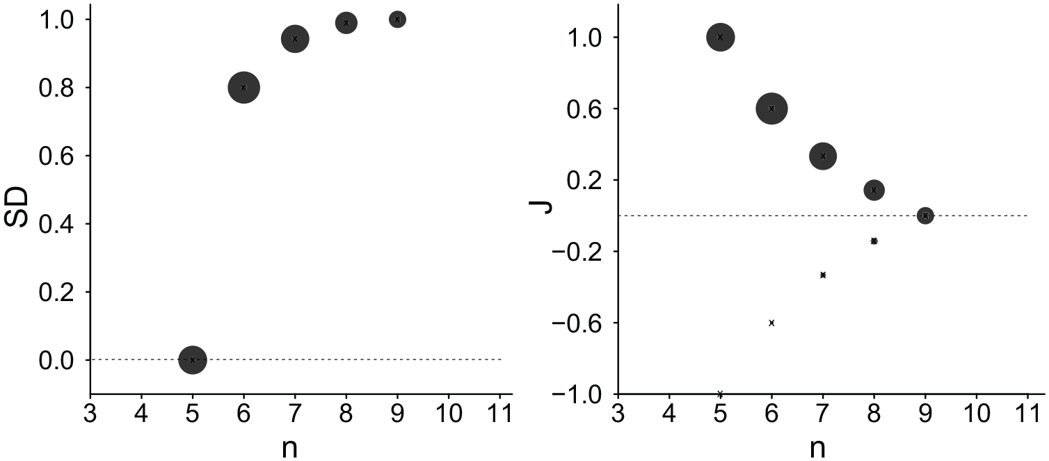
Simulated Sample SD (Inverse of Homogeneity; Left Chart) and Judgment Strength J (Right Chart) as a Function of n, the Size of Samples Truncated by Haldane’s (1945) Rule, Assuming a True Likeability Probability of p(“likeable”) = .75 and a Threshold of t = 5.

Belief-Updating Using the Beta-Distribution in Sample-Based Impressions

A Bayesian approach, in contrast, stopping the sample becomes evidence dependent, and essentially independent of sample size $n . In$ Bayesian calculus, the posterior odds of, say, p(“likeable”| all sampled traits) / p(“unlikeable”| all sampled traits) equals the prior odds (set to 1:1 for uniform priors) multiplied k times with a likelihood ratio of LR = p(likeable trait added | “likeable” group) / p(likeable trait added |“unlikeable” group) and (n−k) times with the reverse ratio 1/LR. Because k LR updates and (n−k) 1/LR updates cancel each other out, a Bayesian stopping rule is sensitive to the frequency difference, not the ratio, of likeable and unlikeable members. Thus, the same 2:1 ratio of 16 likeable and 8 unlikeable traits in a larger sample affords stronger evidence for the prevailing positivity than 8 likeable and 4 unlikeable traits.

We realize uniform priors as a beta distribution $B e t a (α = 1, β = 1),$ assuming that every possible value appears equally likely before any evidence is observed. Updating these priors with k “likeable” and $(n - k)$ “non-likeable” traits, the posterior probability density distribution becomes $B e t a (α_{0} + k, β_{0} + n - k) .$ ³ Sampling is truncated when the highest density of this posterior distribution is condensed within a sufficiently narrow interval. The width of this interval is an expression of how confident and stable the current impression is. Truncating samples this way produces similar (increasing) SD and (decreasing) J functions of n as the Haldane algorithm (Figure 2). Thus, whether the stopping rule is sensitive to n or not, the simulated self-truncation effect on homogeneity and extremity of group impressions remains largely invariant. They corroborate the notion that both J (judgment strength and the inverse of SD (homogeneity) decrease with increasing sample size n. Granting that larger samples represent in-groups and smaller samples represent out-groups, both simulations converge in predicting out-group homogeneity as well as out-group polarization: Self-truncated small samples are regularly more homogeneous (consistent, conflict-free) and lead to stronger (more polarized) judgments than larger, non-truncated samples.

Figure 2.

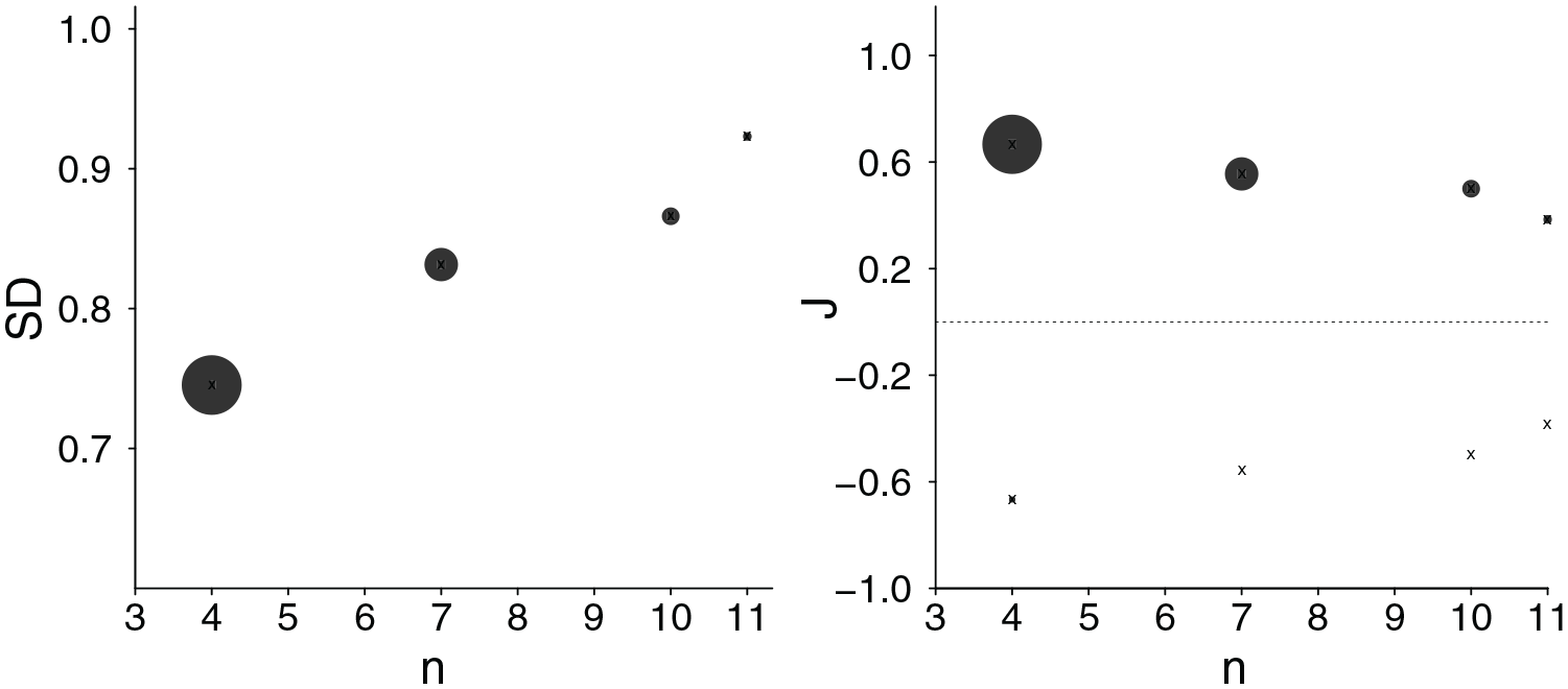
Plot of Sample SD (Left Chart) and Judgment Strength J (Right Chart) as a Function of n, the Size of Samples Truncated According to a Bayesian Stopping Rule, Assuming Truncation When 90% Posterior Highest Density Becomes Narrower Than the Threshold Interval Width t = .4.

Empirical Evidence

Encouraged by these simulation results and by converging evidence from earlier simulations and experiments (Prager et al., 2018; Prager & Fiedler, 2021), the purpose of our empirical research was to illuminate the antecedents (determinants of diagnosticity) and the consequences (homogeneity, and judgment strength) of self-truncated trait samples. Our main experiments (Experiments 1–3) aimed at demonstrating that the same trait-sampling processes that govern individual impression judgments can be generalized to group impression formation, when each new trait represents another group member. The analogy of individual and group impression formation holds in particular for the accentuating impact of self-truncation. In preparation of Experiment 1, we ran a first pre-study to scale labels of commonly known social groups. A second pre-study then established the applicability of the density model to the traits used in the following experiments, using a method introduced by Goldstone (1994).

Pre-Study 1: Sample Size, Homogeneity, and Evaluation of Existing Social Groups

We selected labels of 28 social groups from Study 3a in Koch et al. (2016), for example “artists,” “car drivers,” “conservatives,” or “vegans.” We selected groups that were supposedly familiar to most people (see Appendix). Two subsets of participants were asked to rate either group knowledge (N = 119) or group likeability and homogeneity (N = 83). Group labels were presented one after another. After seeing a new group label, knowledge ratings were prompted by two questions (on the same screen below the displayed label): “How much do you know about this group in general?” and “How many members of this group do you know?” They responded by clicking on continuous scales below each question, the endpoints of which were “nothing” versus “very much,” “none” versus “a great many,” respectively. A second subset of participants rated groups for likeability and homogeneity, prompted by the questions “How much do you like this group?” (continuous scale, endpoints labeled “strong antipathy” and “strong sympathy”) and “How similar are group members to each other?” (endpoints “very different” and “very similar”).

Results and Discussion

We averaged responses to both knowledge questions, which were highly correlated (individual correlations per participant: Mean r = .77, SD = .18; individual correlations were positive for 99% of all participants). Group ratings of likeability and homogeneity ratings for each social group were averaged across participants. Taking the self-reported amount of knowledge as a proxy of the size of the information sample, we assessed the ecological effect of small-sample derogation and homogeneity. As expected, the amount of group knowledge correlated positively with likeability ratings, r = .42, t(26) = 2.38, p = .025, and inversely with homogeneity ratings, r = −.58, t(26) = 3.62, p = .001. Thus, an increasing amount of knowledge on a group came along with higher likeability and lower perceived within-group homogeneity.

Pre-Study 2: Density of Traits

The second pre-study served to validate the assumption that density (i.e., average distance to other stimuli) is higher for positive than for negative traits, and for extreme than for moderate traits. Thus, diagnosticity should be higher for low-density than for high-density traits. As explained above, especially the asymmetry between positive and negative traits forms the basis of shifting the small-sample polarization toward a small-sample derogation effect.

Method

The stimulus traits were a set of 70 adjectives that had been scaled for valence in Prager and Fiedler’s (2021) experiments on individual impression formation. Using the spatial arrangement method (Goldstone, 1994), we assessed the distance between traits as the core feature of density. In each round, participants were asked to position 12 randomly selected traits (font size 24 pt) in a white square (side length 278 px). They were instructed to group fitting words together and to spatially separate non-fitting ones. The white square was initially empty; participants could then drag and drop traits one after another from a gray box below the positioning area by clicking, moving and releasing the mouse. Traits could be relocated later. After all 12 items were placed, participants cleared the screen and initiated a new round of 12 traits by clicking a button. For each round, the 12 traits were drawn randomly without replacement from the entire pool of traits. The order of traits was newly randomized for each participant.

The age of the 95 participants ranged from 18 to 65 years (M = 24.93), with 78 being female, 16 male, and 1 of other gender. Ninety participants were students (16 psychology students). The whole procedure was executed by Java software. For each possible pair out of the set of 70 traits, the Euclidean distance between placement positions was averaged across all participants who rated that pair of traits.

Results

For each trait, we calculated the density as the sum of squared distances to all other traits in the set. Going beyond Unkelbach et al. (2008), we not only expected negative traits to be more distant from other traits compared with positive ones but also extreme traits to be more distant from others than moderate ones. In a regression analysis of distance scores, this two-fold expectation should be evident in a strong valence effect, represented by a linear trend (i.e., distance decreasing with trait positivity) along with an extremity effect in form of a quadratic trend (to capture the higher distance of extreme than moderate traits of either valence). Figure 3 corroborates exactly this pattern. Standardized regression coefficients confirmed that low-distance (i.e., high-density) traits were systematically more positive, linear β = −.64, t(68) = 6.84, p < .001, and less extreme than high-distance traits, quadratic β = .21, t(68) = 2.28, p = .026.

Figure 3

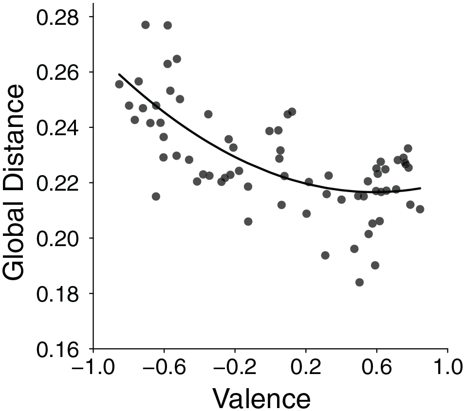
Average Pairwise Distance Between Each Trait and All Other Traits of the Remaining Set (i.e., “Global Distance”) Plotted as a Function of Trait Valence Norms.

Experiment 1

Having approved the stimulus materials, we can move on to the main experiments. In essence, we wanted to demonstrate that similar self-truncation effects as in former research by Prager et al. (2018) on impressions of individual targets can be found in a group impression formation task of clearly less entitativity, when each sampled trait refers to a different group member. Moreover, because inter-group research is concerned with both homogeneity and impression strength, we assessed both group likeability and group homogeneity using two operationally independent measures: rating scales and the distribution-builder method, as explained in the “Method” section below. We expected judgments of group homogeneity and polarization (on the likeability scale) to be not only determined by the traits sampled from the population set but also by the impact of self-truncation.

Method

To substantiate the assumption that group impressions, like individual impressions, are mainly determined by a sample of n traits, we compared one condition with meaningful labels of existing social groups to another condition with meaningless labels (“Group A”), which should similarly depend on the stimulus sample of n traits. Based on materials constructed in previous research (Prager & Fiedler, 2021) on individual impression formation, we relied on population sets of traits that represented different levels of diagnosticity (valence and extremity). Stimulus samples in all four experiments were randomly drawn from these sets.

Estimation of Statistical Power

In this and the following experiments, we aimed at a minimum participant sample of N = 80. We conducted a power analysis by using a Monte-Carlo simulation. For convenience, we rely on bivariate correlation coefficients as effect size estimates, calculated within each participant across all trials. We test these individual correlations against 0. For a minimum trial number of 20 (Experiment 2) and the minimum participant sample size of N = 80, ρ = .09 is the minimum effect size that can be reliably (α = .05) detected with power 1−β = .95.

Participants and Design

One-hundred and thirty-four participants were recruited from a participant pool at Heidelberg University. Participants’ age ranged from 17 to 77 (M = 24.88); 107 participants were female. One hundred and twenty-six participants were students, of which 36 were students of psychology. The experiment (realized as a Java program) was embedded in a sequence of four unrelated studies (on directed forgetting, speed-accuracy trade-off, and simultaneous encoding of two trends) at a Heidelberg University laboratory. Participation in the study series, which lasted about 60 min, was compensated either by payment (8€) or by course credit. Fifteen participants who had invariantly sampled only one or all 16 traits on every trial were excluded. Of the remaining participants, 62 were randomly assigned to the Meaningful Group Labels Condition and 57 to the Meaningless-Labels Condition. The positivity proportion p of the population set from which trait samples were drawn within participants as a repeated-measures factor. The major dependent measures, likeability (L) and homogeneity (H) of groups were assessed in two operationally independent ways, using the distribution builder and rating scales.

Materials

From the pooled list of 70 adjective traits (see pre-study), we extracted four partly overlapping population sets of 30 stimulus traits, from which the stimulus samples were drawn. The four population sets had positivity proportions of p = .20, .33, .67, .80⁴; that is, two sets were predominantly positive, two negative in valence and orthogonally, two sets were of moderate and two of extreme valence. On each trial, a target group was described by a newly drawn random sample of traits from one population set. Each participant completed 28 trials in random order, seven drawn from each population set.

Procedure

Participants received instructions saying that each trial started with a group label displayed on top of the screen (21pt boldface). By pressing the space bar, participants could invoke a new trait (displayed in font size 20pt in the top center region of the screen). At each point between n = 1 and n = 16, they could choose to either solicit another trait (by pressing the space bar again) or to truncate the sample using the Enter key and proceed to the judgments. All traits remained on screen as long as sampling continued. Traits were listed vertically; when sample size exceeded n = 8, additional traits were displayed in a second column. The most recent trait was highlighted by enhanced contrast.

Immediately after the truncation of a sample, participants provided their group judgments. Using a modified version of the Sharpe et al. (2000) “distribution builder,” they were asked to construct a distribution for the group’s likeability, by clicking the cells of six degree-of-liking columns of a 6×6 grid (illustrated in Figure 4). Clicking a cell in a column resulted in placement of a gray square in the respective column. Note that the distribution builder offers a measure of both the mean and dispersion of the likeability impression on the target group.

Figure 4.

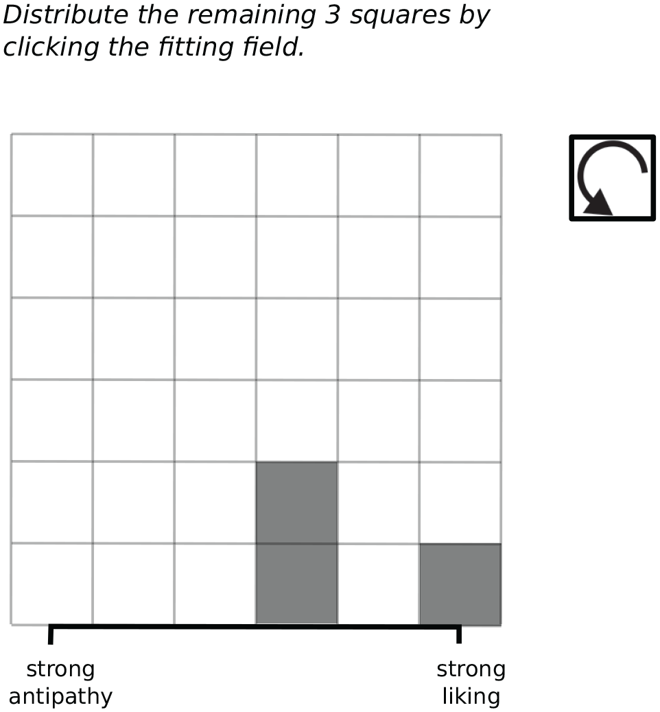
Distribution Builder: A Participant Has Already Placed Three Squares on a Moderately and an Extremely Positive Likeability-Position.

Upon completion of the distribution builder task, participants continued to a new screen on which three horizontal graphical rating scales with marked endpoints appeared one after another. They provided their ratings by clicking on the appropriate horizontal scale position. Scales referred to likeability, L, (“How much would you like that group” with endpoints “highly unlikeable” and “highly likeable”), homogeneity, H, (“How similar are the group members in their likeability?,” endpoints “very different” to “very similar”), and confidence C in both ratings (“How confident are you in these judgments?” ranging from “very uncertain” to “very sure”). During the judgment phase, the current group label remained visible in the central top position on the screen. After completing all ratings, participants could start a new trial by clicking a button,⁵ with a new group label indicated on top and a new sample of traits.

Results

Quality of Judgment Data

Table 1 provides an overview of the reliability of the judgment data from all three experiments. Consistency checks testify to the high quality of judgments and to participants’ motivation. We extracted the means of likeability ratings L from the distribution-builder by assigning numeric values of equal distance [−1, −.6, −.2, .2, .6, 1] to the six columns of the likeability grid. Individual participants’ correlations between the likeability ratings (graphical linear scale) and the distribution builder’s central moment (i.e., average position of the six squares placed on the likeability grid) ranged from r = .90 to .92.

Table 1.

Consistency and Sensitivity of Likeability and Homogeneity Measures.

Criterion	Experiment 1	Experiment 2	Experiment 3
Tests for consistency
r(M_DB, L_Rating)	.90 (.13); 99%	.91 (.09); 100%	.92 (.10); 100%
r(P_{d DB}, H_Rating)	.34 (.27); 87%	.28 (.36); 78%	.40 (.21); 96%
Test for sensitivity to sampling input
r(M_DB, M_{Trait valence})	.77 (.21); 98%	.76 (.17); 100%	.84 (.11); 100%
r(L_Rating, M_{Trait valence})	.74 (.20); 99%	.74 (.17); 99%	.81 (.12); 100%
r(P_{d DB}, SD_{Trait valence})	−.25 (.21); 86%	−.20 (.28); 78%	−.35 (.23); 94%
r(H_Rating, SD_{Trait valence})	−.29 (.24); 88%	−.29 (.28); 82%	−.37 (.24); 91%

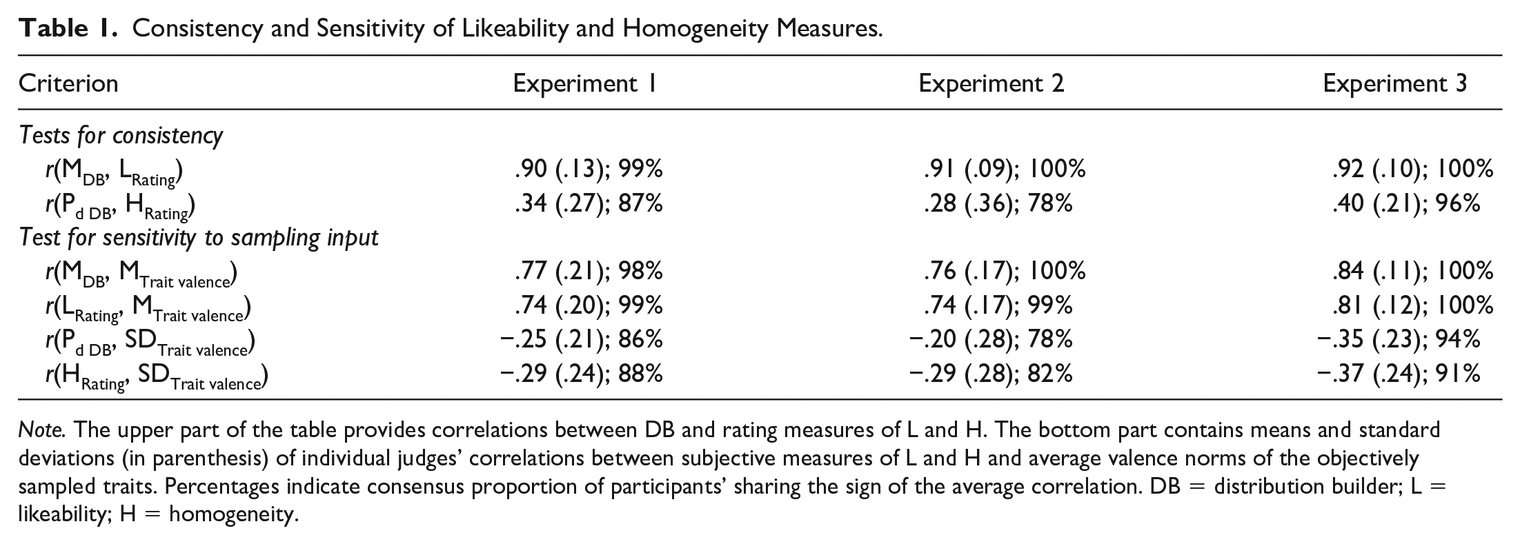
Note. The upper part of the table provides correlations between DB and rating measures of L and H. The bottom part contains means and standard deviations (in parenthesis) of individual judges’ correlations between subjective measures of L and H and average valence norms of the objectively sampled traits. Percentages indicate consensus proportion of participants’ sharing the sign of the average correlation. DB = distribution builder; L = likeability; H = homogeneity.

For an index of sensitivity to sampled input traits, we correlated ratings and distribution builder scores with the average valence norms of the sampled traits.⁶ The correlations in the bottom of Table 1 corroborate that judgments were highly sensitive to the valence norms of the sampled traits. Likeability measures correlated strongly with average valence scale values of the sampled traits (r ranging from .76 to .84 across experiments). Consensus rates across participants were close to 100% (see Table 1).

An analogous homogeneity measure was calculated from the distribution builder. We applied Linville et al.’s (1989) probability of differentiation⁷ P_d. Both measures of homogeneity converged moderately: The distribution-builder P_d correlated with homogeneity ratings in the range of r = .28 to .40 (across experiments). Parallel to merging distribution builder and rating scale values for judgment strength J, we also generated merged homogeneity values H by averaging z-standardized homogeneity ratings and distribution builder P_d values. Both homogeneity measures correlated moderately with samples’ valence norm standard deviations (i.e., inverse homogeneity; average r between −.20 and −.37). To improve reliability, we used merged values from rating scales and distribution builder of J and H for all following hypothesis tests.

Valence and Extremity as Antecedents of Truncation Effects

The four population sets from which samples were drawn allowed for an orthogonal test of the impact of two valence measures of diagnosticity. When predicting $\sqrt{n},$ H, and J from the proportion p of positive traits in the population sets (p = .20, .33, .67, .80), the influence of negative versus positive valence should be manifested in a linear trend (from .20 to .80) whereas the influence of extreme (.20, .80) versus moderate valence (.33, .67) should be evident in a quadratic trend.

Consistent with the expectation that more diagnostic traits facilitate earlier truncation, regression analyses of $\sqrt{n}$ showed that (the square root of) sample size tended to be smaller for negative (linear β: M = .26, SD = 1.15) and for extreme population sets (quadratic β: M = −.24, SD = 1.13) than for positive and moderate population sets.

Likewise, the analysis of judgment strength confirmed the expectation of a diagnosticity effect on judgment polarization. Negative and extreme sets evoked stronger impressions than positive and moderate ones (linear β: M = −1.02, SD = 1.08; quadratic β: M = .83, SD = 1.05). Recall that impression strength J is a deviation score with a positive sign when likeability L deviates from the scale midpoints in the correct direction and reversed L otherwise. In the analysis of homogeneity judgments H, groups described by negative and extreme compared with positive and moderate population sets appeared more homogeneous (linear β: M = −.52, SD = 1.08; quadratic β: M = .62, SD = 1.06; see Table 2).

Table 2.

Means (Standard Deviations) of Individually Calculated ß Weights Obtained in Experiment 1 When Regressing $\sqrt{n}$ , H, and J on the Linear and Quadratic Trend of Population Set Valence p.

Criterion	p (linear): Positivity	p (quadratic): Extremity
Sample size $\sqrt{n}$	β = .26 (1.15)	β = −.24 (1.13)
	t(118) = 2.50, p = .014	t(118) = 2.28, p = .024
	62%	62%
Homogeneity H	β = −.52 (1.08)	β = .62 (1.06)
	t(118) = 5.29, p < .001	t(118) = 6.34, p < .001
	67%	71%
Impression strength J	β = −1.02 (1.08)	β = .83 (1.05)
	t(118) = 10.30, p < .001	t(118) = 8.63, p < .001
	82%	80%

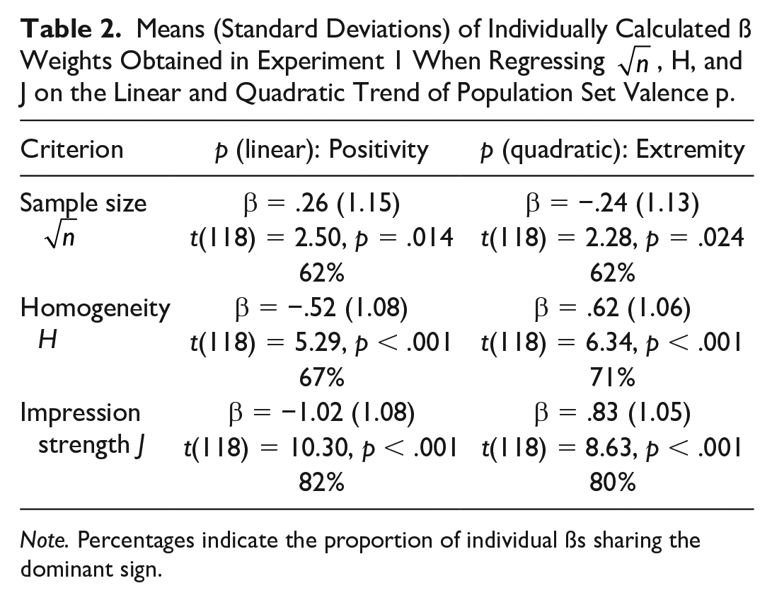
Note. Percentages indicate the proportion of individual ßs sharing the dominant sign.

Truncation Effects on H and J

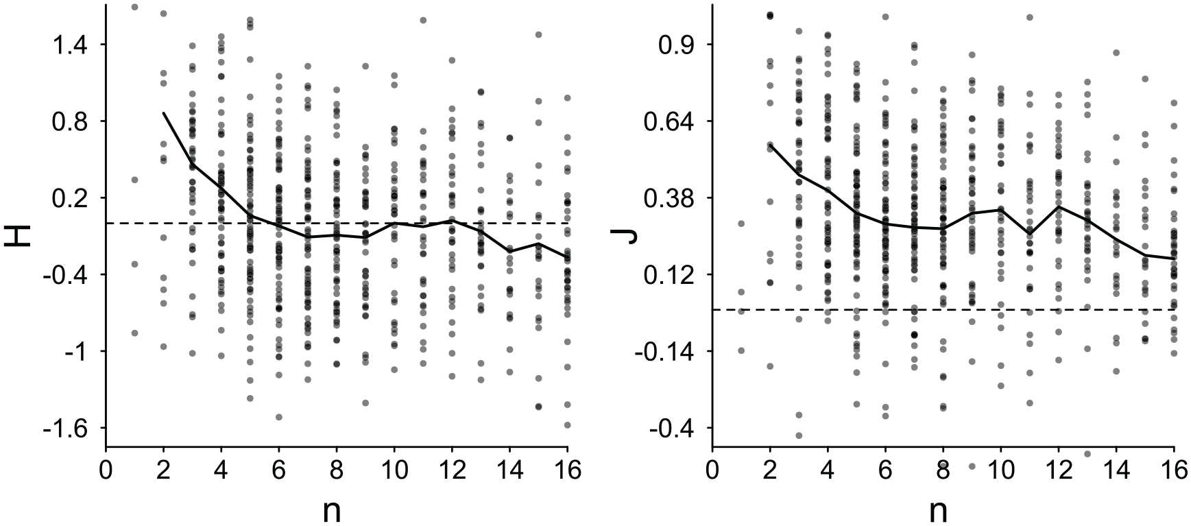
How would truncation and the resulting variation in sample size affect group judgments? Within each individual participant we calculated the correlations across trials of sample size $\sqrt{n}$ with impression strength J and with homogeneity H, after we had averaged over z-standardized measures (distribution builder outcomes and ratings) of J and H. The scatter diagrams in Figure 5 reflect typical self-truncated patterns. Table 3 (left column) gives the corresponding mean sample sizes (and standard deviations) of sample size n, homogeneity scores H, impression strength scores J, and the average individual correlations r_√n,J, r_√n,H, and r_J,H, (across 28 judgments).

Figure 5

Perceived Homogeneity H (left) and Impression Strength J (right) Plotted as Function of Self-Truncated Sample Size n.

Table 3.

Means (Standard Deviations) and Consensus Percentage by Experimental Conditions.

Variable	Pooled for both conditions	Meaningful social group labels	Meaningless labels
n	7.68 (3.74)	7.69 (3.90)	7.67 (3.60)
H	0 (.740)	−.04 (.38)	.05 (.43)
J	.28 (.11)	.25 (.12)	.32 (.09)
$r_{\sqrt{n}, H}$	−.20 (.25); 74%	−.18 (.26); 68%	−.22 (.25); 81%
$r_{\sqrt{n}, J}$	−.19 (.23); 82%	−.15 (.24); 77%	−.23 (.21); 88%
$r_{H, J}$	.42 (.24); 93%	.40 (.26); 90%	.45 (.23); 96%

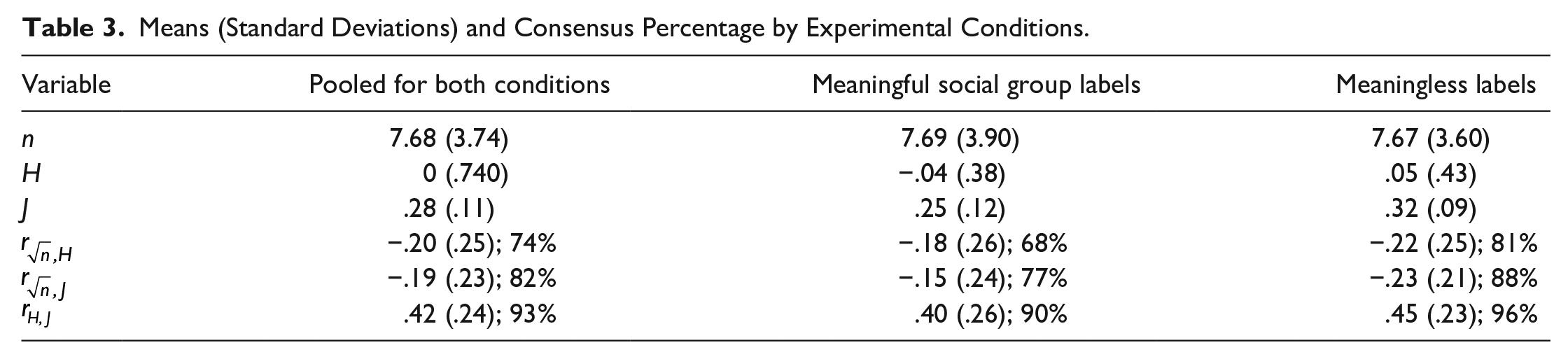
Several sensible findings deserve to be emphasized. First, a strong overall tendency toward positive J scores shows that participants were highly sensitive to actually existing trends in the population sets from which trait samples were drawn. Yet, there was sufficient variation across trials in $\sqrt{n}$ , J, and H to allow for marked correlations, as evident from the first column of Table 3. Impression strength J and homogeneity H correlated strongly and positively over trials. Most importantly, self-truncation effects on J and H manifested in clearly negative correlations, $r_{\sqrt{n}, J}$ and $r_{\sqrt{n}, H}$ between sample size and inter-group bias, generalizing across a large majority of participants: mean $r_{\sqrt{n}, H} =$ −.20, SD = .25 (consensus in sign: 74%); mean $r_{\sqrt{n}, J} =$ −.19, SD = .22 (consensus 82%).

Knowledge: Effects of Meaningful Group Labels

A comparison of the second and third column of Table 3 shows that the group-label manipulation hardly affected the results. Whether traits referred to naturally existing groups with a familiar name or to samples with arbitrary ad hoc labels, the same fundamental self-truncation effects emerged. A small n in a sample carrying a meaningless label yielded virtually the same inferences of group homogeneity and impression strength as impoverished knowledge about an existing minority out-group. Comparing $r_{\sqrt{n}, H}$ , t(117) = .90, d=.17, p=.367, and $r_{\sqrt{n}, J}$ , t(117) = 1.84, d=.34, p=.069, between conditions yielded no noticeable difference. Table 3 also reveals that group labels had no influence on sample size n, t(117) = .04, d = .01, p = .968, and on H, t(117) = 1.22, d = .22, p = .227. The only significant impact of group labels referred to J; knowledge associated with meaningful group labels apparently provided a remedy to strong polarization, evoking weaker judgments on meaningfully labeled groups, t(117) = 3.64, d = .67, p < .001.

Discussion

Regular and consistent results corroborate the reliability of various measures of group impression judgments obtained in Experiment 1, testifying to participants’ motivation and commitment. The average pretest valence scores (i.e., valence of trait population sets from which the samples were drawn) afforded a powerful predictor of group judgments, reflecting the sampled contents. The results obtained with the “distribution builder” (Sharpe et al., 2000) strongly converged with rating measures of group impression judgments, suggesting that the distribution builder offers a valuable instrument for group judgment research.

Experiment 1 suggested that the same functional rules that describe impression judgments of individuals from trait samples (Prager et al., 2018) also apply to samples describing groups. We consolidated the truncation effects obtained for individual impression judgments. The newly added homogeneity measures broadened the perspective and allowed to also assess homogeneity effects. Impressions were stronger and more homogeneous for smaller than for larger samples, analogous to the well-known polarization and homogenization of (small) out-group samples (Brewer, 1993; Linville & Jones, 1980; Quattrone & Jones, 1980).

Comparisons of judgments of existing groups with meaningful labels to mere trait samples of unknown groups with meaningless labels did not reflect a systematic influence of prior knowledge. Sample truncation effects on homogeneity and polarization were about equally strong in both experimental conditions. The only group-label effect was evident in more cautious likeability judgments for meaningful than for neural labels. The reported evidence corroborates two valence-related determinants of diagnosticity: population set valence and extremity. Despite the reduced entitativity of groups compared with individuals, which might dilute systematic influences on sample truncation and impressions, group judgments showed the same typical tendency as individual judgments toward earlier truncation and stronger judgments when negative and extreme traits rendered information more diagnostic than positive and moderate traits. Consistent with our theorizing, high diagnosticity of sampled traits enhanced the impact of sample size and truncation effects.

Experiment 2

So far, Experiment 1 and 2 pre-studies provided convergent evidence for both antecedent and consequent conditions of self-truncation. As negative and extreme traits are more diagnostic than positive and moderate traits, they predict early truncation at small sample size, n, which in turn predicts high homogeneity H and high impression strength J. Yet, the question remains how the co-occurrence of the two major phenomena of inter-group judgments, out-group homogeneity and out-group polarization, can be explained. One plausible answer is that H and J may not be independent. The variance of extreme population sets (at p = .2 and p = .8) may be more restricted than the variance of moderate population sets (at p = .33 and p = .67), the coincidence of J and H may be an artificial consequence of the ecological populations from which traits are sampled.

To disentangle perceived homogeneity from the variability of traits in the population sets conceived as an antecedent condition, in Experiment 2, we deliberately manipulated population set variability orthogonally to valence of the population sets. At each valence level p, we constructed two parallel trait sets, one with traits of high variability in their valence values and one with traits of low variability. If the perceived homogeneity continues to be higher for small than for large groups in such an orthogonal design, this can no longer reflect the restricted variance of extreme population sets. Our theoretical approach implies a persistent influence of diagnosticity (valence × extremity) even when trait variability is controlled for.

Method

Participants and Design

Ninety-four participants were recruited for the second experiment via the Psychology subject pool at Heidelberg University. The experiment was conducted as an online study, which was controlled by PHP and JavaScript. Participants’ age was 18 to 59 years (23.56 years on average), of which 72 identified themselves as female, 20 as male and 2 as other. Eighty-seven students (22 psychology students) participated. We excluded 11 participants’ data from data analysis, because they constantly sampled either n = 1 (minimum) or n = 12 (maximum), leaving data from 83 participants in the analysis.

Materials

Both design factors, the positivity proportion p of traits in different population sets and trait variability, varied within participants, across 20 impression judgment trials. Because trait populations of extreme valence are naturally more homogeneous in valence than moderate ones, we had to fundamentally change the procedure of forming population sets. First, we fixed the population set size to 12 traits to gain more control over the population set characteristics. In an iterative procedure, we then repeatedly sampled n = 12 traits randomly (with replacement) from the total set of 70 traits until the selected sets sufficiently approximated the desired properties. To manipulate valence, we chose five levels of positivity p, namely, 2, 4, 6, 8, and 10 positive out of 12 traits. For each of these five valence levels, we selected parallel population sets, two of (identical) high and two of low within-set variability. We aimed at symmetry in valence mean, approximate equivalence in density and word frequency. The iterative procedure made sure (by repeated sub-sampling from the potential n=12 population set) that not only the entire set, but also sub-set statistics of each population set remained stable with regard to the parallel variability levels, valence, and control measures. By generating two sets per parameter combination (i.e., 5 p-levels × 2 variability levels), 20 population sets were formed in total. A side benefit resulted from this procedure: Valence now had a slightly higher resolution and precision than before; the 20 population sets now covered five instead of four steps of negative versus positive valence (i.e., p varying from 2/12 to 10/12).

Procedure

The remaining procedure was identical to Experiment 1. Each participant provided judgments of 20 self-truncated trait samples representing all 20 population sets, with meaningless group labels. Set order within the experiment and the order of traits within each set were randomized for every participant.

Results

Valence and Extremity as Antecedents of Truncation and Direct Sampling Effects

To replicate the basic results from Experiment 1, we ran regression analyses treating $\sqrt{n}$ (truncation) and H and J as criteria and p (valence and extremity represented by the linear and quadratic trend of p) as diagnosicity predictors, in addition to the within-set variability factor. Note that all three predictors, valence (linear p), extremity (quadratic p), and trait variability, are orthogonal by design, making interaction terms obsolete.

Table 4 and Figure 6 summarize the regression results, which replicate and consolidate the findings of Experiment 1. Samples were truncated earlier, leading to stronger (J) and more homogeneous (H) group judgments, when traits were sampled from more negative and more extreme the population sets . Consequently, samples from negative and extreme sets, compared with positive and moderate sets are judged more strongly (J) and more homogeneous (H).

Table 4.

Means (Standard Deviations) of Individually Calculated Standardized ß Weights Obtained in Experiment 2 When Regressing $\sqrt{n}$ , H, and J on the Linear and Quadratic Trend of Population Set Valence p.

Criterion	Predictors
Criterion	p (linear): Positivity	p (quadratic): Extremity	Variability
Sample size $\sqrt{n}$	β = .44 (1.23)	β = −.37 (1.21)	β = .03 (.20)
	t(82) = 3.24, p = .002	t(82) = 2.79, p = .007	t(82) = 1.53, p = .131
	60%	61%	58%
Perceived homogeneity H	β = −.57 (1.20)	β = .68 (1.12)	β = .10 (.25)
	t(82) = 4.37, p < .001	t(82) = 5.50, p < .001	t(82) = 3.66, p < .001
	70%	71%	66%
Impression strength J	β = −1.90 (1.03)	β = 1.79 (1.00)	β = .06 (.20)
	t(82) = 16.86, p < .001	t(82) = 16.24, p < .001	t(82) = 2.89, p = .005
	96%	98%	66%

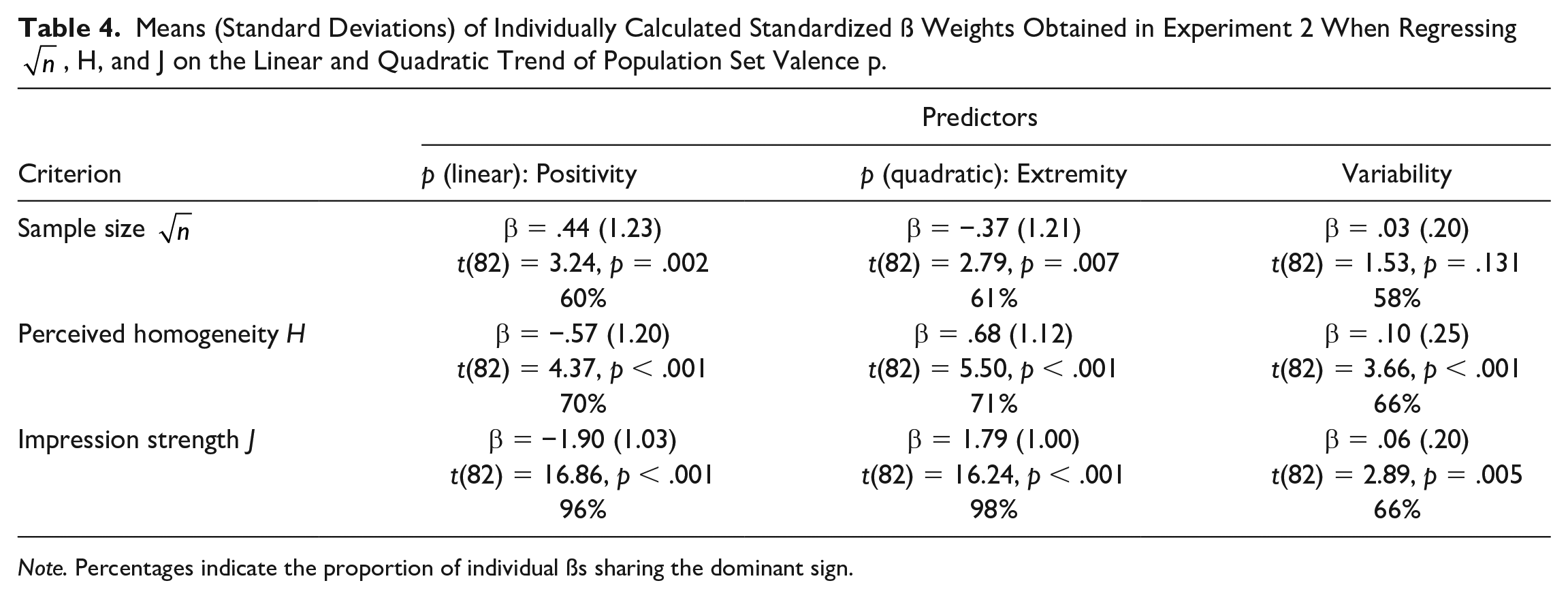
Note. Percentages indicate the proportion of individual ßs sharing the dominant sign.

Figure 6

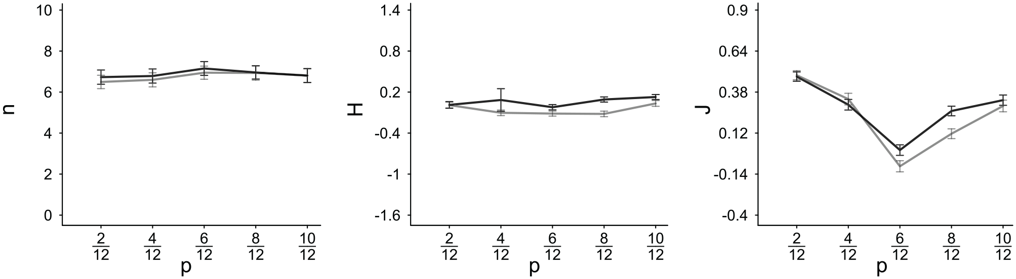
Sample Size, Homogeneity H, and Impression Strength J, Plotted as a Function of Population Set Proportion of Positive Traits p (on the Abscissa).

Within-Set Variability

The design factor, within-set variability at different p levels, hardly explained any variance in $\sqrt{n}$ and J, beyond valence and extremity. Not surprisingly, variability did receive a significant regression weight when predicting homogeneity H, as indicated by the divergence of the light and dark curves in the left bottom chart of Figure 6. Nevertheless, valence and extremity together accounted for more variance in perceived homogeneity than population set variability.

Experiment 3

Experiment 3 aims at directly testing the density account of self-truncation in group impression judgments. If the average distance of traits to all other traits is the crucial stimulus property that drives the impact of sampling and truncation on group judgments, the distance norms should explain for a substantial part of variance in regression analyses of $\sqrt{n}$ , H, and J, beyond the valence and extremity predictors. It might be worthwhile to emphasize that we deliberately manipulated within-group density. As explained in the introduction, perceived stability, and convergence—in other words high within-group density—should facilitate early truncation, and result in strong judgments. Conversely, negative and extreme groups stand out from other groups or perhaps the expectations on groups in general, reflecting low between-group density. Accordingly, in Experiment 3 we replaced the manipulation of population set variability by a manipulation of average trait density within population sets. This factor was again orthogonal to the valence and extremity manipulation of the p proportions.

Method

Participants and Design

Ninety-eight participants were recruited via the Psychology subject pool at Heidelberg University. The experiment was the second in a series of three unrelated studies (on tradeoff-decisions in an information-purchasing paradigm, and on environmentally sustainable behavior) conducted in the same Psychology lab session at Heidelberg University. Participants were between 17 and 77 years old (M = 26.11), 75 were female. Ninety students (14 Psychology) participated. Four participants, who consistently truncated sampling after one item or did never truncate before automatic stopping (at n = 16) were excluded from the analyses; 94 data sets were analyzed. Both design factors, the positivity proportions p and the trait distance norms at each level of p, varied within participants, across 34 trials.

Materials

As in Experiment 2, the aim was to generate population sets of orthogonal within-set distance, valence (linear p), and extremity (quadratic p). As positive (negative) valence and high (low) density are naturally related in the ecology (see Unkelbach et al., 2008), we relied on a similar iterative procedure as in Experiment 2 to accomplish an orthogonal manipulation. Setting the maximum observable sample size to 16, we defined 17 p levels, ranging from 0 up to 16 positive traits (out of 16). For each of these 17 valence levels, we formed two parallel population sets: one of high and one of low average within-set density (resulting in the aforementioned 34 trials). The population sets were formed by an iterative sampling algorithm, where possible population sets were repeatedly drawn (with replacement) from all available traits. As in Experiment 2, potential sets were re-sampled by the iterative procedure when they did not suffice the required characteristics.

Procedure

Each participant engaged in self-truncated sampling and judgments on 34 unlabeled groups corresponding to the 34 population sets. Set order within the experiment and the order of sampled traits within the sets were randomized for every participant.

Results

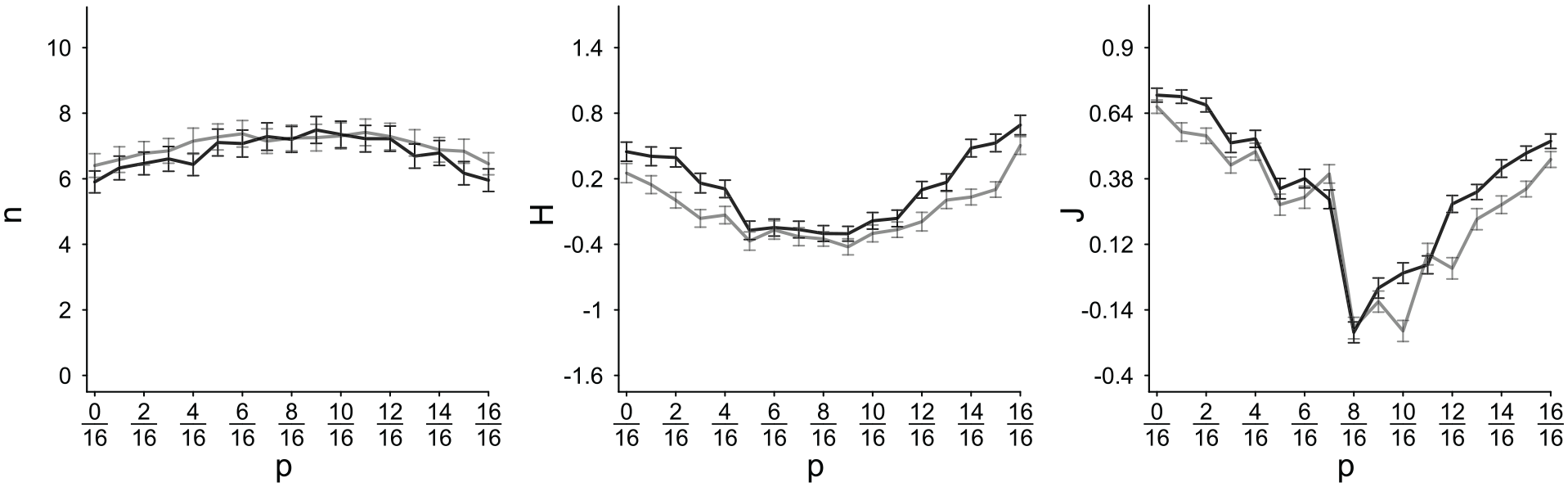
Again, valence and extremity strongly predicted all three criteria $\sqrt{n}$ , H, and J in a series of regression analyses, replicating the same robust pattern as in previous experiments. However, including the average distance score of sampled traits as a third predictor, along with the linear (valence) and quadratic (extremity) p-contrast, created a marked increment in predictive validity. As portrayed in Figure 7 and in the descriptive statistics in Table 5, truncation (small $\sqrt{n}$ ) as well as group impressions (H and J) were not only strongly related to valence and extremity but also to the distance predictor.

Figure 7

Sample Size, Homogeneity H, Impression Strength J, Plotted as a Function of Population Set Proportion of Positive Traits p (on the Abscissa).

Table 5

Means (Standard Deviations) of Individually Calculated ß Weights Obtained in Experiment 2 When Regressing $\sqrt{n}$ , H, and J on the Linear and Quadratic Trend, Density of Population Sets.

Criterion	Predictors
Criterion	p (linear): Positivity	p (quadratic): Extremity	Within-set density
Sample size $\sqrt{n}$	β = .82 (.80)	β = −.79 (.80)	β = −.07 (.18)
	t(92) = 9.93, p <.001	t(92) = 9.56, p < .001	t(92) = 3.54, p = .001
	82%	84%	66%
Homogeneity H	β = −1.23 (.85)	β = 1.35 (.81)	β = .13 (.17)
	t(92) = 14.00, p < .001	t(92) = 16.20, p < .001	t(92) = 7.40, p < .001
	87%	95%	78%
Impression strength J	β = −1.94 (.52)	β = 1.74 (.51)	β = .10 (.13)
Impression strength J	t(92) = 36.29, p < .001	t(92) = 33.03, p < .001	t(92) = 7.33, p < .001
	100%	99%	80%

Note. Percentages indicate how many individual ßs share the dominant sign.

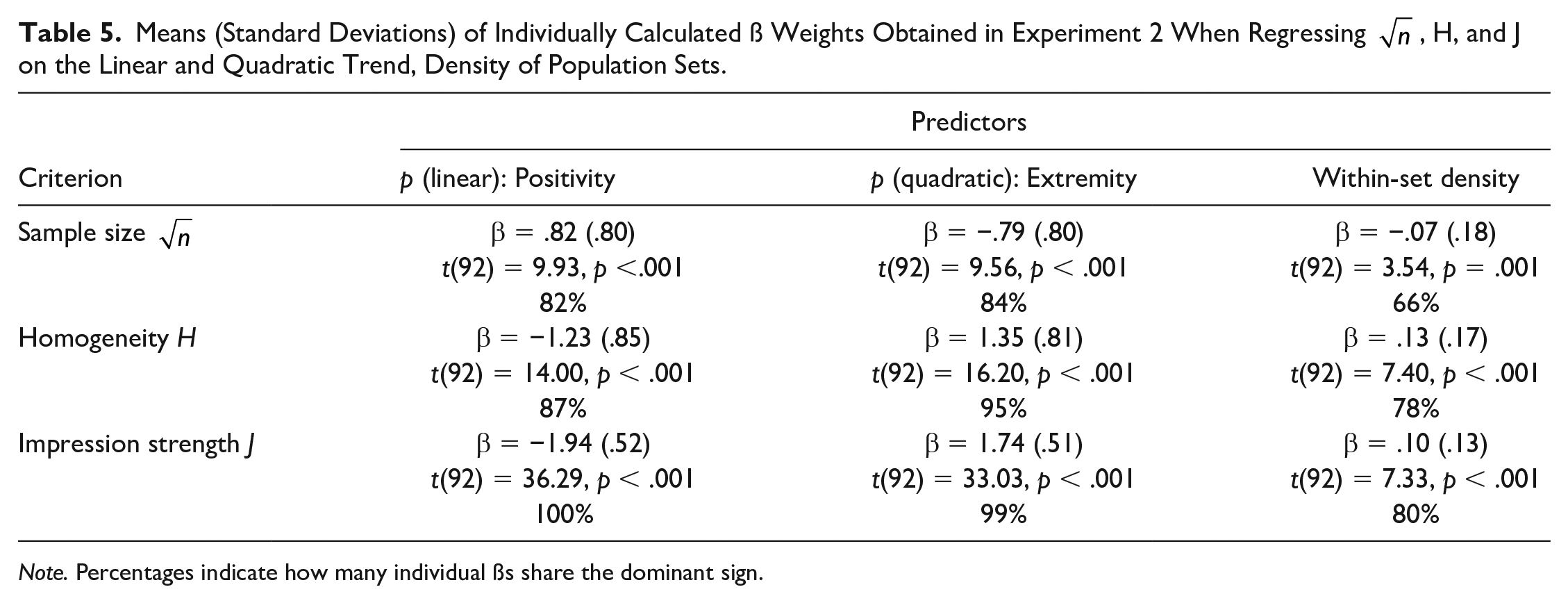
Low within-sample distance (i.e., high density) led to earlier truncation (i.e., smaller n) than high within-sample distance (low density), as evident from a mean regression weight of β = −.07 (.18), t(92) = 3.54, p = .001 and a consensus rate of 66%. Because group judgments were not only affected indirectly by the truncation effect but also directly reflected the properties of sampled traits (see Figure 7), distance received a stronger regression weight in predictions of H, mean β = .13 (SD=.17), t(92) = 7.40, p < .001, 78% consensus, and J, β = .10 (SD=.13), t(92) = 7.33, p < .001, 80% consensus. Both perceived homogeneity (H) and impression polarization increased with decreasing trait distance.

Thus, consistent with the density-model hypothesis, average trait distance within samples contributed to the prediction of early truncation (small n) and group judgments of J and H. Recall that this contribution reflects the diagnosticity of traits beyond variability of traits in the population set.

General Discussion

In sum, all simulation results and empirical findings obtained in the present research converge to a robust but nevertheless refined pattern that allows us to draw distinct conclusions. Our research highlights that sample-based impression judgments follow the same set of sampling rules regardless of whether the sampled traits characterize an individual target or whether each trait refers to a different member of a social group. In either case, impression judgments are highly sensitive not only to the parameters of the population sets from which samples are drawn, but also to the diagnosticity of the sampled traits, as determined in careful pilot testing.

Notably, the resulting impression judgments systematically deviated from a simple averaging rule (Anderson, 1965). Trait diagnosticity strongly moderated the impact of a newly added trait on the sequential impression updating process. We were able to isolate distinct diagnosticity aspects; in addition to negative (vs. positive) valence and extremity, a trait’s high average distance to the other traits within the sample (according to the density-model framework) provided a third source of diagnosticity. The research design of all experiments involved pre-selected population sets from which samples were drawn randomly.

Although the entire pattern corroborates the usefulness and fertility of our sampling-theoretical approach to impression formation, the main original contribution of our research consisted in the delineation of self-truncation effects, thereby offering a completely novel perspective on inter-group judgment. The law of large numbers and Bayesian updating of flat priors predict that the same proportion (e.g., proportion of positive traits, correct student responses, or favorable consumer ratings) provides stronger evidence when observed in a larger than in a smaller sample (Bernoulli, 1713; Tversky & Kahneman, 1971). Thus, 12 positive votes in a sample of n = 16 provide stronger evidence for a positive outcome rate of 75% than the same proportion of three positive outcomes in n = 4, as long as sample size is treated as independent variable. However, self-truncation causes a notable reversal of the positive relation between evidence strength and sample size. When the first few observations happen to reflect a strong and regular trend (e.g., three or four positive outcomes in n = 4), early truncation produces polarized and homogeneous samples that can be expected to trigger strong and conflict-free judgments. In the absence of such a stochastic primacy effect, samples of increasing size are quite unlikely to reach similarly extreme proportions and reduced variance as is possible in early phases of growing samples. Thus, because self-truncated samples can be expected to remain small if they exhibit strong and conflict-free patterns but become large when the initial evidence is weak and conflict-prone, it is no surprise that self-truncated samples tend to convey stronger evidence when they are small rather than large.

Note that this strong reversal from a positive correlation between sample size and evidence strength with experimenter-determined n to a negative correlation with self-truncated n is possible because n is no longer an independent variable but dependent on the judge’s primacy impression of the strong evidence that justifies early truncation. Conversely, a large self-truncated n is reflective of judge’s appraisal that the sample started with weak evidence that did not justify earlier truncation.

Two important implications of self-truncation effects deserve to be emphasized. First, although the evidence for a strong reversal from a positive to a negative impact of sample size on evidence strength has been found in previous experiments and substantiated in simulation studies (Fiedler et al., 1999; Fiedler et al., 2010; Prager & Fiedler, 2021), its relevance for political, economic, or health-related judgments and decisions is hardly recognized. For instance, protocols of democratic decision groups do not reveal whether a discussion underlying a consequential decision was self-truncated or externally determined, whether a job candidate was interviewed for a fixed timeframe or whether the interviewers deliberately terminated the dialogue at some point, or whether consumer choices were informed by self-truncated or externally truncated search for information. In all these domains, we continue to presuppose that more extensive information acquisition and more careful advice-taking produce more accurate decisions, if only to justify information costs.

Second, it is obvious that sample truncation decisions (i.e., decisions to stop a sequentially unfolding sample) are similarly sensitive to stimulus diagnosticity as the final judgments. The evidence from the present investigation provides strong support for this notion. The enhanced diagnosticity of negative, extreme, and low within-sample-distance traits (compared with less diagnostic positive, moderate, and high-distance traits) not only led to stronger and more homogeneous final impression judgments (manifested in stronger impression strength J and homogeneity H scores) but also enabled earlier truncation, leading to exaggerated sample estimates. As a consequence, the dominant impact of trait diagnosticity on truncation served to amplify the diagnosticity effect on the resulting impressions, as manifested in regularly negative correlations between sample size and impression strength $r_{\sqrt{n}, J}$ and between sample size and homogeneity $r_{\sqrt{n}, H}$ . In addition, we found highly consistent empirical support for the impact of diagnostic trait properties (negativity, extremity, and distance) on judgment strength (J) and homogeneity (H).

Granting that experienced samples are typically smaller for out-groups than for in-groups, the reported findings afford a sufficient account of two major phenomena of inter-group research, out-group homogeneity (H) and out-group polarization (J). Because negative behavior (Reeder & Brewer, 1979) is more diagnostic than positive behavior, enhanced homogeneity and polarization implies out-group derogation. Consistent with this sample size account of inter-group biases, pertinent research has shown that out-group polarization and homogeneity are ameliorated or even reversed when sample size is larger for out-groups than for in-groups; Simon & Brown, 1987) or when asymmetric social contact serves to reduce the sample-size difference between in-groups and out-groups (Wagner et al., 2006).

For the sake of theoretical clarity, it seems appropriate to emphasize that we do not state that inter-group judgments can be reduced to variation in sample size and diagnosticity. We demonstrated that self-truncated sampling together with differential diagnosticity impacts construes a sufficient, not a necessary condition of inter-group biases. Self-evidently, inter-group bias can as well result from many different causal factors, including real conflicts, resentments, cultural and linguistic influences, closeness of social inter-connections, and the distribution of resources. Rather than propagating one necessary condition supposed to underlie all inter-group biases, we argue, and have provided cogent evidence to demonstrate, that unequal samples size constitutes a sufficient (and parsimonious) condition for the most prominent biases reported in inter-group literature. We believe that this demonstration is very useful for progress in future research, which should try to disentangle inter-group effects that go beyond the basic sampling effects that were the focus of the present article.

Supplemental Material

sj-txt-1-psp-10.1177_01461672231223335 – Supplemental material for Small Sample Size and Group Homogeneity: A Crucial Ingredient to Inter-Group Bias

Supplemental material, sj-txt-1-psp-10.1177_01461672231223335 for Small Sample Size and Group Homogeneity: A Crucial Ingredient to Inter-Group Bias by Johannes Ziegler and Klaus Fiedler in Personality and Social Psychology Bulletin

Footnotes

Appendix

Acknowledgements

Helpful comments by Gaël Le Mens and Linda McCaughey on a draft of this article are gratefully acknowledged.

Declaration of Conflicting Interests

The author(s) declared no potential conflicts of interest with respect to the research, authorship, and/or publication of this article.

Funding

The author(s) disclosed receipt of the following financial support for the research, authorship, and/or publication of this article: The work underlying the present article was supported by a grant provided by the Deutsche Forschungsgemeinschaft (Fi 294/29-1) to the second author.

ORCID iD

Johannes Ziegler

Supplemental Material

Supplemental material is available online with this article. Data and code of the reported studies can be accessed at .

Notes

References

Anderson

N. H.

(1965). Averaging versus adding as a stimulus-combination rule in impression formation. Journal of Experimental Psychology, 70(4), 394–400. https://doi.org/10.1037/h0022280

Bergh

Lindskog

(2019). The group-motivated sampler. Journal of Experimental Psychology: General, 148(5), 845–862. https://doi.org/10.1037/xge0000601

Bernoulli

(1713). Ars conjectandi. [The art of conjecturing]. Thurneysen Brothers.

Brewer

M. B.

(1993). Social identity, distinctiveness, and in-group homogeneity. Social Cognition, 11(1), 150–164. https://doi.org/10.1521/soco.1993.11.1.150

Campbell

D. T.

(1958). Common fate, similarity, and other indices of the status of aggregates of persons as social entities. Behavioral Science, 3, 14–25. https://doi.org/10.1002/bs.3830030103

Denrell

(2005). Why most people disapprove of me: Experience sampling in impression formation. Psychological Review, 112(4), 951–978. https://doi.org/10.1037/0033-295X.112.4.951

Denrell

Le Mens

(2007). Interdependent sampling and social influence. Psychological Review, 114(2), 398–422. https://doi.org/10.1037/0033-295X.114.2.398

Fazio

R. H.

Eiser

J. R.

Shook

N. J.

(2004). Attitude formation through exploration: Valence asymmetries. Journal of Personality and Social Psychology, 87(3), 293–311. https://doi.org/10.1037/0022-3514.87.3.293

Fiedler

(2000). Beware of samples! A cognitive-ecological sampling approach to judgment biases. Psychological Review, 107(4), 659–676.

10.

Fiedler

Kemmelmeier

Freytag

(1999). Explaining asymmetric inter-group judgments through differential aggregation: Computer simulations and some new evidence. European Review of Social Psychology, 10(1), 1–40.

11.

Fiedler

Renn

S.-Y.

Kareev

(2010). Mood and judgments based on sequential sampling. Journal of Behavioral Decision Making, 23(5), 483–495. https://doi.org/10.1002/bdm.669

12.

Fiedler

Wänke

(2009). The cognitive-ecological approach to rationality in social psychology. Social Cognition, 27(5), 699–732. https://doi.org/10.1521/soco.2009.27.5.699

13.

Fiske

S. T.

(1980). Attention and weight in person perception: The impact of negative and extreme behavior. Journal of Personality and Social Psychology, 38(6), 889–906. https://doi.org/10.1037/0022-3514.38.6.889

14.

Gidron

Koehler

D. J.

Tversky

(1993). Implicit quantification of personality traits. Personality and Social Psychology Bulletin, 19(5), 594–604. https://doi.org/10.1177/0146167293195011

15.

Goldstone

(1994). An efficient method for obtaining similarity data. Behavior Research Methods, Instruments & Computers, 26(4), 381–386. https://doi.org/10.3758/BF03204653

16.

Haldane

J. B. S.

(1945). A labour-saving method of sampling. Nature, 155, 49–50.

17.

Kareev

Arnon

Horwitz-Zeliger

(2002). On the misperception of variability. Journal of Experimental Psychology: General, 131(2), 287–297. https://doi.org/10.1037/0096-3445.131.2.287

18.

Koch

Imhoff

Dotsch

Unkelbach

Alves

(2016). The ABC of stereotypes about groups: Agency/socioeconomic success, conservative–progressive beliefs, and communion. Journal of Personality and Social Psychology, 110(5), 675–709.

19.

Konovalova

Le Mens

(2020). An information sampling explanation for the in-group heterogeneity effect. Psychological Review, 127(1), 47–73. https://doi.org/10.1037/rev0000160

20.

Le Mens

Denrell

. (2011). Rational learning and information sampling: On the “naivety” assumption in sampling explanations of judgment biases. Psychological Review, 118(2), 379–392. https://doi.org/10.1037/a0023010

21.

Linville

P. W.

Fischer

G. W.

(1993). Exemplar and abstraction models of perceived group variability and stereotypicality. Social Cognition, 11(1), 92–125. https://doi.org/10.1521/soco.1993.11.1.92

22.

Linville

P. W.

Fischer

G. W.

Salovey

(1989). Perceived distributions of the characteristics of in-group and out-group members: Empirical evidence and a computer simulation. Journal of Personality and Social Psychology, 57(2), 165–188. https://doi.org/10.1037/0022-3514.57.2.165

23.

Linville

P. W.

Jones

E. E.

(1980). Polarized appraisals of out-group members. Journal of Personality and Social Psychology, 38(5), 689–703. https://doi.org/10.1037/0022-3514.38.5.689

24.

Park

Rothbart

(1982). Perception of out-group homogeneity and levels of social categorization: Memory for the subordinate attributes of in-group and out-group members. Journal of Personality and Social Psychology, 42(6), 1051–1068. https://doi.org/10.1037/0022-3514.42.6.1051

25.

Prager

Fiedler

(2021). Forming impressions from self-truncated samples of traits: Forming impressions from self-truncated samples of traits–interplay of Thurstonian and Brunswikian sampling effects. Journal of Personality and Social Psychology, 121(3), 474–497. https://doi.org/10.1037/pspa0000274

26.

Prager

Krueger

J. I.

Fiedler

(2018). Towards a deeper understanding of impression formation-New insights gained from a cognitive-ecological perspective. Journal of Personality and Social Psychology, 115(3), 379–397. https://doi.org/10.1037/pspa0000123

27.

Quattrone

G. A.

Jones

E. E.

(1980). The perception of variability within in-groups and out-groups: Implications for the law of small numbers. Journal of Personality and Social Psychology, 38(1), 141–152. https://doi.org/10.1037/0022-3514.38.1.141

28.

Reeder

G. D.

Brewer

M. B.

(1979). A schematic model of dispositional attribution in interpersonal perception. Psychological Review, 86(1), 61–79. https://doi.org/10.1037/0033-295X.86.1.61

29.

Rothbart

Park

(1986). On the confirmability and disconfirmability of trait concepts. Journal of Personality and Social Psychology, 50(1), 131–142. https://doi.org/10.1037/0022-3514.50.1.131

30.

Sharpe

W. F.

Goldstein

D. G.

Blythe

P. W.

(2000). The distribution builder: A tool for inferring investor preferences. https://web.stanford.edu/~wfsharpe/art/qpaper/qpaper.pdf

31.

Simon

Brown

(1987). Perceived intragroup homogeneity in minority-majority contexts. Journal of Personality and Social Psychology, 53(4), 703–711.

32.

Skowronski

J. J.

Carlston

D. E.

(1987). Social judgment and social memory: The role of cue diagnosticity in negativity, positivity, and extremity biases. Journal of Personality and Social Psychology, 52(4), 689–699.

33.

Thorndike

E. L.

(1927). The law of effect. The American Journal of Psychology, 39, 212–222. https://doi.org/10.2307/1415413

34.

Tversky

Kahneman

(1971). Belief in the law of small numbers. Psychological Bulletin, 76(2), 105–110. https://doi.org/10.1037/h0031322

35.

Unkelbach

Fiedler

Bayer

Stegmüller

Danner

(2008). Why positive information is processed faster: The density hypothesis. Journal of Personality and Social Psychology, 95(1), 36–49. https://doi.org/10.1037/0022-3514.95.1.36

36.

Wagner

Christ

Pettigrew

T. F.

Stellmacher

Wolf

(2006). Prejudice and minority proportion: Contact instead of threat effects. Social Psychology Quarterly, 69(4), 380–390. https://doi.org/10.1177/019027250606900406

37.

Yzerbyt

Castano

Leyens

J. P.

Paladino

M. P.

(2000). The primacy of the ingroup: The interplay of entitativity and identification. European Review of Social Psychology, 11(1), 257–295.

Supplementary Material

Please find the following supplemental material available below.

For Open Access articles published under a Creative Commons License, all supplemental material carries the same license as the article it is associated with.

For non-Open Access articles published, all supplemental material carries a non-exclusive license, and permission requests for re-use of supplemental material or any part of supplemental material shall be sent directly to the copyright owner as specified in the copyright notice associated with the article.

0.00 MB