
Abstract
Many analytical approaches to single-case data assume either linear effects (regression-based methods) or instant effects (mean-based methods). Neither assumption is realistic; therefore, these approaches’ assumptions are often violated. In this article, we propose modeling curvilinear effects to appropriately parametrize the characteristics of singe-case data. Specifically, we introduce the generalized logistic function as adequate function for this situation. The merits of the proposed procedure are demonstrated using data previously used in single case research that represent typical single case data. We provide the function with auxiliary graphical options to demonstrate the model parameters. The function is freely available in the R package “userfriendlyscience.” The proposed procedure is a new way to analyze single case data, which may provide applied single case researchers with a new tool to better understand their data and avoid applying methods with violated assumptions.
Single case designs (SCDs) are increasingly recognized as important tools in behavior modification research and other fields, enabling researchers to model changes in psychological or behavioral variables over time (Franklin, Allison, & Gorman, 2014). Common approaches to analysis of SCDs are based on comparing means before and after an intervention or modeling the slope of a change using regression-based techniques (Manolov & Moeyaert, 2017a). These techniques have the advantage that they are familiar to many researchers and are readily available in statistical packages. However, the models underlying these most commonly employed analysis techniques have assumptions that are often violated. Specifically, an intervention effect on a psychological construct typically manifests neither as a discontinuous shift from one value to another (the model underlying comparison of means), nor a linear unbounded change over time (the model underlying linear regression). Instead, intervention effects often reflect a shift in a psychological construct where both the initial and the final values are more or less stable over time. Accurate modeling of this shift provides more information about treatment effects than comparison of means or estimating the slope of a change. In this article, we introduce a technique for such modeling as well as freely available user friendly functions implemented in R (R Core Team, 2018). We illustrate this technique through the use of two data sets and provide a brief tutorial to make these techniques widely accessible.
SCDs are important because they provide a means to determine the effectiveness of interventions at an individual level (Barlow, Nock, & Hersen, 2009). Much methodological research has been devoted to effect size measures in SCD because an accurate effect size supports the development of evidence-based interventions (Parker et al., 2005; Parker & Hagan-Burke, 2007; Parker, Vannest, & Davis, 2011). An effect size can be considered accurate if it provides a reliable indication of, for instance, the improvement of a patient after or during treatment. The type of effect size is closely related to what type of analysis of SCDs is chosen (Lenz, 2015; Vannest & Ninci, 2015). Two basic classes of analyses can be distinguished: first parametric regression-based methods, including multilevel analysis (Baek et al., 2014), and second nonparametric methods. A recent overview of analysis techniques for SCD is given by Heyvaert and Onghena (2014).
Comparison of means before and after an intervention represent the most straightforward analysis, but the underlying model holds that a change manifests as an instantaneous shift from one stable value to another, which is often not realistic. In addition, this analysis cannot infer from the data when such a shift may occur: The user must specify which data points to aggregate in each mean. Thus, although this approach’s familiarity may partly explain its prevalence, this analysis’ assumption of instantaneous change from one otherwise stable value to another is rarely realistic, and it yields little information about the treatment.
More advanced regression-based approaches for analyzing SCDs usually (but not necessarily) consider a linear model, and, therefore, can accommodate incremental change, no longer imposing an instantaneous shift of the criterion from one value to another. For example, in a pre–post design, the piecewise regression (PWR) model (Center, Skiba, & Casey, 1985; Huitema & McKean, 2000) can be used to model a linear trend separately for two phases: one before the intervention and one during or after the intervention. This model then compares the intercepts and slopes between both phases of the design, and intervention effects are derived from the differences in slopes and intercepts. Although many more sophisticated PWR models exist, for example, piecewise splines (e.g., Friedman, 1991), these more complex methods remain relatively uncommon, perhaps, ironically, because their sophistication renders them less accessible to many researchers. The commonly used two-phase method suffers from the problem that it assumes that the change manifests in a linear fashion: the slope only changes once and then remains the same. This is unrealistic for two reasons.
First, in many situations, for instance, when the effects of a therapy are monitored, the criterion is measured by some sort of questionnaire or other operationalization that has a limited range. The observed or measured improvement of clients in a therapeutic setting is, therefore, artificially constrained by the scale of the instrument. A 7-point Likert-type scale is an example of such an instrument. If clients rate how they feel with a maximum score of seven, there is no further room for improvement. The score of seven in this example constitutes a ceiling in the therapy effect. Likewise, such an instrument has a floor, which is the minimum value of the scale. A straight line would break through the ceiling (or floor, when the criterion decreases over time), unless the therapy has no effect.
Second, treatments and interventions in the clinical and health psychology practice are often protocolled, and as a consequence, have a natural limit as to their effectiveness. This is the case because they are designed based on knowledge of the behavior, cognitions, or affective associations that are targeted. If implemented properly, they will affect the areas of human psychology for which they were designed, thereby improving the target behavior or condition. However, no psychological theory or combination of theories explain behavior or psychopathology completely. Therefore, evidence- and theory-based interventions and treatments are necessarily limited in terms of the effect they can have: at most, they can have the maximum achievable effect in all areas they target, and they do not target the whole of human psychology. This characteristic manifests as a constraint for treatment effectiveness. For example, an exposure therapy treatment for an anxiety disorder based on inhibitory learning (Craske, Treanor, Conway, Zbozinek, & Vervliet, 2014) cannot be expected to address dysfunctional self-regulation patterns that may have emerged over the course of the anxiety disorder. Theory-based treatment, being based on theory, and theory by definition dealing only with a bounded aspect of reality, necessarily is constrained in its maximum effectiveness. Such a constraint on effectiveness means that the association between time in treatment and treatment effectiveness is unlikely to be linear: change is likely to slow as treatment approaches its maximum possible effect.
Thus, treatment effects realistically manifest as a shift in the targeted construct(s) from a more or less stable level to a new more or less stable level. This shift likely decelerates as the treatment reaches its maximum possible effect. This underlying model is neither accurately captured by comparison of means, nor by a two-phase PWR model. Using more sophisticated spline regression models can address this, but these suffer from two disadvantages. First, they are often not accessible to researchers without more advanced statistical training (which may partly explain the prevalence of the mean comparison and two-phase PWR models despite their relative inadequacy). Second, they are relatively unparsimonious and require estimating a large number of parameters compared with the small number of data points often available in SCD data sets.
In this article, we present a technique that addresses both these points: it is freely available and designed to be easily accessible and usable for a wide variety of researchers and potentially practitioners, and it estimates the same number of parameters as a two-phase PWR model. Specifically, this model is based on an optimization function applied to a generalized logistic model. This enables the estimation of effects in a pre–post SCD design when the criterion is constrained (e.g., has a floor or a ceiling). We will first present an example of the model and show its mathematical characteristics. Then we present two clinical examples in which we compare the proposed model with the PWR model. Finally, we discuss some possibilities for future research.
The Problem With Ceilings
This distribution shown in Figure 1 illustrates a likely model for an intervention process, with the x axis representing time (e.g., in days) and the y axis an outcome (where higher values are more desirable). The first five measurements were taken before the intervention. Although five points are too few to obtain reasonably tight confidence intervals (CIs), this small number is often seen in practice. The values show variability around the fitted line, which is essentially a plateau. Once the intervention commences, however, each session has (on average) some effect to improve the outcome. In this ideal situation, once all targeted areas have been improved, no additional effects can be expected: therefore, after roughly 20 days, the intervention no longer has any effect and another plateau is reached.
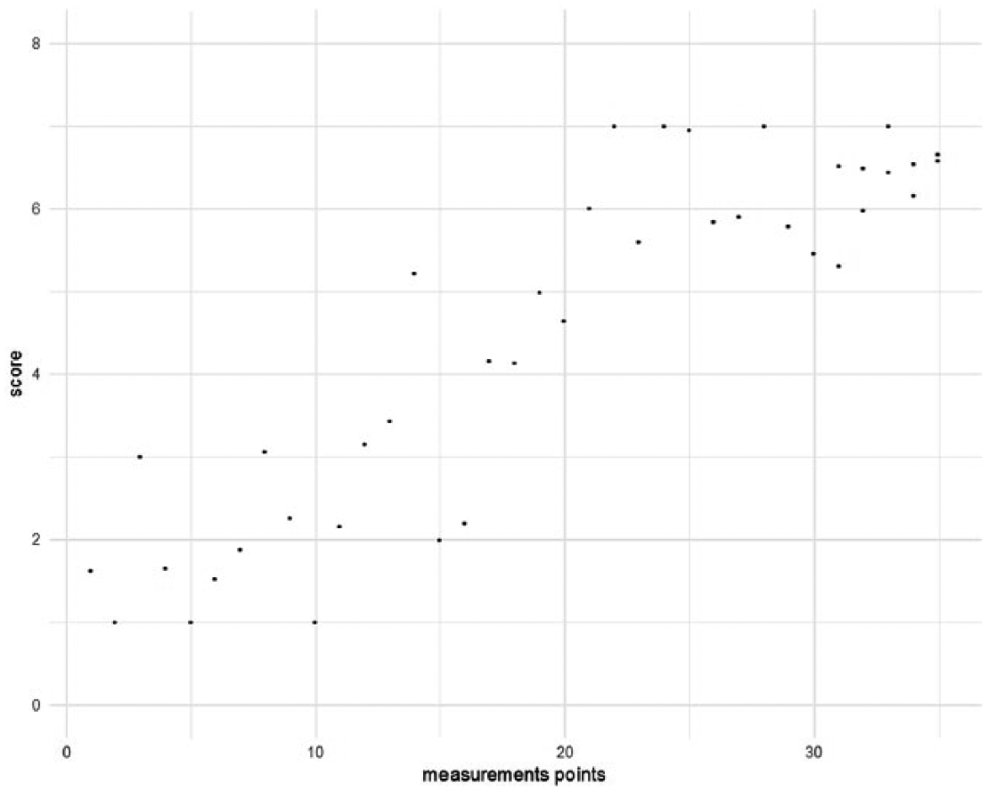
Example with generated data from generalized logistic model for t = 6 to 30 (B = .4, x0 = 10, v = 1).
A simple model assuming a linear relationship seems to predict these data rather well, see Figure 2. The deviance (sum of the squared residuals) of the linear model is Dlm = 34.3, with R2 = .80. This is partly due to the fact that the pre-intervention and stability phases are rather short in this example.
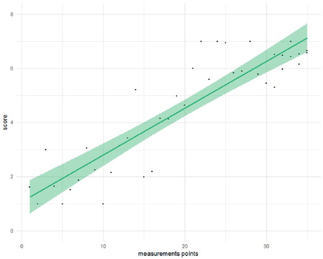
Example with generated data from generalized logistic model with linear fit added (b0 = 1.07; b1 = 0.17; R2 = .80).
However, the residuals from the “straight-line” model seem to show a cyclic or auto-correlated pattern, as Figure 3 clearly shows. One of the assumptions for unbiased parameter in linear regression estimates is homogeneity of the residuals and in this example this assumption is violated. This is an indication that the “straight-line”model is not the correct model to describe these data.
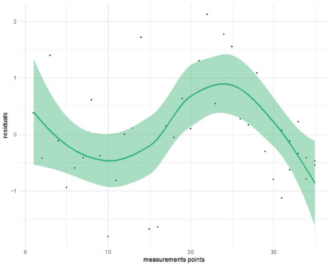
Residuals from linear model of example data.
Despite the high squared multiple correlation, the line misses some important information, in particular the strong increase in scores somewhere between the 15th and 20th point. It is good practice to test the model assumptions. When these assumptions are violated, another model should be fitted to the data.
Consequences for Tests of the Intervention Effect
To test the effect of the intervention, a naive approach is to compare the two means before and after (or during) the intervention. The effect size of the intervention in this approach is Cohen’s (1992) d or simply the difference between the two means divided by the pooled standard deviation (Rosenthal, 1978). In this example d = 1.80, with 95% CI = [0.8, 2.8], a large effect, which corresponds with the visual inspection of the data.
However, claiming an intervention effect because the means in both phases are different is not correct (Huitema & McKean, 2007). When there appears to be a trend in the data (e.g., scores increase over time, independent of the intervention) simply comparing the means of the outcomes in the two phases may lead to wrong conclusions (Center et al., 1985). The trend, instead of an intervention effect, may be responsible for the different means in the two phases. Therefore, it is important to incorporate a trend effect in a research model for SCD data.
To adequately model such trends, a PWR model (Center et al., 1985; Huitema & McKean, 2000) can be used. PWR models two linear trends, separately for both phases. That is, the intercepts and slopes of two regression lines are compared before and after the intervention. See Figure 4 for an illustration. This model is given by

where
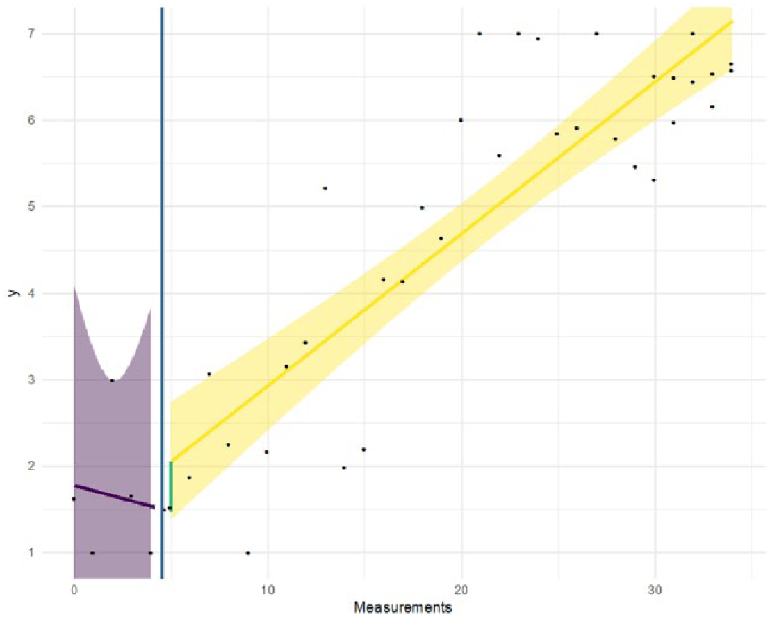
Piecewise regression on example data with trend effect.
In the PWR model, b0 is the score at T = 0 (1.8 in this example), b1 can be interpreted as the change in level between Phase A and B, not confounded with possible trend effects. This effect, 0.58 with 95% CI = [–1.6, 2.7], is represented by the (short) green line; it is the difference between the predicted scores of both regression lines at the first measurement of the second phase. The trend in the baseline Phase A is captured by b2 (–0.06 with 95% CI = [–0.7, 0.6]) and the change in trend from Phase A to Phase B by b3 (0.24 with 95% CI = [–0.4, 0.9]). In this example, the parameter of interest is b3, the change in slope. The postintervention line has a slope of about .18. The very large CIs around b1, b2, and b3 are due to the relatively high heterogeneity when estimating the regression intercept and slope in Phase A, illustrated by the wide purple zone in Figure 4. As there are only five data points, high levels of heterogeneity can be expected. This shows the dangers of having too few baseline points. The deviance of this piecewise model is Dpw = 33.7, which is slightly better than the linear model.
When only a level effect is present in the data, as assumed by the mean comparison approach and shown in another example in Figure 5, the b1 (4.18) parameter would be of primary interest. The change from the slope in the pre-intervention phase (b2 = −0.04) to the flat line in the postintervention phase is as expected 0.05 (b3). Cohen’s d is 7.9 with 95% CI = [5.2, 10.5] in this example (note that in these simulated examples, we generated exaggerated effects to clearly illustrate the patterns in the data).
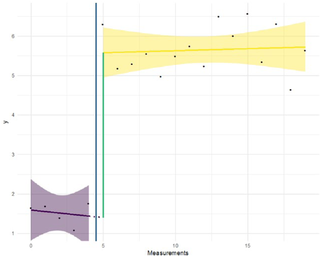
Piecewise regression on example data with instantaneous phase effect.
For this PWR method, the following effect size is defined (Parker & Brossart, 2003):
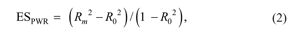
Where
In many situations, it is not only important to know that there exists an effect and how strong it is, but also at what point in time the improvement due to the intervention started, how fast the change occurred, and when the improvement stabilized. For such questions, it is better to fit a curve to the data, which has the form of a sigmoid function, because it reflects the empirical process more accurately and allows for more flexibility.
The Generalized Logistic Model
A sigmoid function can be defined in many ways. Here we choose the generalized logistic (GL) function, which is defined as follows:
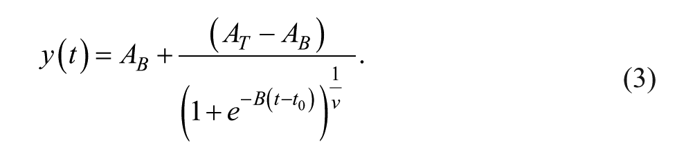
This model has the advantage that it is parametrized relatively straightforwardly: the analysis estimates the initial plateau and the postintervention plateau as well as when the change starts and stops. Specifically, the variable y(t) is the outcome at moment t (where t is either a valid time measurement, for example, in seconds or days since the first measurement, or a rank, such as t = 1, . . ., n). The parameters AB and AT are the asymptotes that indicate, respectively, the minimum (floor) and maximum (ceiling) of the curve. The parameter B is the growth rate, indicating how steep the curve is. The parameter v indicates near which asymptote the maximum growth occurs and t0 (the inflection point) corresponds to the time point at which the curve is at its midpoint (when v = 1). For the parameter values: AB = 0, AT = 1, B = 1, v = 1, and t0 = 0, this function simplifies to the well-known logistic function.
The generalized logistic function was fitted on the example data (Figure 6) with the R function nlsLM() from the package minpack.lm (Elzhov, Mullen, Spiess, & Bolker, 2016). The resulting curve fitted the data well: R2 = .85 and the deviance Dgl = 26.3, which indicates a better fit to the data compared with the simple linear regression and PWR models. The parameters obtained from this analysis were t0 = 17.0, B = 0.20, AB = 1.2, AT = 7.0 (and v was fixed to 1). From this analysis, we learn that the process starts at 1.2 and ends at 7.0.
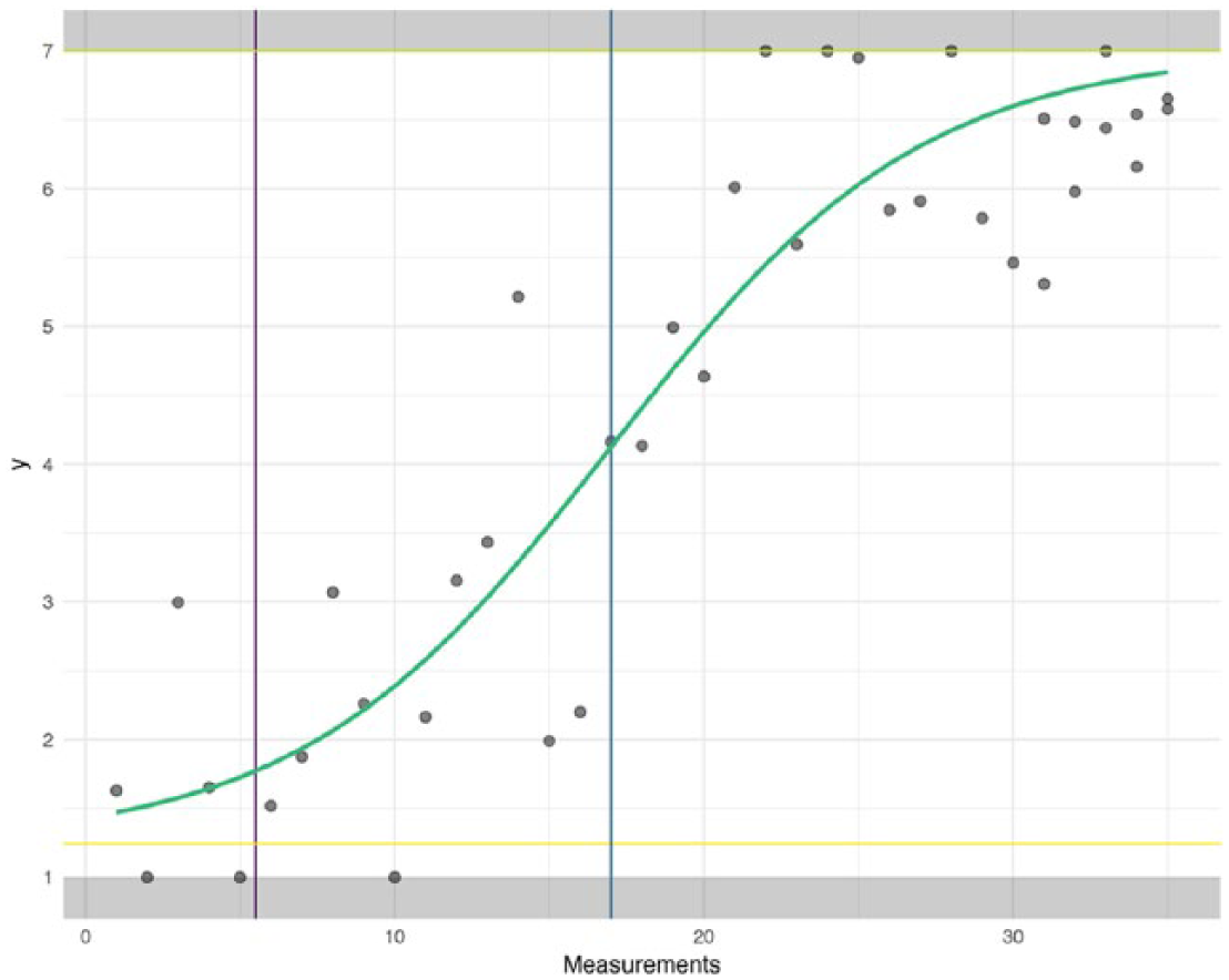
Generalized logistic function fitted to the example data.
At about measurement 17 (12 measurements after the intervention started), the rate of increase in scores is largest. The growth rate is 0.2.
A general effect size could be defined in line with Cohen’s d as follows:

where SD(y) is the SD of y from a particular subject. Instead of the means in both phases, the estimated floor and ceiling are used in this formula. For this example, ES c = 2.75. Alternatively, the theoretical or empirical range of the scale of the measurement instrument could be used in the denominator as
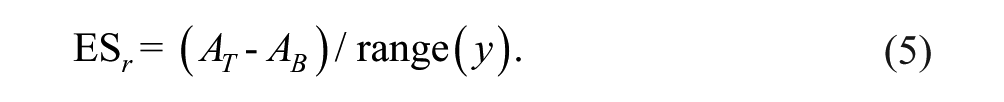
This effect size indicates the proportion of the scale that is improved according to the floor and ceiling of the fit function: in this case, ES r = .96. The growth rate parameter can also be viewed as measure of effect size. An example of six different growth rates is shown in Figure 7. It does not indicate how large an effect is, but how fast the effect is reached. From a practical perspective, it is conceivable that a smaller effect (as measured by ES c or ES r ) that is reached relatively quickly is preferable over a larger effect that takes a long time to be achieved.
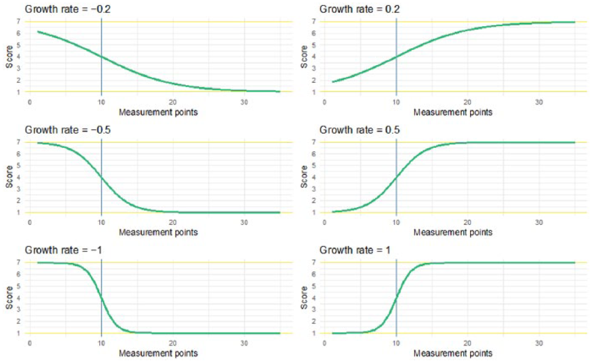
Examples of growth rates for fixed v = 1, x0 = 10, bottom = 1 and ceiling = 7.
The function genlog() has been built around the optimizing function nlsLM() to run the GL model with sensible starting values and minimum and maximum constraints for the parameters (see the appendix or the Open Science Framework repository at https://osf.io/8gcjz/ for a small tutorial, where function piecewiseRegr() is also explained). Sensible starting values and constraints are necessary to avoid convergence problems of the algorithm. The genlog() function also contains the option to plot the result (e.g., Figure 6) using the ggplot2 package (Wickham, 2009), and it is implemented in the userfriendlyscience package (Peters, 2018).
The AT is constrained around the maximum value of the scores of the dependent variable: [max(y)-3, max(y)], AB is constrained around the minimum value of the scores: [min(y), min(y) + 3]. The growth parameter is constrained between −2 and +2. Finally, the inflection point (t0) is constrained between the last-but-two baseline measurement and the last-but-five measurement.
Default starting values for the parameters are for t0 = nA + 4, for AB = min(y), for AT = max(y), and for B = 0. All of the constraints and starting values can easily be changed if the data require other values.
Empirical Examples
Example 1: Singh Data
In their extensive review paper about SCD and methodologies to analyze them, Manolov and Moeyaert (2017a) analyzed a data set from Singh et al. (2007), see Figure 8. In this article, we will also use these data to illustrate the GL model and compare the results with those presented in the Manolov and Moeyaert paper. The data were obtained from three individuals measuring their verbal and physical aggression before and after an intervention, which consisted of mindfulness training for controlling aggressive behavior. The individuals were diagnosed with several mental disorders such as depression, schizoaffective disorder, borderline personality, and antisocial personality. These data are considered representative for single case data in the literature (Shadish & Sullivan, 2011).
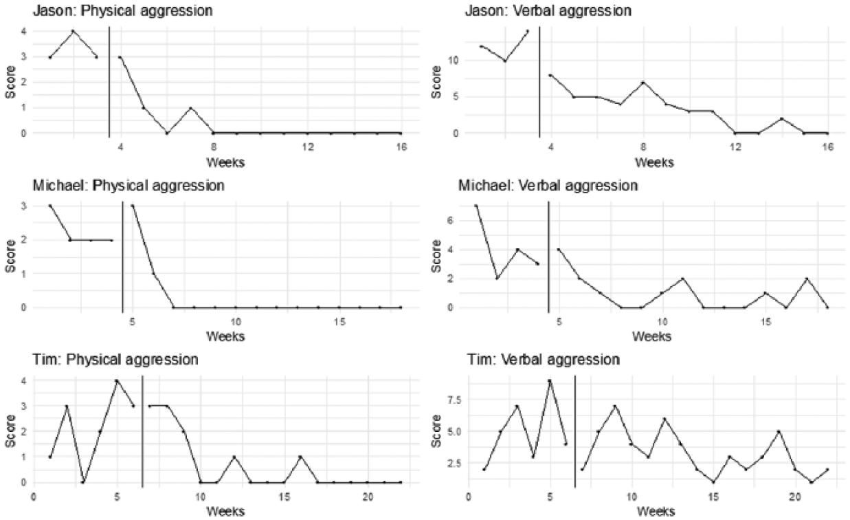
Representation of the six data sets obtained from Singh et al. (2007).
In Table 1, the results are presented of the three effect size statistics and the deviance obtained from the GL analyses and these are compared with the effect size measures of the PWR analysis and Cohen’s d (see also Manolov & Moeyaert, 2017b). Cohen’s d only compares the level effect between the two phases, PWR compares both level and linear trend, and GL fits a curved effect.
Comparison of Fit Measures and Effect Sizes Between GL, PWR, and Cohen’s d.
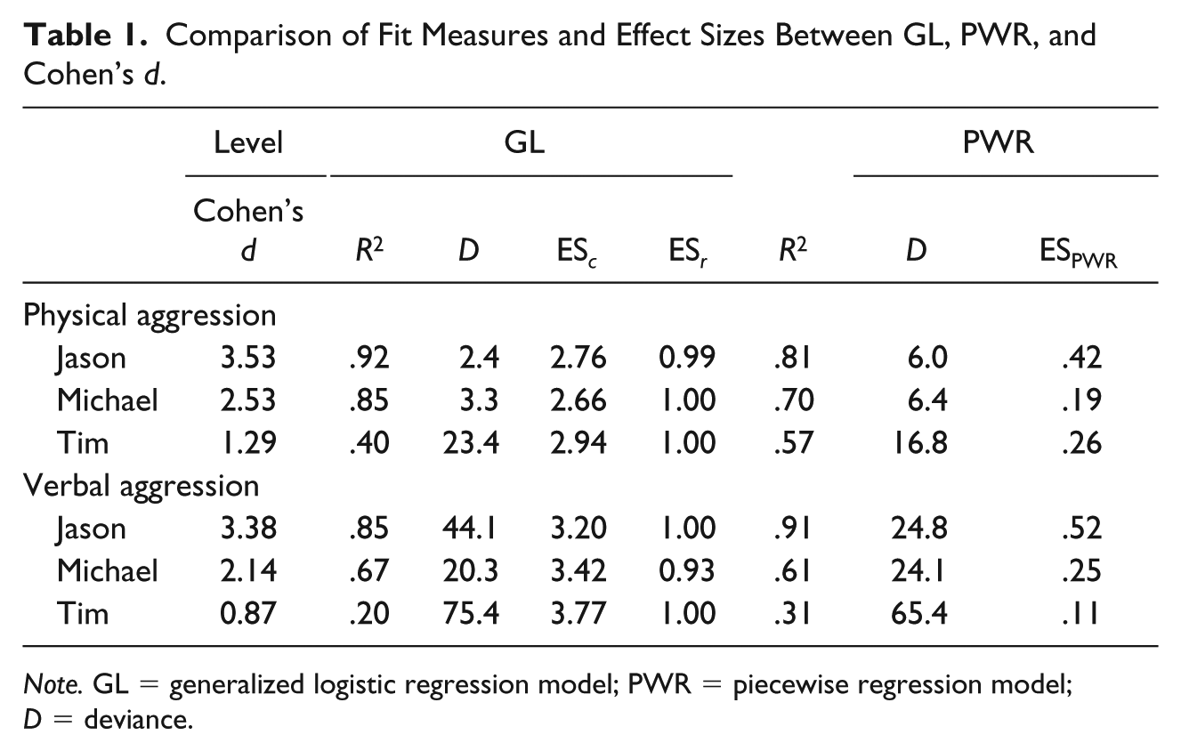
Note. GL = generalized logistic regression model; PWR = piecewise regression model; D = deviance.
The question we want to answer in this example is whether the most important characteristics in Figure 9 are captured by the fit measures. Does the information obtained from fitting the GL model provide us with another kind of insight compared with the PWR or Cohen’s d. The answer for this question, we look at the fit values and effect sizes (Table 1) and to the parameter estimates (Table 2) of both analysis techniques.
Comparison of the Model Parameters Between GL and PWR Model.
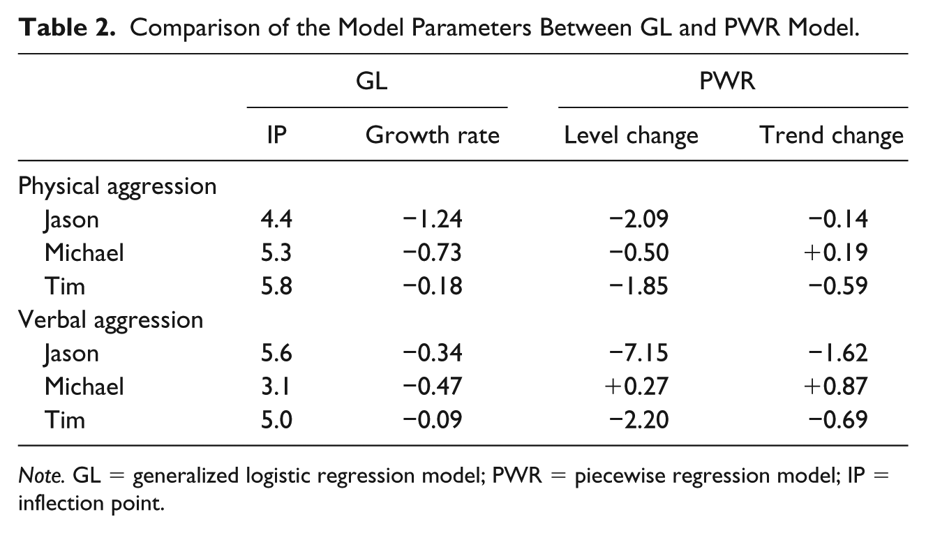
Note. GL = generalized logistic regression model; PWR = piecewise regression model; IP = inflection point.
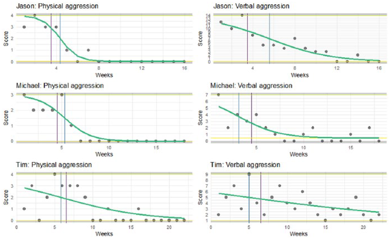
Data from Singh et al. (2007) analyzed with the GL model.
From visual inspection, we learn that Jason has made the biggest improvement, both with respect to verbal and physical aggression. However, this effect is based on only three measurements in the baseline phase. First we notice that the R2 (Table 1) indicates that the GL model can very well summarize Jason’s data: it is even larger than the large R2 of the PWR model. Despite the low number of data points in the first phase, the effect in Jason’s data is well captured by the growth rate, see Table 2. Aggressive behavior improves (i.e., decreases) most quickly shortly after the intervention commences, as indicated by the inflection point parameter. This is supported by the visual inspection, in particular for physical aggression.
Both Tim’s aggression behaviors are fitted less well than the other subjects’ behaviors. This is true for GL and PWR, but GL fits slightly worse than PWR as can be seen from the R2 and the deviances in Table 1. PWR shows rather large trend and level ES for Tim, contrary to GL that indicates that the growth rate is much less than that of the other persons. In all cases, the floor and ceilings parameters are in line with what should be expected when we visually inspect the data.
ES c is difficult to interpret: there seems no obvious relation with the visual characteristics. The GL model shows only small differences between the effect sizes of the three subjects, contrary to Cohen’s d and the PWR model. Especially the effect sizes for Tim are small according to PWR and Cohen’s d, but the GL model finds an effect size that appears even somewhat larger than for the other two subjects.
The ES r for physical aggression is equal for Jason and Tim, which arguably makes sense when we look at the data. However, PWR indicates that the effect for Jason is much larger than for Tim. The difference can be explained by measurements 6 to 8 which are rather high and are in the postintervention phase. For PWR, this decreases the effect size, whereas for GL this merely moves the inflection point further away from the phase shift. This differential influence on the analysis outcome is important to take into consideration when deciding which approach to use.
Example: Sex Therapy Data
The data for this example were obtained from a study about the effectiveness of sex therapy (van Lankveld, Leusink, & Peters, 2017). The data are from a single person who provided scores on several variables at 38 time points during a year. The measurement points were not equally spaced in time. During the baseline period, a measurement was obtained every few days, after which the intermeasurement intervals were gradually increased to up to a month at the end of the study. Because dates were available for each measurement, it was possible to take these differential intervals into account when modeling the treatment effects.
In this example, we will show three of the eight variables that were measured in this study, specifically self-esteem, intimacy toward the partner and experience of masturbation. The GL and PWR model were used to analyze these variables. The relevant output of the GL analysis of the three variables is presented in Table 3.
Result of the Analyses of the Sex Therapy Data by the GL Model.
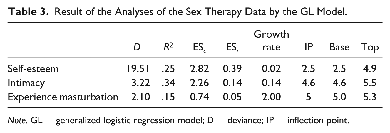
Note. GL = generalized logistic regression model; D = deviance; IP = inflection point.
For the variable self-esteem, the deviance compared with the PWR is slightly better (Dpw = 18.6), while the R2 is slightly smaller (
The therapy effect size for self-esteem is larger than for the other two variables. Figure 10 demonstrates the results graphically. We zoomed in on the small effects for intimacy and masturbation experience (note the small range on both y axes) to illustrate the sigmoid curve. Although the effect is small, the GL suggests that an effect takes place immediately at the start of the therapy. After the initial improvement the function flattens and during the rest of the therapy period no further improvements are made.
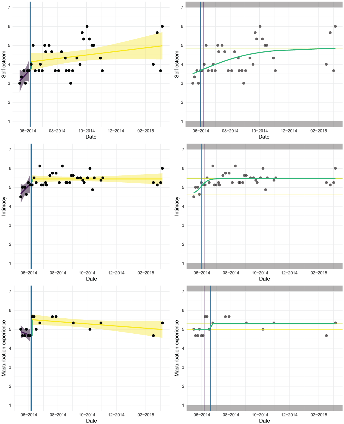
Analyses of self-esteem, intimacy, and experience of masturbation in sex therapy study.
For self-esteem, the GL model does not appear to be appropriate, as the fitted curve is almost a straight line. The PWR model seems more appropriate here although the fit values are also quite low.
In analyzing these data, we found that changing the start and boundary values may influence the outcomes. A small change in start values may result in a different curve. This implies that the optimization process for fitting the GL suffers from local minima. To explore the influence of local minima one should run a sensitivity analysis. This can be done by simply setting different start values and then inspect the fit and effect sizes. The analysis yielding the largest fit with the data should then be taken as the preferred one. In the appendix, we provide visual tools to inspect how the default and tweaked values for the start values of the parameters influence the resulting estimates.
Discussion
This article discusses a new method to analyze experimental single case data based on a generalized logistic model. The underlying assumption of this method is that intervention effects represent the shift of an individual’s scores from one plateau to another, and that the individual’s scores are limited by floors and ceilings, which are caused by the measurement instrument and by natural limits of the process under study. This implies that the linear models to estimate the intervention effect are at best suboptimal because their assumptions are violated, and, relatedly, they fit the data poorly. The generalized logistic model seems better equipped to deal with these floor and ceiling aspects of the measurement instruments. Another new aspect in this model is the estimation of the onset and the end of the intervention effects.
To test the proposed method we built the R function genlog around a general existing optimizing function, with this new function providing sensible default starting values and constraints. Running the genlog function yields parameter estimates and also provides visualization of the data and the fitted function. Together with the function we proposed two simple effect size measures derived from Cohen’s d. In addition, we argued that the growth parameter of the function could serve as an additional effect size measure, indicating the speed of the intervening process. How to qualify the effect size we proposed as large or small is a question that remains to be addressed (see also Manolov, Gast, Perdices, & Evans, 2014). Visual inspection of the data was used here to gauge the plausibility of our effect sizes. More studies are necessary to obtain a better understanding of these effect sizes.
Based on a well-known single case data (Singh et al., 2007), we illustrated the generalized logistic model. The Singh data are also discussed in Manolov and Moeyaert (2017a) and used to compare a wide variety of single case methods. The model was applied to these data and compared with the PWR model. The generalized logistic model provided sensible outcomes that seem to add to the understanding of the intervention process. Based on these analyses, we recommend that one should combine the result of the model fit with that of the estimated growth parameter and the second effect size, which is based on the range of the data, to obtain informative outcomes.
A second example (van Lankveld et al., 2017) also illustrated that the generalized logistic model can be helpful in analyzing the data. On the contrary, this example also made it clear that in some situations given start and boundary values can be very influential. The parameter estimates of the generalized logistic model are not robust in the sense that they depend on parameter constraints and starting values. With relatively few data points and four parameters to estimate this is not surprising. Fixing the top and ceiling values after visual inspection can improve the robustness of the remaining parameters. We also recommend to run sensitivity analyses to explore to what extent the outcomes depend on the start values of the optimization process.
For valid interpretation of the GL results, we recommend to first inspect the deviance and the R2. If the R2 is low and the deviance is high, the curve cannot fit the data well and all ES values are most likely rather meaningless. Keep in mind that in SCD, the R2 values are usually larger than in “classical” regression situations with large N, as there are a limited number of data points in SCD.
When the data contain many discontinuities, for instance scores go up and down several times, other approaches, such as PWR splines, are flexible alternatives for fitting the data. Splines are more general, because they could fit discontinuities, which might be a necessary property for fitting data that show complex patterns. However, for the generalized logistic model we assume situations, such as therapy situations, in which there is a more or less gradual increase (cq decrease) in behavior or attitude. Furthermore, flexible cubic splines need more parameters to estimate than the GL model, which may become problematic when there are only a small number of data points as is common in single case research (James, Witten, Hastie, & Tibshirani, 2013). Finally, the interpretation of the coefficients from the spline approach is more complex than for the GL model.
With multiple single case data (i.e., replicated n-of-1 designs), future research should focus on whether this model can be incorporated in a multilevel context. In Baek et al. (2014), the integration of single case results by multilevel analyses is discussed. It is shown by these authors how the PWR model can be incorporated in a multilevel framework. Moeyaert, Ugille, Ferron, Beretvas, and Van den Noortgate (2014) found empirical evidence that the fixed effects in three level analyses of single case studies are unbiased, a result that was found earlier in two level analysis (Ferron, Bell, Hess, Rendina-Gobioff, & Hibbard, 2009). It was also found by combining more than 30 studies that the mean squared error was hardly influenced by the small SCDs. It is expected that this finding generalizes to the model we have proposed in the present study. Combining many studies has the additional advantage that the estimated model parameters will show more robustness (i.e., be less dependent on the starting values).
In this article, we have presented another tool to add to the already wide collection of SCD approaches (Manolov & Moeyaert, 2017b). It is based on the idea that most effects of interventions have a natural limit. Based on this simple premise, we have proposed a model that would represent this idea. The software we have presented is Free and Open Source Software, implemented in the popular statistical environment R, and easy to apply, with some additional support in a short tutorial (see the appendix and https://osf.io/8gcjz/?view_only=5b7a3c11bf8d4fe7a85410ad0a3d1447)
Supplemental Material
Appendix__applying_the_generalised_logistic_model_in_single_case_designs__modelling_treatment-induced_shifts_(1) – Supplemental material for Applying the Generalized Logistic Model in Single Case Designs: Modeling Treatment-Induced Shifts
Supplemental material, Appendix__applying_the_generalised_logistic_model_in_single_case_designs__modelling_treatment-induced_shifts_(1) for Applying the Generalized Logistic Model in Single Case Designs: Modeling Treatment-Induced Shifts by Peter Verboon and Gjalt-Jorn Ygram Peters in Behavior Modification
Footnotes
Declaration of Conflicting Interests
The author(s) declared no potential conflicts of interest with respect to the research, authorship, and/or publication of this article.
Funding
The author(s) received no financial support for the research, authorship, and/or publication of this article.
Supplemental Material
Supplemental material for this article is available online.
Author Biographies
References
Supplementary Material
Please find the following supplemental material available below.
For Open Access articles published under a Creative Commons License, all supplemental material carries the same license as the article it is associated with.
For non-Open Access articles published, all supplemental material carries a non-exclusive license, and permission requests for re-use of supplemental material or any part of supplemental material shall be sent directly to the copyright owner as specified in the copyright notice associated with the article.