Sage Journals: Discover world-class research

Abstract

The problem of uncertainty in wind turbines is caused by factors like the random and stochastic nature of the wind, variations in the moment of inertia of its rotating parts, damping, stiffness factors, and discrepancies between its actual and mathematical model. The presence of uncertainty would deteriorate the wind turbine's performance, which can significantly affect rotor speed. Therefore, robust control strategies for speed control are necessary in the presence of uncertainties and wind disturbances, with the help of the control input taken as the blade pitch angle. Hence, a robustly stabilizing proportional-integral (PI) controller is designed under the purview of Kharitonov's polynomials to control the rotor speed for a ± 25% uncertain multi-input wind turbine. The robustly stabilizing (K_p, K_i) region of the designed PI controller is obtained by Kharitonov's theorem based on the 16-plant model after the formation of Kharitonov's rectangles. A (K_p, K_i)-subregion is also extracted for all plants individually to achieve the desired time response specifications. The purpose of this analysis is to make sure that a simple PI controller can be made robust when there is a provision to choose its parameters from the stabilizing regions achieved. Real-time simulations are also made on the OPAL RT OP5700 Simulator to validate the performance of robust controllers designed in MATLAB. The real-time results clearly validate the performance of robustly designed controllers.

Keywords

Robust control uncertainty modeling multi-input systems wind turbines real-time simulations

Introduction

A single large contemporary wind turbine (WT) may generate several megawatts, which are expensive, need regular maintenance, and must endure harsh weather conditions, primarily variations in wind speeds. The significant increase in wind energy, viz., large WT, imposes challenges to the control domain's perspective owing to the unmodelled dynamics of the WT, fatigue, aerodynamics, structural analysis, and turbulence (El Beshbichi et al., 2023), (Adeoye et al., 2024), (Metwally Mahmoud, 2023). These factors sum up to create uncertainty in the WT (Salem et al., 2017), (Mahmoud et al., 2022b), (Boudjemai et al., 2023b). A model called stochastic network-constrained unit commitment (NCUC), as introduced in the work (Naghdalian et al., 2020), has been developed. By considering the required flexible ramp and spinning reserves in the face of demand and wind power uncertainty, it seeks to determine the optimal daily plan for generating units.

Research has been carried out invariably in the control aspects of WTs (Mahmoud et al., 2023b), (Mahmoud et al., 2023a), (Boudjemai et al., 2023a), (Aldin et al., 2023). The risk of failures increases in the modern power system dynamics due to increased use of renewables, and hence, must account for frequency control to detect grid power imbalances (Kheshti et al., 2020), (Atia et al., 2024). The blade pitch control system is designed for wind systems (Mahmoud et al., 2022a), which discusses the fundamental construction of WTs, control loops, controllers, and their latest advancements. A review on the control of WTs to improve their performance based on desired objectives encompassing cost reduction, increased energy capture, and the combination of both is presented (Apata and Oyedokun, 2020). The variable speed WTs were controlled by controlling the blade pitch angle (Bahmani et al., 2020). It is used primarily under strong wind currents to limit power extraction from wind energy. Pitch control is possible in two ways: control of combined pitch and control of individual pitch. The latter is used in large WTs to restrict the output under strong winds (Hamoodi et al., 2020), (Boudjemai et al., 2025). A novel strategy using adaptive fuzzy logic is developed for improved performance of turbine-generator systems for wind energy extraction (Soliman et al., 2019), (Menzri et al., 2024).

In (Rigatos and Siano, 2011), a power system stabilizer is suggested that is built in a simulated setting using the extremal gain-margin theory of Kharitonov. It stabilizes a small number of extreme plants, which results in the design of a controller having low order and exhibiting the characteristics of a phase-lead compensator that is resistant to operating point changes. A robust controller to damp out the oscillations during the wind power generation is considered in (Isbeih et al., 2019), (Boutabba et al., 2025). An effective strategic approach known as an integral backstepping strategy (IBS) is applied on a variable-speed generator for optimal power extraction by the WT (Saidi et al., 2021). By using this control mechanism, the mechanical stress on the WT and generator shafts is reduced. A decoupled PI current controller is designed for WTs sourcing an inverter tied to the grid (Errouissi et al., 2018).

This work outlines the design of a PI controller aimed at stabilizing a range of interval plants (Matušů, 2011). Additionally, it offers a thorough evaluation of every stabilizing PI controller appropriate for this kind of interval plant family. In (Petkov et al., 2018), the authors developed a robust controller for a model that was uncertain, which includes the design of three robust controllers, namely H_∞−, µ-, and loop shaping. The authors in (Bhattacharyya, 2017) delved into the topic of robust control in the presence of parametric uncertainty.

The disturbances in power quality are compensated to overcome the problem of uncertainty in renewable generation at the point of common coupling (Chishti et al., 2020). The harmonics produced due to the nonlinear component of load current are filtered by a robust, normalized, mixed-norm adaptive algorithm. A sliding mode controller for a doubly-fed induction generator-based WT was explored to regulate the speed and the generated power in the presence of uncertainties (Jafari and Shahgholian, 2017). Similarly, a second-order sliding mode controller was explored to optimize the generation of power by a WT (Liu et al., 2017). During the design of a WT model for analysis, there is a chance of neglecting the environmental conditions and working parameters (Cascianelli et al., 2022), (Huang et al., 2020) upon which the production of power by a WT depends. The potential danger to WT stability and performance under the effect of uncertainties has gained importance, and is thus the subject of this paper's examination. The control strategies for industrial wind turbines are the PID regulators (Habibi et al., 2018), (Fayz et al., 2025). By embedding a Nussbaum-type function with a novel PID-based fault-tolerant controller, a robust adaptive control scheme is developed for WTs. The Kharitonov-based PI controller, as described in (Asadi, 2018), is widely used for modeling a 16-plant model derived from a specified interval plant. This method is employed to establish a suitable stabilizing region for the values of K_p and K_i, including their Kharitonov rectangles. Several researchers have provided in-depth insights into Kharitonov-based controllers, such as the 16-plant theorem (Toulabi et al., 2018), as well as the development of robust PID controllers (Chu and Chu, 2018), (Vo, 2018). The high-cost, large WTs with inevitable uncertainties need proper controllers; otherwise, the loss can be irreparable. Hence, the focus is typically on active management of bigger flexible WTs that are prone to uncertainties, to decrease the losses, viz., economic and structural, otherwise, it might lead to costly compensation (Wang et al., 2018). This discusses the necessity of designing a controller for a WT that incorporates uncertainty modeled using Kharitonov's polynomial, which can control the generator's speed using blade pitch angle control.

This study presents a unique control approach for a multi-input uncertain WT exposed to ±25% uncertainty. The technique is centered on attaining a stabilizing area relating to a set of controller gains (K_p, K_i). It is found that the performance of the uncertain WT may be reliably stabilized with any set of gains. But to meet the desired time response specifications, sub-regions for all 16 individual plants were also achieved. The performance of the uncertain WT may be securely stabilized in the presence of wind disturbance with any combination of gains selected from the different sub-regions. Moreover, these performances of all individual controllers are validated in a real-time environment (OPAL RT OP5700) by simulating all 16 controlled plants to consolidate the robustness of controllers designed using Kharitonov's 16 plant theorem.

The paper's structure is as follows: Section 1 covers the introduction to wind energy, types of wind turbines, potential dangers to wind turbine stability and performance, uncertainties in wind turbines, and the control methods to deal with an uncertain WT. In Section 2, a linearized WT model with seven states is shown. In Section 3, a WT model under the presence of uncertainty is modeled. A PI controller is designed based on Kharitonov's polynomials, the mathematical preliminaries of which are presented in Section 4. The 16-plant model is used to illustrate the resilient controller design in Section 5, while the simulation results for the uncertain WT model are presented in Section 6. Lastly, section 7 presents the conclusions.

WT mathematical model

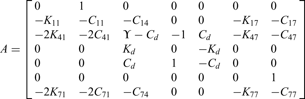
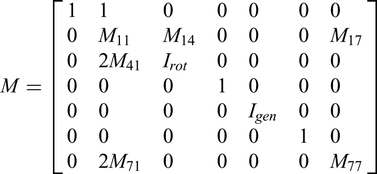
This section presents the WT mathematical model, which was adapted in (Wright and Balas, 2003). It is a two-bladed, 600 kW, upwind machine having it's a rotational speed of 42 rpm. The seven-state linearized WT's state-space representation may be expressed as:

M x (\dot{t}) = A x (t) + B u (t) + Γ u_{d} (t)

(1)

y (t) = C x (t)

(2)

where M represents mass matrix ∈ R⁷ ^× ⁷, x(t) represents the state vector ∈ R⁷ ^× ¹, A represents the system matrix ∈ R⁷ ^× ⁷, and B represents the input matrix ∈ R⁷ ^× ¹, Γ represents the disturbance input matrix ∈ R⁷ ^× ¹, C represents the control input gain matrix ∈ R¹ ^× ⁷, u(t) represents the controlled input (blade pitch angle), β and u_d(t) represents the disturbance input (wind) and y(t) represents the output vector.

The seven-states considered in equation (1) are namely: rotor blade displacement (x₁(t)), rotor blade velocity (x₂(t)), rotational speed of the rotor (x₃(t)), torsional force (x₄(t)), rotational speed of the generator (x₅(t)), tower's deflection (x₆(t)) and tower's velocity (x₇(t)). The constants M_ij, K_ij, and C_ij represent mass-elements, stiffness-elements, and damping-elements, respectively (i and j take values from 1 to 7), ζ functions as a partial derivative of the aerodynamic torque of the rotor considering changes in β. I_rot and I_gen denote the rotor and generator's moments of inertia, while K_d and C_d represent the damping and stiffness components, respectively. These matrices are given below.

A = [\begin{matrix} 0 & 1 & 0 & 0 & 0 & 0 & 0 \\ - K_{11} & - C_{11} & - C_{14} & 0 & 0 & - K_{17} & - C_{17} \\ - 2 K_{41} & - 2 C_{41} & Υ - C_{d} & - 1 & C_{d} & - K_{47} & - C_{47} \\ 0 & 0 & K_{d} & 0 & - K_{d} & 0 & 0 \\ 0 & 0 & C_{d} & 1 & - C_{d} & 0 & 0 \\ 0 & 0 & 0 & 0 & 0 & 0 & 1 \\ - 2 K_{71} & - 2 C_{71} & - C_{74} & 0 & 0 & - K_{77} & - C_{77} \end{matrix}]

M = [\begin{matrix} 1 & 1 & 0 & 0 & 0 & 0 & 0 \\ 0 & M_{11} & M_{14} & 0 & 0 & 0 & M_{17} \\ 0 & 2 M_{41} & I_{r o t} & 0 & 0 & 0 & 0 \\ 0 & 0 & 0 & 1 & 0 & 0 & 0 \\ 0 & 0 & 0 & 0 & I_{g e n} & 0 & 0 \\ 0 & 0 & 0 & 0 & 0 & 1 & 0 \\ 0 & 2 M_{71} & 0 & 0 & 0 & 0 & M_{77} \end{matrix}]

C = [\begin{matrix} 0 & 0 & \begin{matrix} 0 & 0 & \begin{matrix} 1 & 0 & 0 \end{matrix} \end{matrix} \end{matrix}]

B = {[\begin{matrix} 0 & α_{b} & \begin{matrix} 0 & 0 & \begin{matrix} 1 & 0 & 0 \end{matrix} \end{matrix} \end{matrix}]}^{T}

Γ = {[\begin{matrix} 0 & β_{b} & \begin{matrix} β & 0 & \begin{matrix} 1 & 0 & β_{t} \end{matrix} \end{matrix} \end{matrix}]}^{T}

The standard state space form is obtained by rewriting equations (1) and (2).

x (\dot{t}) = M^{- 1} A x (t) + M^{- 1} B u (t) + M^{- 1} Γ u_{d} (t)

(3)

y (t) = C x (t)

(4)

Equation (3) is rewritten as

x (\dot{t}) = \bar{A} x (t) + \bar{B} u (t) + \bar{Γ} u_{d} (t)

(5)

y (t) = C x (t)

(6)

where,

\bar{A} = M^{- 1} A, \bar{B} = M^{- 1} B, \bar{Γ} = M^{- 1} Γ, a n d \bar{C} = C

The uncertain WT model

Uncertainties are inevitable in real-time systems, and they are particularly apparent in the functioning of WTs. The uncertainty may be categorized into three types: disturbances due to fluctuations in wind speed, noise from measurement processes, and dynamic perturbations arising from variations between the plant's mathematical model and its real-time operational dynamics. Unmodeled dynamics due to high frequencies, the nonlinearities that were ignored during modeling, parameter variations in the system due to changing climatic conditions, and wear and tear factors can all cause dynamic perturbations in WTs. These factors can adversely affect the performance and stability of the control system.

As illustrated in Figure 1, the dynamic perturbations are grouped in a block and are known as the uncertainty matrix (Δ). It is also represented by Δ(s) the uncertainty transfer function. Here, Gpert(s), which is defined by equation (7), represents the real dynamics of a perturbed WT (the dotted block in Figure 1).

G p e r t (s) = G_{W T} (s) + Δ (s)

(7)

where G_WT (s) represents the nominal WT's transfer function and Δ(s) represents the structured uncertainty [3] given by equation (8)

Δ = d i a g [δ i a i]

(8)

where i = 1, 2, 3,… 21 elements for which ±25% uncertainty is introduced, a′ ′s are the elements of the system matrix, while the relative changes in these elements are represented by δi. In this paper, a robust stabilizing controller (PI) based on a 16-plant model of Kharitonov's theorem is proposed, which can control the blade pitch angle and speed of the generator of an uncertain WT for random variations in wind velocities.

Figure 1.

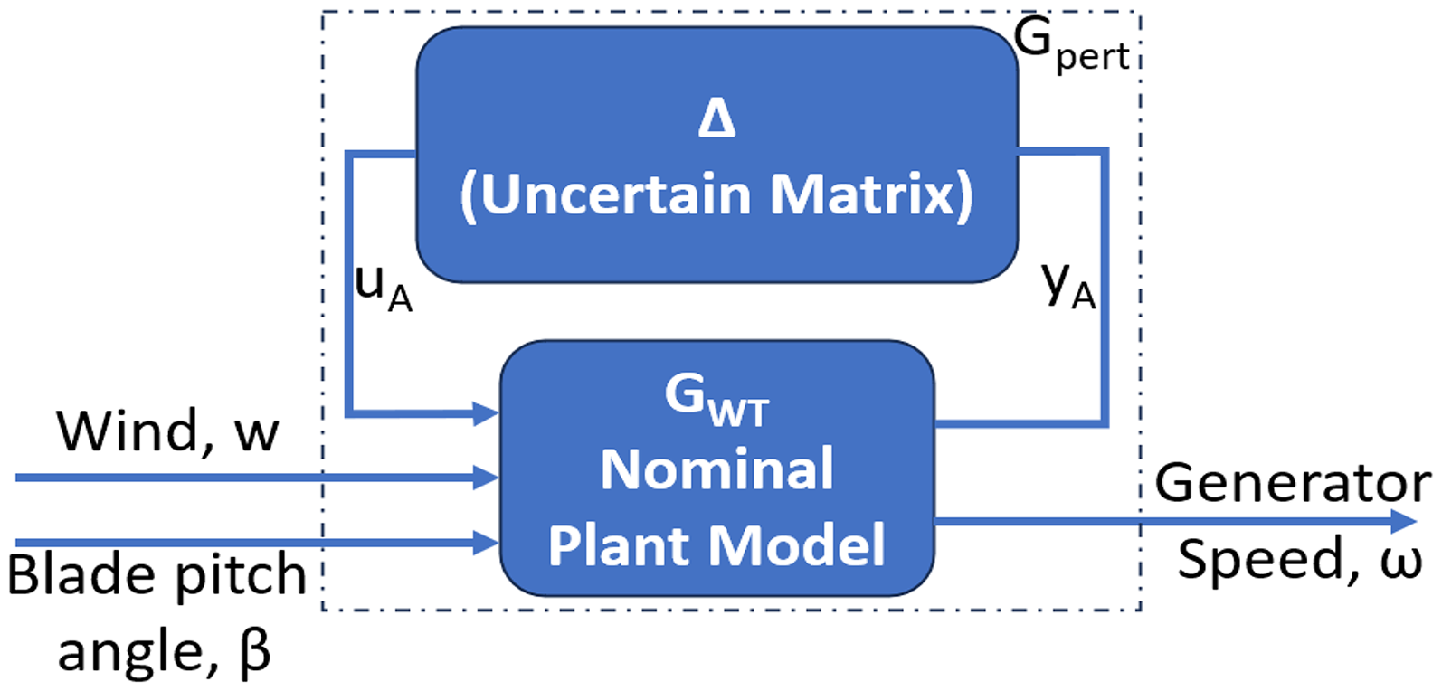
A block diagram of an uncertain wind turbine.

Kharitonov's theorem preliminaries

Stability analysis typically involves the Routh-Hurwitz stability test, which applies to fixed polynomials. However, when dealing with polynomials featuring uncertain coefficients, stability analysis can be effectively carried out using Kharitonov's theorem. Two main methods are used to evaluate polynomial stability, which are, for a particular polynomial or family of polynomials, by locating the roots in the left half of the s-plane, and by considering limitations on the polynomial or polynomial family, such as damping factor or settling time. All roots of the specified family of polynomials must exist inside the region, a subset in the left half of the s-plane, to guarantee stability (Asadi, 2018).

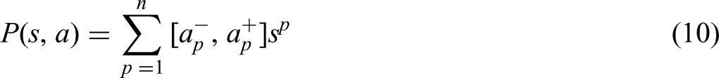
Def: The interval polynomial is a polynomial family defined by

P (s) = a_{0} + a_{1} s^{1} + a_{2} s^{2} + \dots \dots \dots \dots + a_{n} s^{n} = \sum_{p = 0}^{n} a_{p} s^{p}

(9)

∀p, where a_p ∈ [l_p, u_p] and 0 ∈/ [l_p, u_p]. The boundaries (both minimum value and maximum value) of the p^th coefficient are represented by l_p and u_p, respectively, and the order of the polynomial P (s) is denoted by n.

The minimum value and maximum value given by the general equation (10) yield four predefined Kharitonov's polynomials given by (Asadi, 2018), (Vo, 2018):

P (s, a) = \sum_{p = 1}^{n} [a_{p}^{-}, a_{p}^{+}] s^{p}

(10)

Therefore, the fixed polynomials are expressed as equation (11).

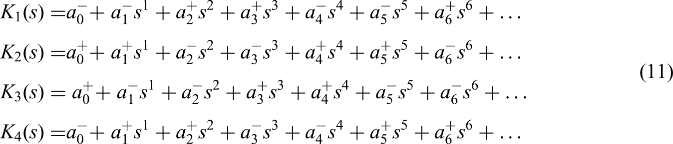
\begin{aligned} K_{1} (s) = & a_{0}^{-} + a_{1}^{-} s^{1} + a_{2}^{+} s^{2} + a_{3}^{+} s^{3} + a_{4}^{-} s^{4} + a_{5}^{-} s^{5} + a_{6}^{+} s^{6} + \dots \\ K_{2} (s) = & a_{0}^{+} + a_{1}^{+} s^{1} + a_{2}^{-} s^{2} + a_{3}^{-} s^{3} + a_{4}^{+} s^{4} + a_{5}^{+} s^{5} + a_{6}^{-} s^{6} + \dots \\ K_{3} (s) = & a_{0}^{+} + a_{1}^{-} s^{1} + a_{2}^{-} s^{2} + a_{3}^{+} s^{3} + a_{4}^{+} s^{4} + a_{5}^{-} s^{5} + a_{6}^{-} s^{6} + \dots \\ K_{4} (s) = & a_{0}^{-} + a_{1}^{+} s^{1} + a_{2}^{+} s^{2} + a_{3}^{-} s^{3} + a_{4}^{-} s^{4} + a_{5}^{+} s^{5} + a_{6}^{+} s^{6} + \dots \end{aligned}

(11)

According to Kharitonov's Theorem, the four fixed Kharitonov polynomials must be stable in order to achieve an interval polynomial family, P (s, a), that is robustly stable (Asadi, 2018).

Lemma: The following properties must be true for an n^th order interval polynomial given by (10) to be robustly stable (Asadi, 2018). They are:

− stable K₃(s) when n = 3

− stable K₂(s) and stable K₃(s) when n = 4

− stable K₂(s), stable K₃(s) and stable K₄(s) when n = 5

− stable K₁(s), stable K₂(s), stable K₃(s) and stable K₄(s) when n ≥ 6

Formation of 16 Kharitonov plants

Upon introduction of ±25% uncertainty for the aforementioned 21 system matrix elements in Section 3, an uncertain family of polynomials is formed for both the numerator and denominator pertaining to the nominal transfer function given by equation (12).

P (s, a, b) = \frac{N (s, a)}{D (s, b)} = \frac{\sum_{p = 0}^{m} [a_{p}^{-}, a_{p}^{+}] s^{p}}{s^{n} + \sum_{p = 0}^{n - 1} [b_{p}^{-}, b_{p}^{+}] s^{p}}

(12)

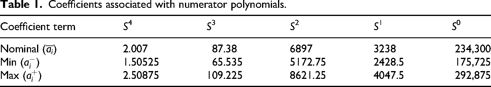
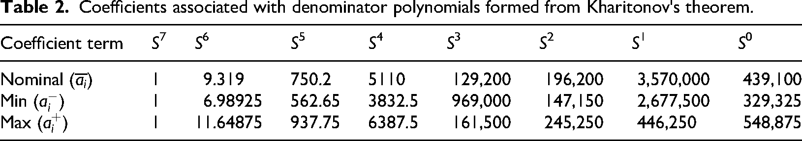
The equation (12), P (s, a, b), should be proper strictly. Four Kharitonov's polynomials are then produced by the numerator and denominator polynomials, respectively. Tables 1 and 2 are formed because of the application of ±25% uncertainty, respectively, to the 21 system matrix elements, yielding lower and upper bounds.

Table 1.

Coefficients associated with numerator polynomials.

Coefficient term	S ⁴	S ³	S ²	S ¹	S ⁰
Nominal ( $\bar{a_{i}}$ )	2.007	87.38	6897	3238	234,300
Min $(a_{i}^{-})$	1.50525	65.535	5172.75	2428.5	175,725
Max $(a_{i}^{+})$	2.50875	109.225	8621.25	4047.5	292,875

Table 2.

Coefficients associated with denominator polynomials formed from Kharitonov's theorem.

Coefficient term	S ⁷	S ⁶	S ⁵	S ⁴	S ³	S ²	S ¹	S ⁰
Nominal ( $\bar{a_{i}}$ )	1	9.319	750.2	5110	129,200	196,200	3,570,000	439,100
Min $(a_{i}^{-})$	1	6.98925	562.65	3832.5	969,000	147,150	2,677,500	329,325
Max $(a_{i}^{+})$	1	11.64875	937.75	6387.5	161,500	245,250	446,250	548,875

Kharitonov's theorem introduces the 16-plant theorem, which involves obtaining Kharitonov polynomials for the numerator and denominator separately, i.e., N₁(s), N₂(s), N₃(s) and N₄(s) and D₁(s), D₂(s), D₃(s) and D₄(s) (Asadi, 2018). Hence, according to equation (13), the 16 Kharitonov plants are obtained as follows: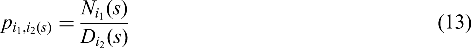

p_{i_{1}, i_{2} (s)} = \frac{N_{i_{1}} (s)}{D_{i_{2}} (s)}

(13)

where i₁, i₂ ∈ 1, 2, 3, 4

Kharitonov's rectangles

A rectangle is formed from the four fixed polynomials given in equation (11) for a given value of ω. The value of ω is varied in steps from 0 to ω₀ to obtain a set of rectangles known as Kharitonov's rectangles. According to the zero exclusion principle (Asadi, 2018), the location of origin in the complex plane should lie out of range with the locus of rectangles, and the same is achieved as shown in Figure 2; then the four determined polynomials are said to be stable.

Figure 2.

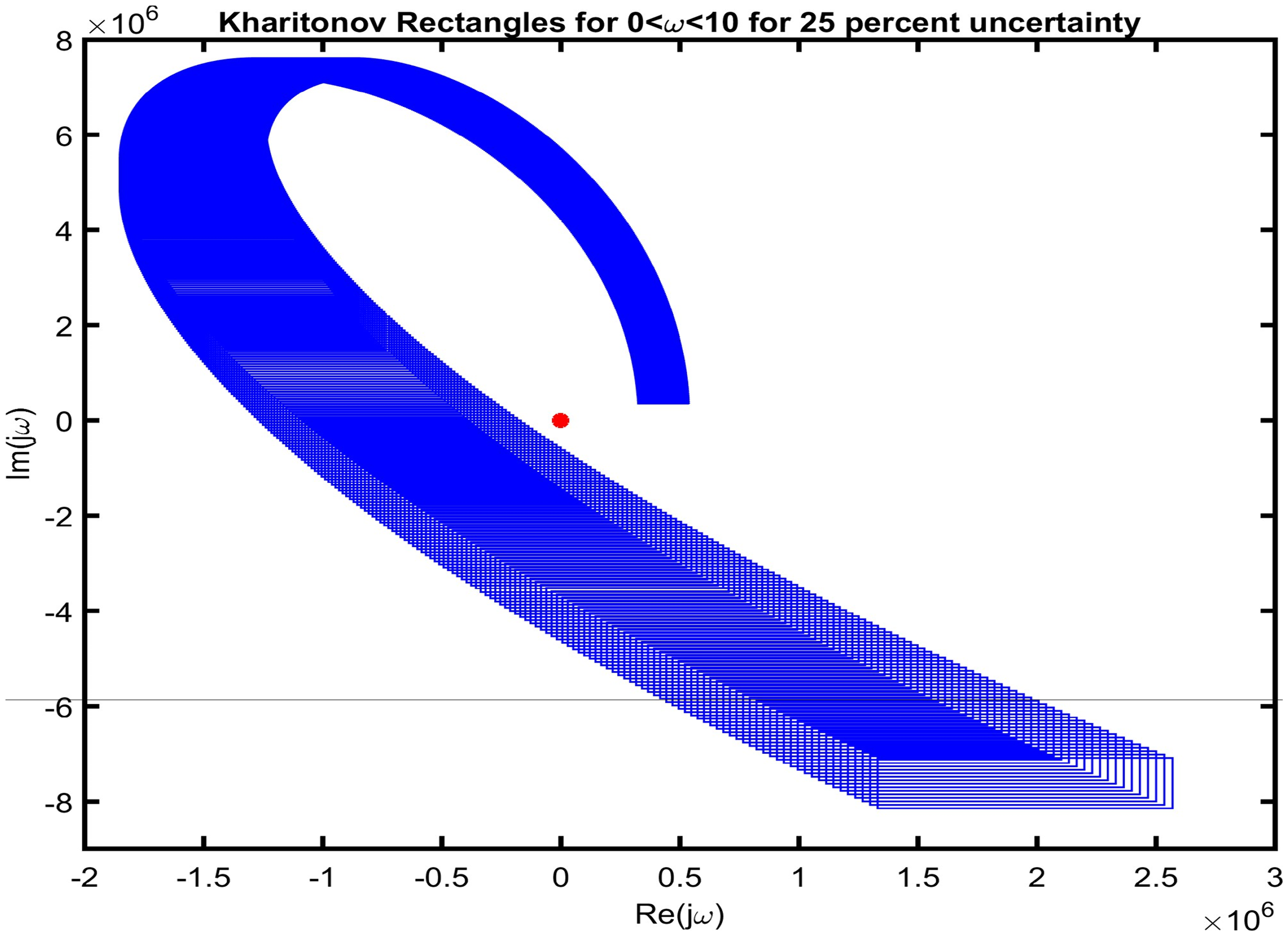
Kharitonov's rectangles validating the zero-exclusion principle. The red asterisks signify that the origin lies outside the set of rectangles, indicating stability.

The robust controller design methodology utilizing a 16-plant model

The control scheme illustrated in Figure 3 depicts a robustly stabilizing PI controller designed for an uncertain wind turbine, employing Kharitonov's theorem (16-plant model approach). The goal of this PI controller design is to stabilize all members of the polynomial family defined by P (s, a, b).

Figure 3.

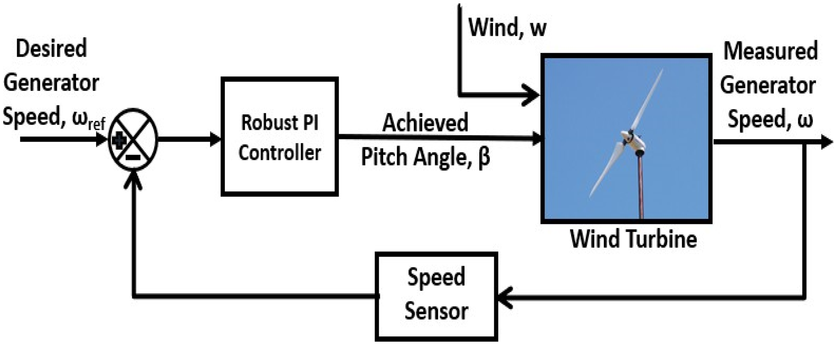
Control feedback for an interval plant P (s, a, b).

Procedure for designing suitable gains for the controller

The following steps are needed to develop a robust controller with suitable parameter ranges for each of the 16 plants:

Equation (13) yields the 16 related plants.

Selecting a first-order PI controller, denoted by the formula $C (s) = K_{p} + \frac{K_{I}}{s}$ , in which the integral and proportional gain constants are denoted by K_p and K_i, respectively.

The allowed parameter ranges for each of the 16 plants are found using the Routh-Hurwitz table.

Ultimately, the range of admissible controller gains C(s) that can effectively stabilize the specified polynomial family is determined by intersecting these 16 inequalities.

Acceptable stabilizing region of the controller

A region is obtained upon the intersection of all the 16 plant inequalities given in Section 5.1. This region can be called an acceptable stabilizing (K_p, K_i) region of the controller. Because any set of gains from this region can stabilize any plant from the 16 plants formed using Kharitonov's 16-plant theorem. Since ±25% uncertainty is also considered to model the 16 plants, this region can also be called the robustly stabilizing region of the controller gains and is shown in Figure 4. It is observed that for any (K_p, K_i) pair in this allowable range stabilizes a ± 25% uncertain WT's performance against wind disturbances, viz., a rotor rated speed of 42 rpm.

Figure 4.

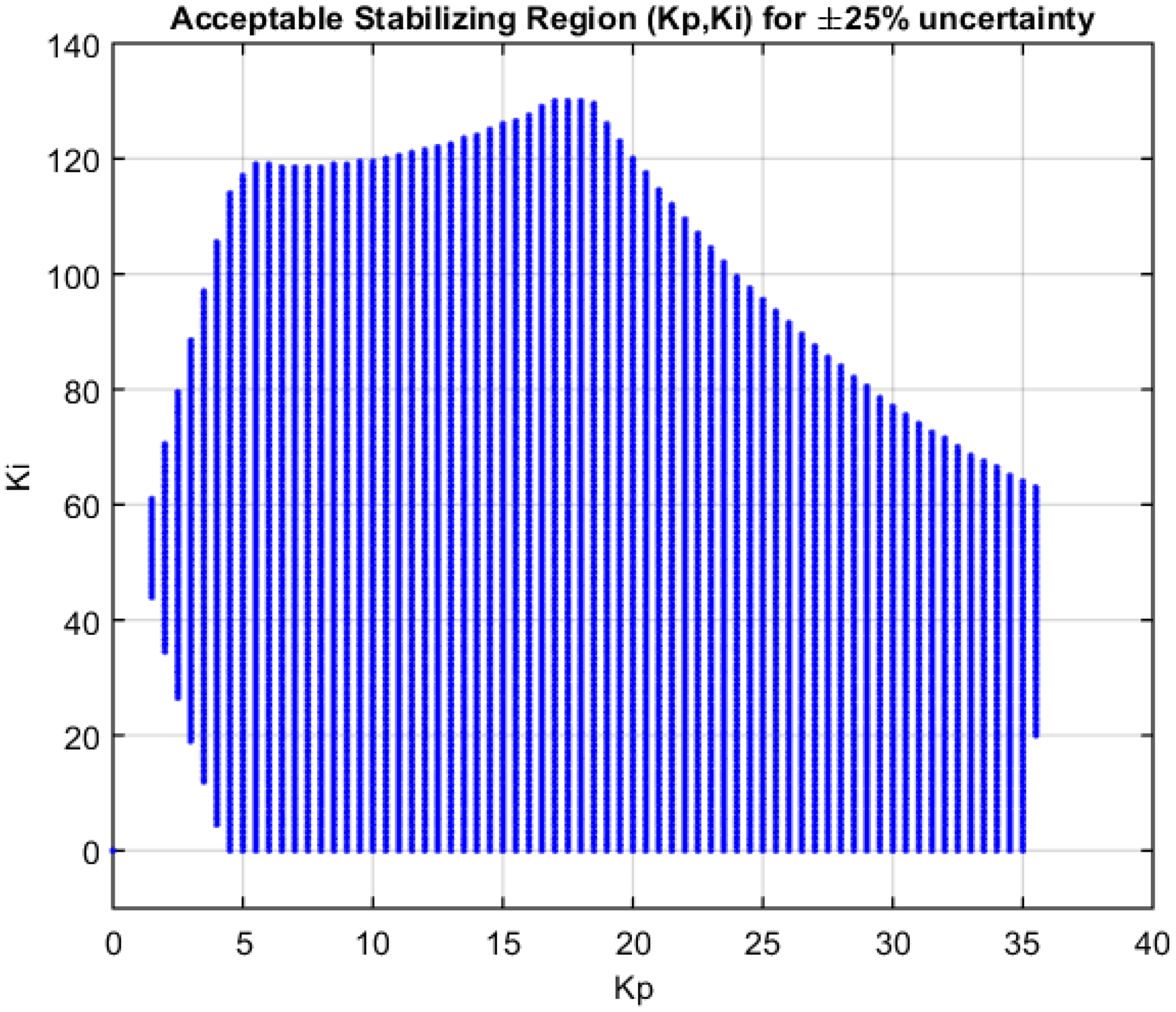
The acceptable stabilizing region for (K_p, K_i) for a ± 25% uncertainty being incorporated into the WT's mathematical model.

Sub-regions of the controllers for each individual plant

A sub-region is taken as the chosen portion from the acceptable stabilizing region presented in 5.2 for each individual plant. The sub-regions for each individual plant are depicted in Figure 4. It falls within the acceptable region for (K_p, K_i). These controllers gain sets can achieve the desired time response specifications, viz., peak overshoot < 5% and settling time < 5 s.

Findings and discussions

After uncertainties were incorporated into the WT's system matrix $\bar{A}$ , 150 iterations of simulations were run to ascertain the lower and upper bounds of both numerator coefficients and denominator coefficients. A seventh-order denominator and a fourth-order numerator were derived. Equation (11) may be used to write the polynomials obtained for the numerator (N₁, N₂, N₃, N₄) and the denominator (D₁, D₂, D₃, D₄). These 8 Kharitonov polynomials are used to construct the 16 required Kharitonov plants. For the 7-state WT, the denominator, D_i(s), and the numerator, N_i(s), where i = 1, 2, 3, 4, have been determined and are shown in detail in Tables 1 and 2. Subsequently, Kharitonov's rectangles are formed to satisfy the zero-exclusion principle (Asadi, 2018) as shown in Figure 2. The robustly stabilizing PI controller is obtained by designing the acceptable region (K_p, K_i) as shown in Section 5.2.

In this paper, the primary aspect in the design of a PI controller (Figure 3) is to robustly stabilize (rotor rated speed, 42 rpm) an uncertain seven-state WT, applied with ±25% uncertainty on 21 elements of its system matrix. To achieve the robustly stabilizing acceptable (K_p, K_i) region shown in Figure 4, which is an intersection of all 16 plants, 150 iterations were executed in the simulations. The (K_p, K_i)-region is shown for all 16 plants collectively (Figure 4) and the sub-regions for all 16 plants individually (Figure 5). It is observed that any point in the 2-dimensional (K_p, K_i) region can robustly stabilize the uncertain WT effectively. But eventually, what matters is the minimization of time response specifications. Hence, the sub-region is extracted from the (K_p, K_i) region based on peak overshoots (<5%) and settling times (<5 s).

Figure 5.

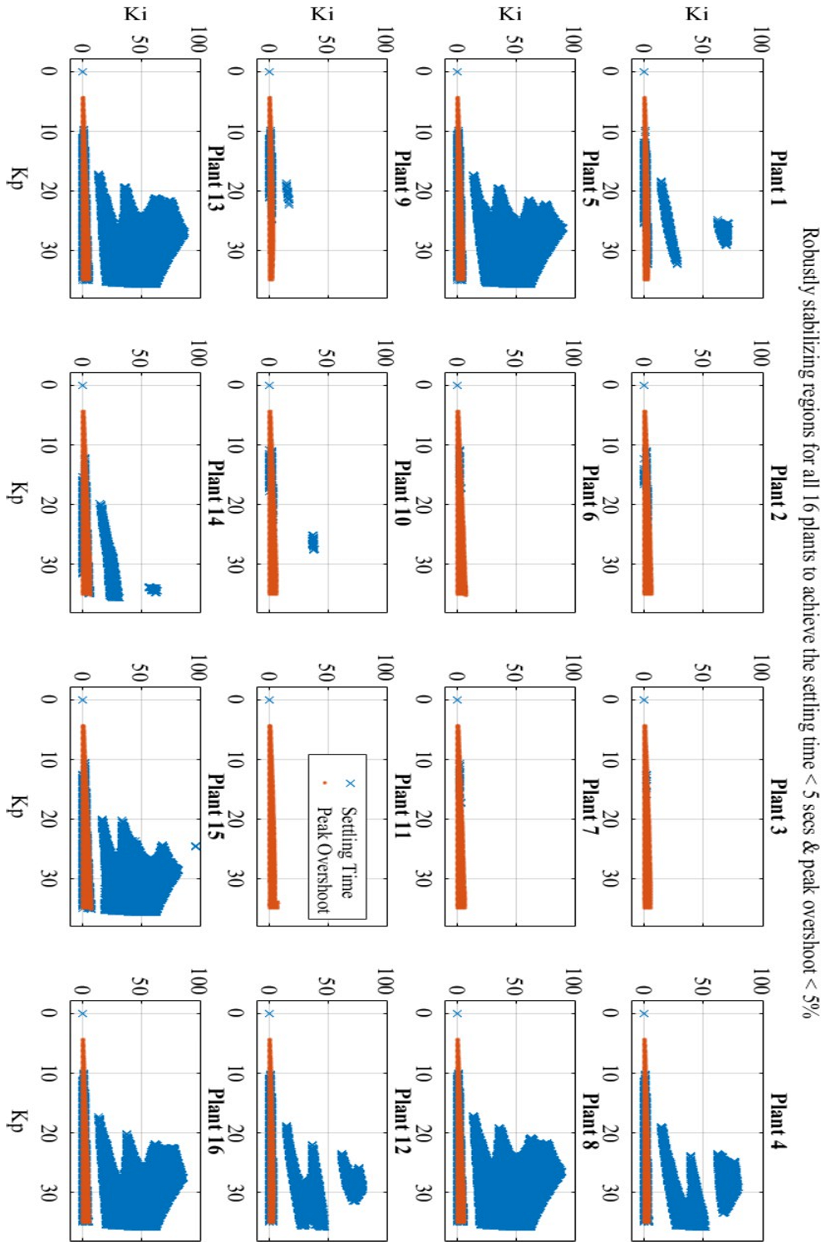
The (K_p, K_i)-subregions for all 16 plants to achieve peak overshoot < 5% and settling time < 5 s.

Settling time and % peak overshoot

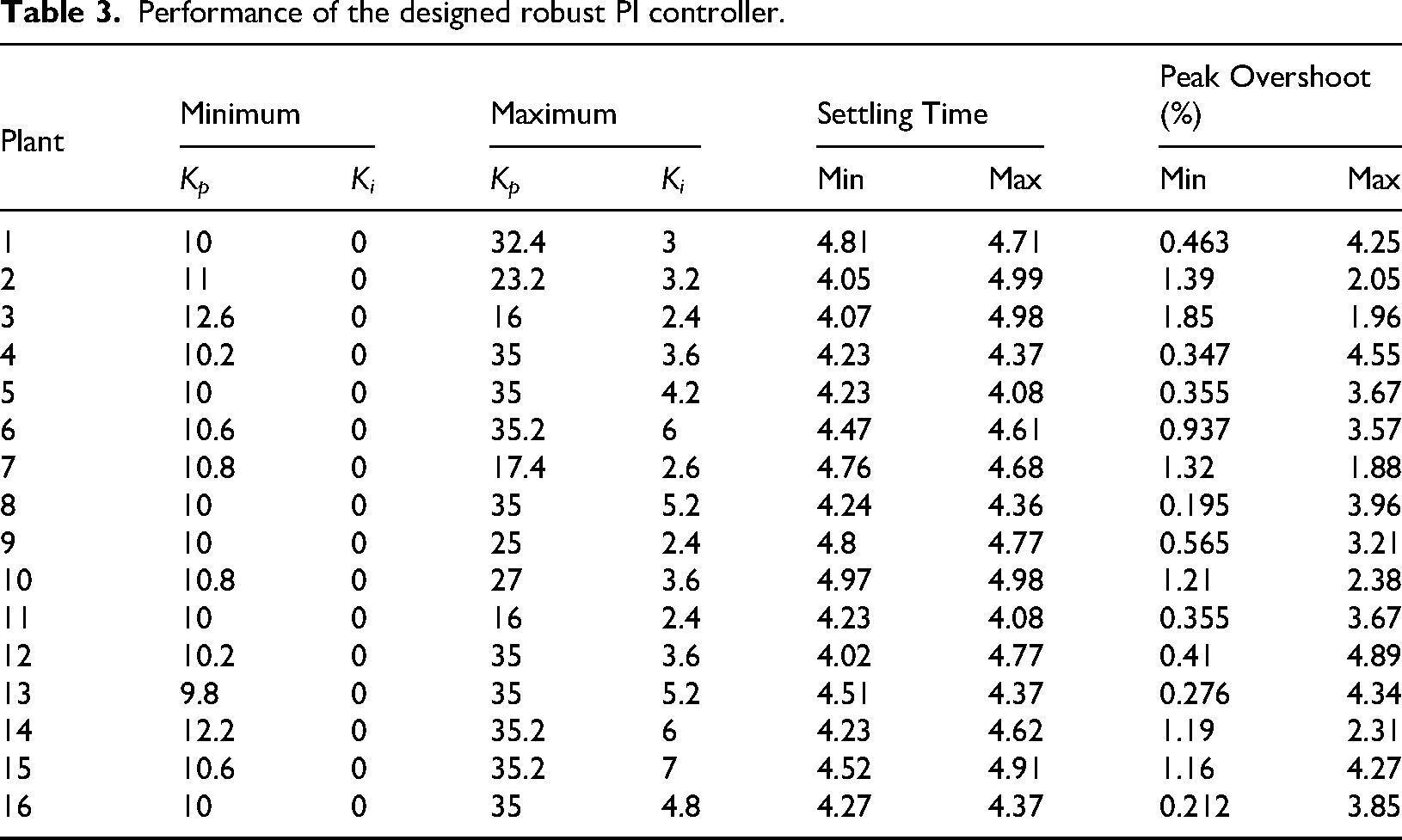
The minimum value and maximum value of both K_p and K_i in each sub-region were extracted and furnished in Table 3, which again presents the settling times and peak overshoot of each Kharitonov plant individually. These time response specifications are in accordance with Figure 6. It is observed that the 12^th Plant controlled by gains (10.2, 0) has a minimum settling time of 4.02 s with a % peak overshoot of 0.41%. Similarly, two of the 16 plants numbered 5 and 11 which are controlled by different gains (35, 4.2) and (16, 2.4) respectively, achieved same settling times (4.08 s minimum) and same % peak overshoot (3.67%) shown in the maximum (K_p, K_i) column of Table 3. The plant numbered 8 could achieve the lowest % peak overshoot (0.195%) that was controlled by gains (10, 0). Similarly, the plant numbered 12 has the maximum % peak overshoot (4.89%) that was controlled by gains (35, 3.6).

Figure 6.

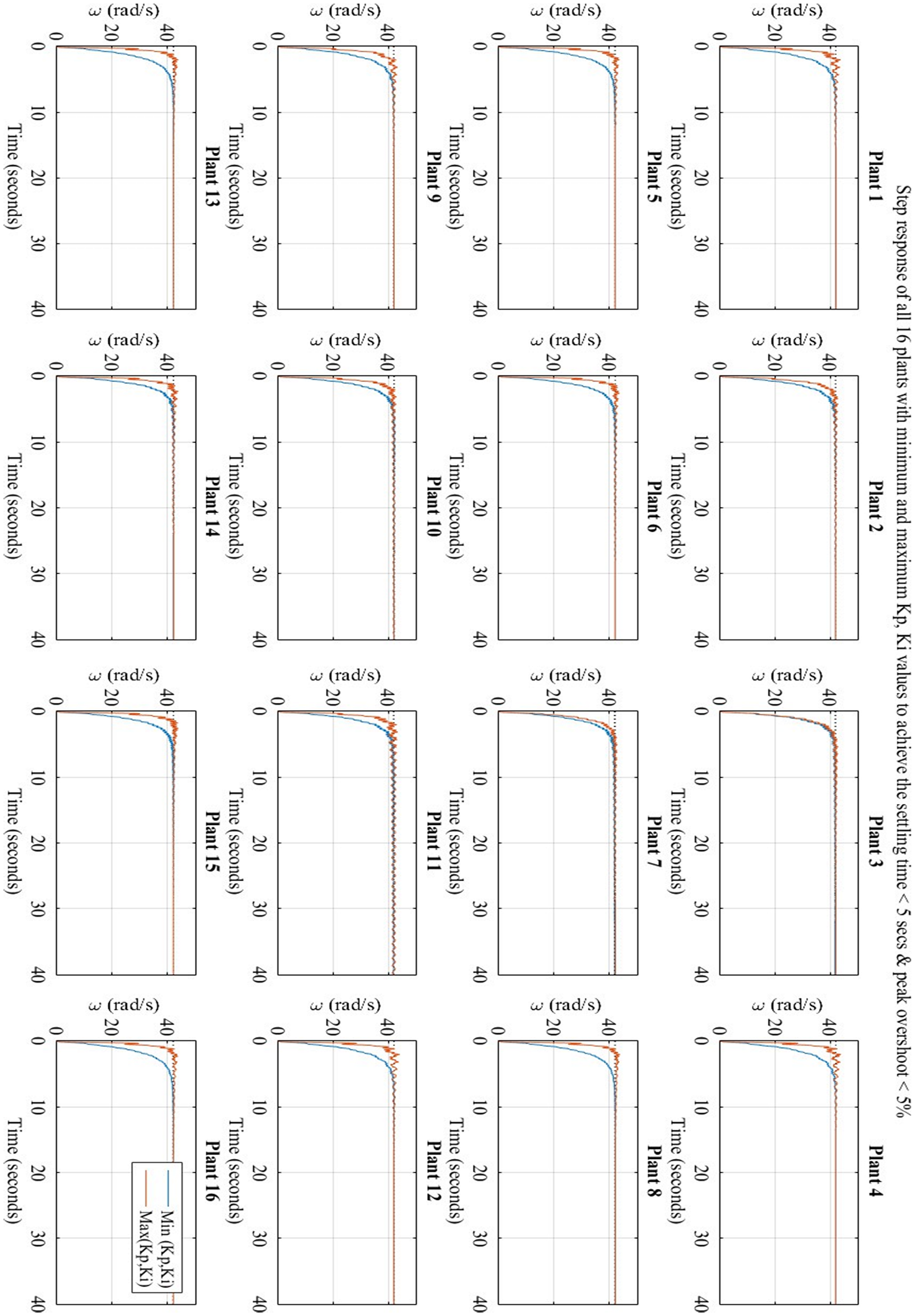
The step response of all 16 plants with the lowest and highest K_p, K_i values to get the appropriate peak overshoot and settling time.

Table 3.

Performance of the designed robust PI controller.

Plant	Minimum		Maximum		Settling Time		Peak Overshoot (%)
	K_p	K_i	K_p	K_i	Min	Max	Min	Max
1	10	0	32.4	3	4.81	4.71	0.463	4.25
2	11	0	23.2	3.2	4.05	4.99	1.39	2.05
3	12.6	0	16	2.4	4.07	4.98	1.85	1.96
4	10.2	0	35	3.6	4.23	4.37	0.347	4.55
5	10	0	35	4.2	4.23	4.08	0.355	3.67
6	10.6	0	35.2	6	4.47	4.61	0.937	3.57
7	10.8	0	17.4	2.6	4.76	4.68	1.32	1.88
8	10	0	35	5.2	4.24	4.36	0.195	3.96
9	10	0	25	2.4	4.8	4.77	0.565	3.21
10	10.8	0	27	3.6	4.97	4.98	1.21	2.38
11	10	0	16	2.4	4.23	4.08	0.355	3.67
12	10.2	0	35	3.6	4.02	4.77	0.41	4.89
13	9.8	0	35	5.2	4.51	4.37	0.276	4.34
14	12.2	0	35.2	6	4.23	4.62	1.19	2.31
15	10.6	0	35.2	7	4.52	4.91	1.16	4.27
16	10	0	35	4.8	4.27	4.37	0.212	3.85

Real-time simulations of robust controllers for the 16-plant model of an uncertain wind turbine

This paper also presents real-time simulation results of the designed robust controllers for an uncertain multi-input wind turbine. The real-time simulation set-up is shown in Figure 7. The real-time simulation software is completely compatible with the MATLAB/SIMULINK environment (Mohanty et al., 2018). The Simulink model is built, loaded, and executed by the real-time simulation software in the OPAL RT OP5700 Simulator. The rotor speed of 42 rpm is obtained for all 16 plants formed in section 4.1 in a real-time environment. The same two sets (minimum and maximum combinations given in Table 3) of controller gains were used to check for the robustness of the designed controllers in a real-time environment. Results of all 16 plants are shown in Figure 8, where it is observed that the desired specifications, namely, the settling times less than 5 s and peak overshoots less than 5%, are achieved, which validates the performance of all designed controllers in MATLAB shown in Figure 6.

Figure 7.

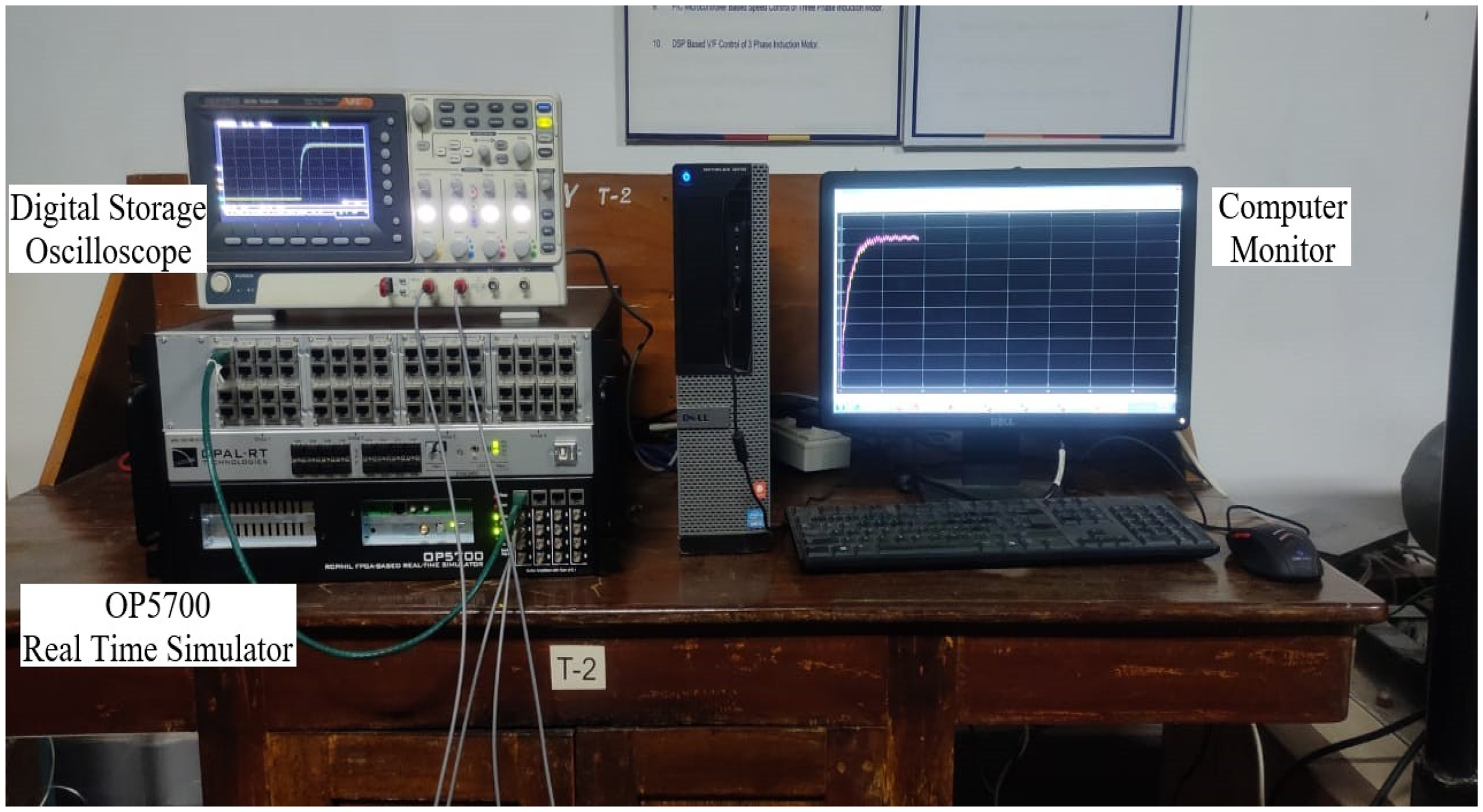
Set-up of real-time simulation.

Figure 8.

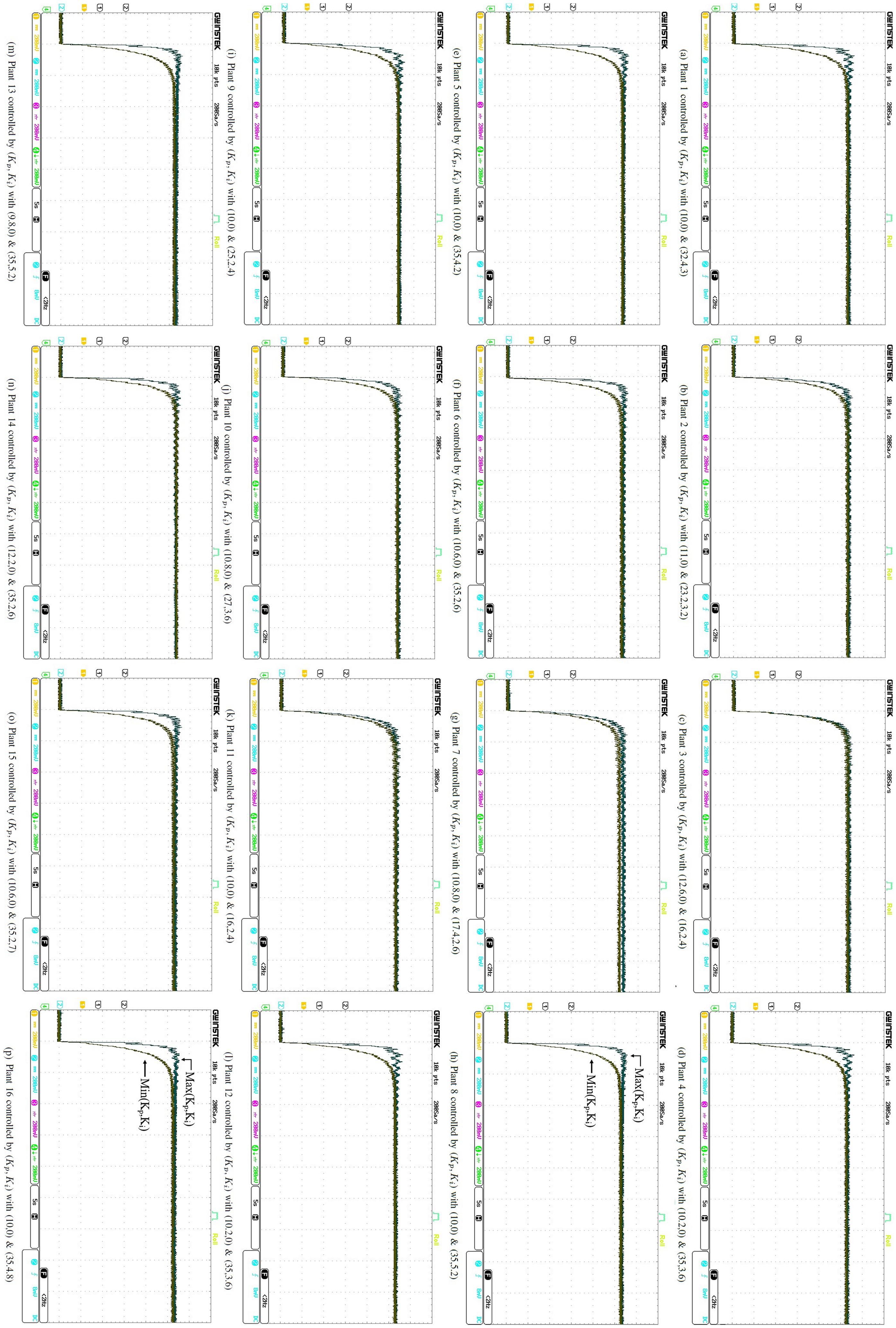
The real-time simulation results for controlling the rotor speed to 42 rpm rated value. Plants numbered 1 to 16 are shown in this figure.

Conclusion

A multi-input WT with control input(β) and wind disturbances is considered and subjected to ±25% uncertainty. The system matrix has twenty-one elements to which this uncertainty value is applied. Kharitonov's 16-plant theorem approach is used to design the robustly stabilizing (K_p, K_i) region by forming Kharitonov's rectangles. In this case, any value of K_p & K_i in this area may robustly stabilize the wind turbine, i.e., regulate the rotor speed to its rated value of 42 rpm. A sub-region is also formed for all the 16 plants individually to solely achieve the desired time response specifications, which are settling times less than 5 s and peak overshoots less than 5%. Eventually, the minimum and maximum values of (K_p, K_i) chosen from the sub-regions are found to strictly achieve the mentioned specifications, which validates the performance of robust controllers designed in MATLAB. To further evaluate the ad, validate the performances, real-time simulations made on the OPAL RT OP5700 simulator are also furnished.

Footnotes

ORCID iDs

Daniel Eutyche Mbadjoun Wapet

Mohamed Metwally Mahmoud

Authorship contribution

All authors have equally contributed to every facet of this research. Their joint efforts encompassed: Conceptualization; Data curation; Formal analysis; Investigation; Methodology; Project administration; Resources; Software; Supervision; Validation; Visualization; Roles/Writing—original draft; and Writing—review and editing.

Funding

The authors received no financial support for the research, authorship, and/or publication of this article.

Declaration of conflicting interests

The authors declared no potential conflicts of interest with respect to the research, authorship, and/or publication of this article.

Data availability statement

Availability of data and materials Datasets used and/or analyzed during the current study are available from the corresponding author upon reasonable request.

References

Adeoye

Binzaid

Attia

(2024) Performance of an omnidirectional wind energy harvesting system for low wind-speeds. In: 2024.

Aldin

NAN

Abdellatif

WSE

Elbarbary

ZMS

, et al. (2023) Robust speed controller for PMSG wind system based on harris hawks optimization via wind speed estimation: A real case study. IEEE Access 11: 5229–5943.

Apata

Oyedokun

DTO

(2020) An overview of control techniques for wind turbine systems. Scientific African 10: e00566.

Asadi

(2018) Robust control of DC-DC converters: The Kharitonov’s theorem approach with MATLAB® codes. Synthesis Lectures on Power Electronics. https://link.springer.com/book/10.1007/978-3-031-02503-7

Atia

Mahmoud

Elzein

, et al. (2024) Applications of Kepler algorithm-based controller for DC chopper: Towards stabilizing wind driven PMSGs under nonstandard voltages. Sustainability (Switzerland) 16(7): 2952–2977.

Bahmani

Bayat

Golchin

(2020) Wind turbines power regulation using a low-complexity linear parameter varying-model predictive control approach. Transactions of the Institute of Measurement and Control 42(1): 81–93.

Bhattacharyya

(2017) Robust control under parametric uncertainty: An overview and recent results. Annual Reviews in Control 44: 45–77.

Boudjemai

Ahmed

Mehdi

, et al. (2023a) Experimental analysis of a new low power wind turbine emulator using a DC machine and advanced method for Maximum wind power capture. IEEE Access 11: 92225–92241.

Boudjemai

Ardjoun

Chafouk

, et al. (2023b) Application of a novel synergetic control for optimal power extraction of a small-scale wind generation system with variable loads and wind speeds. Symmetry 15(2): 92225–92241.

10.

Boudjemai

Ardjoun

SAEM

Chafouk

, et al. (2025) Design, simulation, and experimental validation of a new fuzzy logic-based maximal power point tracking strategy for low power wind turbines. International Journal of Fuzzy Systems 5(1): 296–310.

11.

Boutabba

Benlaloui

Mechnane

, et al. (2025) Design of a small wind turbine emulator for testing power converters using dSPACE 1104. International Journal of Robotics and Control Systems 5(2): 698–712.

12.

Cascianelli

Astolfi

Castellani

, et al. (2022) Wind turbine power curve monitoring based on environmental and operational data. IEEE Transactions on Industrial Informatics 18(8): 5209–5218.

13.

Chishti

Murshid

Singh

(2020) Robust normalized mixed-norm adaptive control scheme for PQ improvement at PCC of a remotely located wind-solar PV-BES microgrid. IEEE Transactions on Industrial Informatics 16(3): 1708–1721.

14.

Chu

(2018) Graphical robust PID tuning based on uncertain systems for disturbance rejection satisfying multiple objectives. International Journal of Control, Automation and Systems 16(5): 2033–2042.

15.

El Beshbichi

Xing

Chen Ong

(2023) Modelica-AeroDyn: Development, benchmark, and application of a comprehensive object-oriented tool for dynamic analysis of non-conventional horizontal-axis floating wind turbines. Wind Energy 26(6): 538–572.

16.

Errouissi

Al-Durra

Debouza

(2018) A novel design of PI current controller for PMSG-based wind turbine considering transient performance specifications and control saturation. IEEE Transactions on Industrial Electronics 65(11): 8624–8634.

17.

Fayz

Ahmed

Elzein

, et al. (2025) Optimal controller design of crowbar system for DFIG-based WT : Applications of gravitational search algorithm. Buletin Ilmiah Sarjana Teknik Elektro 7(2): 122–136.

18.

Habibi

Rahimi Nohooji

Howard

(2018) Adaptive PID control of wind turbines for power regulation with unknown control direction and actuator faults. IEEE Access 6: 37464–37479.

19.

Hamoodi

Hameed

Hamoodi

(2020) Pitch angle control of wind turbine using adaptive fuzzy-PID controller. EAI Endorsed Transactions on Energy Web 7(28): e15.

20.

Huang

Chen

Liang

, et al. (2020) Prediction of salt contamination in the rotating blade of wind turbine under lightning strike occurrence using fuzzy c-means and kmeans clustering approaches. IET Science, Measurement and Technology 14(1): 91–97.

21.

Isbeih

El Moursi

Xiao

, et al. (2019) H∞ mixed-sensitivity robust control design for damping low-frequency oscillations with DFIG wind power generation. IET Generation, Transmission and Distribution 13(19): 4274–4286.

22.

Jafari

Shahgholian

(2017) Analysis and simulation of a sliding mode controller for mechanical part of a doubly-fed induction generator-based wind turbine. IET Generation, Transmission and Distribution 11(10): 2677–2688.

23.

Kheshti

Ding

Bao

, et al. (2020) Toward intelligent inertial frequency participation of wind farms for the grid frequency control. IEEE Transactions on Industrial Informatics 16(11): 6772–6786.

24.

Liu

Han

Wang

(2017) Second-order sliding mode control for power optimisation of DFIG-based variable speed wind turbine. IET Renewable Power Generation 11(2): 408–418.

25.

Mahmoud

Atia

Abdelaziz

, et al. (2022a) Dynamic performance assessment of PMSG and DFIG-based WECS with the support of manta ray foraging optimizer considering MPPT, pitch control, and FRT capability issues. Processes 10(12): 2723–2751.

26.

Mahmoud

Atia

Esmail

, et al. (2023a) Evaluation and comparison of different methods for improving fault ride-through capability in grid-tied permanent magnet synchronous wind generators. International Transactions on Electrical Energy Systems 2023: 1–22.

27.

Mahmoud

Khalid Ratib

Aly

, et al. (2022b) Wind-driven permanent magnet synchronous generators connected to a power grid: Existing perspective and future aspects. Wind Engineering 46(1): 189–199.

28.

Mahmoud

Salama

Bajaj

, et al. (2023b) Integration of wind systems with SVC and STATCOM during Various events to achieve FRT capability and voltage stability: Towards the reliability of modern power systems. International Journal of Energy Research 2023: 1–28.

29.

Matušů

(2011) Calculation of all stabilizing PI and PID controllers. International Journal of Mathematics and Computers in Simulation 5(3): 224–231.

30.

Menzri

Boutabba

Benlaloui

, et al. (2024) Applications of novel combined controllers for optimizing grid-connected hybrid renewable energy systems. Sustainability (Switzerland) 16(16): 6825–6849.

31.

Metwally Mahmoud

(2023) Improved current control loops in wind side converter with the support of wild horse optimizer for enhancing the dynamic performance of PMSG-based wind generation system. International Journal of Modelling and Simulation 43(6): 952–966.

32.

Mohanty

Viswavandya

Ray

, et al. (2018) Literature survey on OPAL-RT technologies with advance features and Industrial applications. In: 1st International Conference on Advanced Research in Engineering Sciences, ARES 2018, 2018.

33.

Naghdalian

Amraee

Kamali

, et al. (2020) Stochastic network-constrained unit commitment to determine flexible ramp reserve for handling wind power and demand uncertainties. IEEE Transactions on Industrial Informatics 16(7): 4580–4591.

34.

Petkov

Slavov

Kralev

(2018) Design of Embedded Robust Control Systems Using MATLAB®/Simulink® .

35.

Rigatos

Siano

(2011) Design of robust electric power system stabilizers using Kharitonov’s theorem. Mathematics and Computers in Simulation 82(1): 181–191.

36.

Saidi

Mezouar

Miloud

, et al. (2021) Adaptive control of wind turbine generators for power capture optimization by using integral backstepping approach during partial-load operation. Journal of Control, Automation and Electrical Systems 32(4): 1041–1052.

37.

Salem

Abu-Siada

Islam

(2017) Improved condition monitoring technique for wind turbine gearbox and shaft stress detection. IET Science, Measurement and Technology 11(4): 431–437.

38.

Soliman

Hasanien

Azazi

, et al. (2019) An adaptive fuzzy logic control strategy for performance enhancement of a grid-connected PMSG-based wind turbine. IEEE Transactions on Industrial Informatics 15(6): 3163–3173.

39.

Toulabi

Dobakhshari

Ranjbar

(2018) Optimal robust first-order frequency controller design for DFIG-based wind farm utilising 16-plant theorem. IET Renewable Power Generation 12(3): 298–310.

40.

(2018) Fast stability analysis for proportional-integral controller in interval systems. Journal of Advanced Engineering and Computation 2(2): 111.

41.

Wang

Gao

, et al. (2018) Robust model reference adaptive control design for wind turbine speed regulation simulated by using FAST. Journal of Energy Engineering 144(2): 04018007.

42.

Wright

Balas

(2003) Design of state-space-based control algorithms for wind turbine speed regulation. Journal of Solar Energy Engineering, Transactions of the ASME 125(4): 386–395.

Design and real-time simulations of robust controllers for uncertain multi-input wind turbine

Abstract

Keywords

Introduction

WT mathematical model

The uncertain WT model

Kharitonov's theorem preliminaries

Formation of 16 Kharitonov plants

Kharitonov's rectangles

The robust controller design methodology utilizing a 16-plant model

Procedure for designing suitable gains for the controller

Acceptable stabilizing region of the controller

Sub-regions of the controllers for each individual plant

Findings and discussions

Settling time and % peak overshoot

Real-time simulations of robust controllers for the 16-plant model of an uncertain wind turbine

Conclusion

Footnotes

ORCID iDs

Authorship contribution

Funding

Declaration of conflicting interests

Data availability statement

References