Sage Journals: Discover world-class research

Abstract

Accurate prediction of biochar yield from biomass pyrolysis is essential for optimizing production in sustainable agriculture, yet remains technically challenging due to multiple interacting factors. This study developed a predictive framework using a curated dataset of 211 samples, each including 14 normalized input features (chemical, physical, operational) and one output variable (biochar yield, wt%). Machine learning modeling utilized Gradient Boosted Decision Trees (GBDT), with hyperparameters exhaustively tuned via Gaussian Processes Optimization (GPO), Evolutionary Strategies (ES), Bayesian Probability Improvement (BPI), and Batch Bayesian Optimization (BBO). Models were evaluated on a train-test split (90% training, 10% testing) and the best performance was achieved by the GBDT–BPI model: total R² = 0.982, mean squared error (MSE) = 1.65, average absolute relative error percentage (AARE%) = 1.35; on the test set, R² = 0.693, MSE = 15.2, AARE% = 9.54. Comparative analysis showed GBDT–BPI outperformed GBDT–GPO (total R² = 0.978; MSE = 2.01; AARE% = 1.72), GBDT–ES (total R² = 0.976; MSE =  2.13; AARE% = 3.81), and GBDT–BBO (total R² = 0.980; MSE = 1.81; AARE% = 2.58). Sensitivity study presented reside duration, temperature, and fixed carbon as the top parameters of yield. Time efficiency was comparable for all optimizers, with BBO taking the longest (313 s/500 iterations). Diagnostic leverage analysis demonstrated high data quality, with less than 1% flagged as influential outliers. This integrated approach delivered high-accuracy, interpretable prediction, and revealed critical parameters for process optimization in biomass pyrolysis workflows.

Keywords

Biochar yield biomass pyrolysis machine learning GBDT optimization feature importance

Introduction

Biomass refers to all forms of organic material generated by living organisms and is considered among the most plentiful natural resources on the planet, with global yearly production reaching nearly 105 billion metric tons of carbon (Heinimö and Junginger, 2009; Jenkins, 2015). Of this total, terrestrial environments contribute about half, while the remainder arises from marine sources, such as algae. Biomass encompasses a broad array of origins, including wood and forest residues, crop byproducts like sugarcane bagasse, rice straw, wheat straw, and even urban solid waste. Historically, humans have relied on biomass for both energy generation and the production of various materials over thousands of years (Börjesson, 1996; Garcia et al., 2019; Wullschleger et al., 2010).

Currently, around 80% of the world's energy requirements are satisfied by fossil fuels, which has led to pressing environmental issues (Khezerloo-ye Aghdam et al., 2023 , 2024 , 2019). The consumption of finite resources such as coal, oil, and natural gas is linked to serious impacts including greenhouse gas emissions, air quality deterioration, and climate change. Notably, coal still supplies close to one-third of the world's energy, and its continued use is projected to quadruple global carbon emissions by 2030 if trends persist. In response to these concerns, renewable energy solutions are becoming increasingly vital. Among such alternatives, energy derived from biomass is particularly notable due to its renewability, availability, and sustainability (Vassilev et al., 2013, 2015). Compared to conventional fossil sources, biomass is advantageous as it can minimize net carbon emissions through the replanting of crops, supporting both environmental protection and energy resilience (Canam et al., 2013; Yang et al., 2019a).

Although biomass holds significant potential, its direct use is hindered by several issues such as low grindability, elevated moisture content, low energy density, and the tendency to cause fouling and slagging from ash during combustion (Fransen and De Kroon, 2001; Vassilev et al., 2015). These challenges make it necessary to preprocess biomass to enhance its suitability for energy production. One popular solution is pyrolysis—a thermochemical conversion process that transforms raw biomass into more manageable and efficient energy forms. During pyrolysis, biomass is heated in the absence of oxygen at moderate temperatures (typically 350–650 °C), generating three distinct products: bio-oil (liquid), syngas (gas), and biochar. Recently, biochar has drawn considerable interest because of its versatile roles on agricultures, energy, and environmental management (Li et al., 2023; Selvarajoo et al., 2022; Yoder et al., 2011).

Biochar, which is rich in carbon and produced through pyrolysis, serves many functions due to its unique properties. It is especially valued for enhancing soil fertility, improving water retention, and acting as a means to sequester carbon, all of which contribute to alleviating climate change (Yang et al., 2019b; Zhu et al., 2022). In addition to its agricultural applications, biochar is effective in environmental management, as it can absorb pollutants and serve as a precursor to value-added materials like activated carbon. Compared to untreated biomass, biochar offers higher carbon content, greater energy density, and superior heating value, making it more effective as a solid fuel (Brown et al., 2011; Laird et al., 2009). Historically, both biochar and charcoal were essential resources for various uses including energy and industry. Modern research has expanded the use of biochar in farming systems and is actively investigating its potential in environmental remediation, highlighting the importance of optimizing the processes used to produce it (Jha et al., 2010; Schmidt et al., 2021).

The quality and efficiency of biochar production are influenced by numerous variables, most notably the conditions under which pyrolysis occurs and the specific type of biomass used as input (Jahan et al., 2024; Wang et al., 2025). Key operational settings directly affect both the yield and properties of the resulting biochar. Research consistently finds that lower pyrolysis temperatures (typically 300–450°C) tend to deliver higher yields, while applying higher temperatures increases the release of volatile substances, thus lowering yield but making the biochar more aromatic and chemically stable (Mašek et al., 2013; Tomczyk et al., 2020). Likewise, extending the residence time promotes more thorough carbonization, resulting in biochar with a higher fixed carbon content. Other aspects like operating pressure and the nature of the surrounding gas during pyrolysis also have significant roles. While nitrogen is commonly used to create an oxygen-free environment and prevent unwanted reactions, recent findings suggest that using CO₂ recovered from flue gases can reduce costs without negatively impacting carbon sequestration properties in the final product (Ronsse et al., 2013; Yu et al., 2018).

The makeup of the biomass feedstock itself also greatly affects both how much biochar is produced and its final characteristics. Biomass consists mainly of cellulose, hemicellulose, and lignin—each following unique degradation patterns during pyrolysis, which in turn explains the differences in biochar quantity and quality between various feedstocks. For instance, cellulose starts degrading at 200–300 °C, primarily forming bio-oil precursors like levoglucosan and other aliphatic substances; hemicellulose breaks down to yield products such as furans. Lignin decomposes over a wider temperature window and mainly contributes to forming aromatic structures, making biochar produced from lignin-rich feedstocks more stable and carbon-dense. Since every type of biomass reacts differently during pyrolysis, understanding these specifics is crucial for optimizing biochar performance (Elkhalifa et al., 2019; Tripathi et al., 2016; Zhu et al., 2022)

Beyond energy production, biochar proves especially valuable in agriculture. It helps improve soil structure, strengthen nutrient retention, and reduce reliance on synthetic fertilizers—all vital for sustainable agriculture and climate resilience (Allohverdi et al., 2021; Jha et al., 2010). Its ability to lock away carbon makes it an important tool in global carbon management strategies. Ongoing studies are examining how varying the pyrolysis process, choice of biomass, and resulting biochar properties impact its effectiveness in different applications. For persistent carbon storage, for example, biochars with higher fixed carbon content and suitable H:C and O:C atomic ratios are considered more robust and stable for long-term sequestration.

Given the pressing need for accurate prediction and optimization of biochar yield in sustainable energy and agricultural contexts, this research holds substantial practical significance. By systematically applying advanced machine learning and optimization strategies to a unique and rigorously curated dataset, this study addresses the longstanding challenge of reliably forecasting biochar output from diverse biomass sources. The research (work flow presented in Figure 1) hypothesizes that integrating multiple machine learning models, combined with state-of-the-art hyperparameter optimization (Gaussian Processes Optimization (GPO), Evolutionary Strategies (ES), Bayesian Probability Improvement (BPI), and Batch Bayesian Optimization (BBO)), will lead to significant improvements in prediction accuracy. The workflow encompasses data normalization, model selection, sensitivity and feature importance analysis (using both correlation matrices and SHapley Additive exPlanations (SHAP) values), and comparative evaluation of four optimization approaches on Gradient Boosted Decision Trees (GBDT) performance. The main objectives are to identify the most influential features affecting biochar yield, benchmark and select the best predictive model, and provide actionable insights for future experimental and industrial biochar production.

Figure 1.

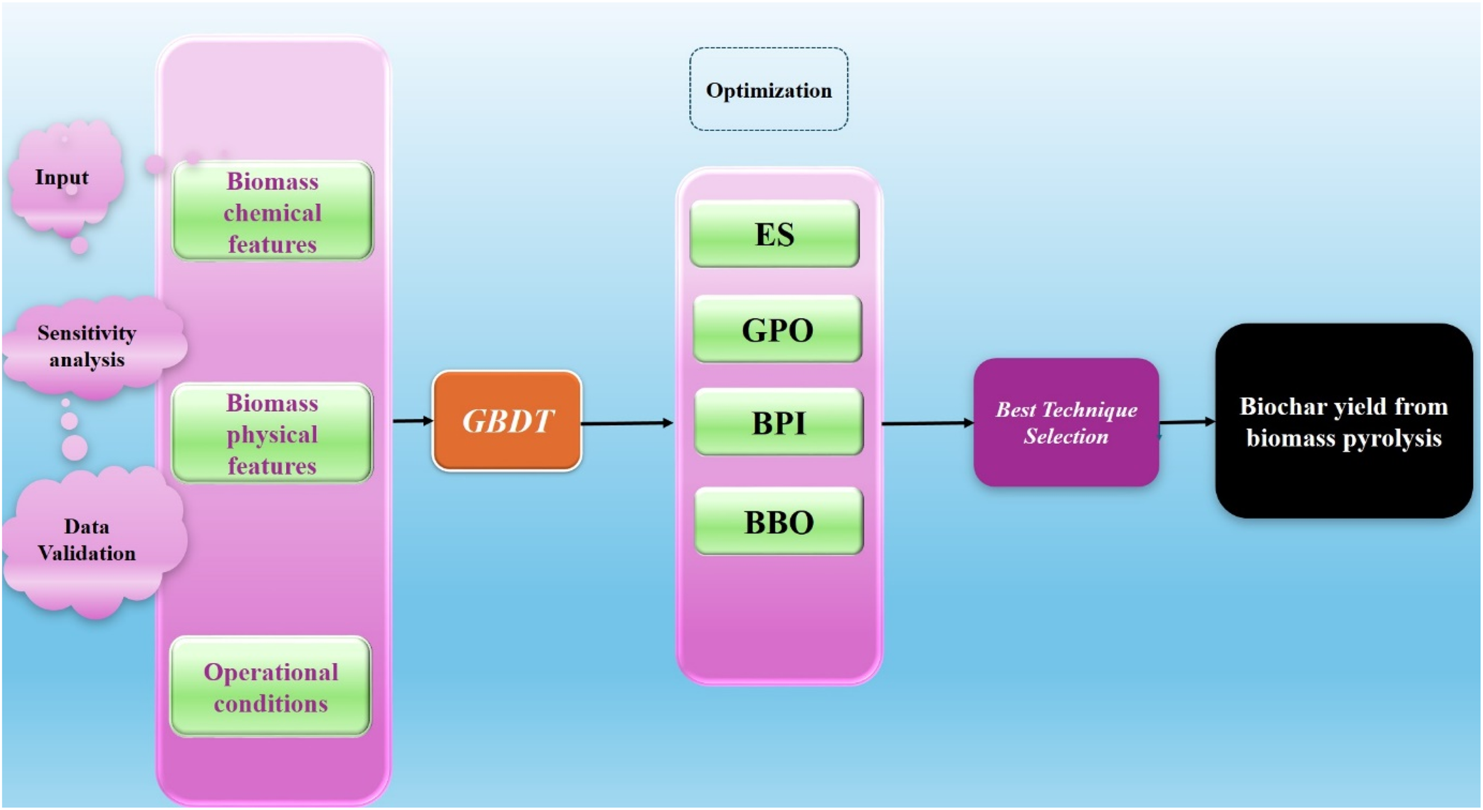
Model construction workflow utilized in this study.

Methodology

Analysis of the collected database

The dataset utilized in this research to develop and validate the predictive model originated from a comprehensive review of academic literature related to biochar production, with an emphasis on biomass pyrolysis studies (Chaihad et al., 2021; Gurevich Messina et al., 2017; Hatefirad et al., 2022; Li et al., 2022b; Mishra and Mohanty, 2022; Ozbay et al., 2019; Park et al., 2020; Shahsavari and Sadrameli, 2020; Shen and Chen, 2023; Wei et al., 2020 , 2022; Wu et al., 2022a, 2022b; Xue et al., 2022; Yang et al., 2020; Yarbay Şahin and Özbay, 2021; Zeng et al., 2021; Zhang et al., 2015 , 2017). Sources were carefully chosen from leading, high-impact journals within the discipline to ensure the reliability and integrity of the compiled data. In total, the dataset includes 14 distinct input features alongside a single target variable, which serves as the basis for prediction using a variety of machine learning algorithms.

These input features are organized into three main categories. The first group pertains to the chemical and compositional properties of the biomass feedstock, capturing values for carbon, hydrogen, nitrogen, oxygen, ash content, fixed carbon, volatile matter (all as percentages), and catalyst acid site content (measured in mmol/g). The second category addresses physical attributes, specifically the crystallinity index and BET surface area of the biomass. The final group relates to operational conditions, comprising catalyst-to-biomass ratio, pyrolysis temperature (in °C), and residence time (in minutes).

The variable targeted for prediction is biochar yield, recorded as the weight percentage (wt%) of the total products produced during the pyrolysis process. While pyrolysis results in an array of outputs such as syngas, alcohols, and other compounds, biochar yield is particularly noteworthy due to its relevance to agricultural enhancement and food production.

This dataset encompasses 211 individual samples. For the purposes of model development, 90% of the entries were designated for training, with the remaining 10% held back to evaluate model performance. The distribution and value ranges for both the inputs and the output variable are illustrated in Figure 2 by means of boxplots.

Figure 2.

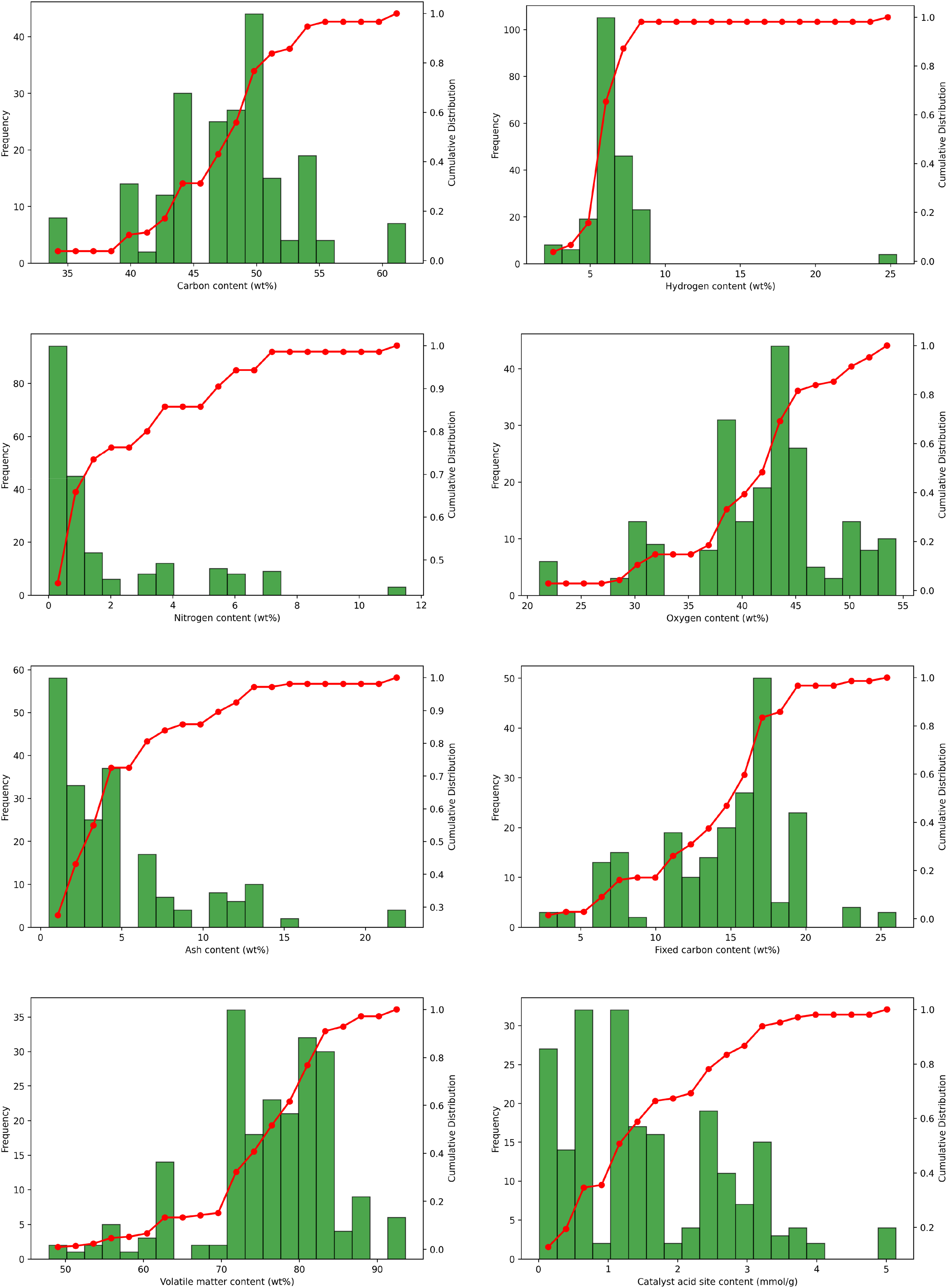
Boxplots illustrating the statistical distribution and range of all input and output variables in the dataset.

Gradient boosting decision tree

GBDT is an ensemble machine learning algorithm that builds predictive models by combining multiple weak learners, typically decision trees, in a sequential manner. The main idea behind gradient boosting is to iteratively improve model performance by focusing on the errors of previous models—each new tree attempts to correct the mistakes made by the ensemble so far. GBDT is widely used in both regression and classification tasks because of its high predictive accuracy and flexibility.

Mathematically, GBDT works by optimizing a loss function through gradient descent in function space. At each iteration, the algorithm computes the negative gradient (the residual errors of the current prediction), which represents the direction of steepest descent, and fits a new decision tree to these residuals. The model's prediction is updated by adding this new tree, weighted by a learning rate parameter. This process is repeated for a specified number of iterations or until the error stops improving, resulting in a strong predictive model composed of many weak trees.

GBDT is popular in practical applications such as credit scoring, forecasting, ranking tasks, and risk assessment due to its ability to handle different types of data and capture complex nonlinear relationships. Its advantages include robustness to overfitting (especially with proper regularization), support for various loss functions, and automatic feature selection. Modern implementations like XGBoost, LightGBM, and CatBoost offer further enhancements in speed and scalability, making gradient boosting a top choice for structured data problems.

Optimization algorithms

Gaussian process optimization

GPO, often called Bayesian Optimization with Gaussian Processes, is a probabilistic, model-based approach used for optimizing expensive or black-box functions. The core idea is to treat the unknown function as a random process and use a Gaussian Process (GP) to model the function's behavior based on observed data points. This approach not only provides a prediction of the function's value at untested points but also quantifies the uncertainty of those predictions, allowing for efficient and informed exploration of the search space.

Mathematically, a GP defines a distribution over possible functions and uses Bayes’ theorem to update this distribution as new data is collected. The GP is characterized by a mean function and a covariance (kernel) function, which encodes assumptions about the function's smoothness and other properties. At each iteration, an acquisition function—such as Expected Improvement (EI) or Upper Confidence Bound (UCB)—is used to select the next point to evaluate by balancing exploitation (testing likely optimal areas) and exploration (sampling uncertain regions). The outcome updates the GP model, gradually zeroing in on the optimal solution with minimal function evaluations.

GPO is particularly advantageous for applications where function evaluations are costly or time-consuming, such as hyperparameter tuning of machine learning models, experimental design, and robotics. Its strengths include efficient use of limited data, the ability to work with noisy observations, and providing uncertainty estimates, which help avoid suboptimal local minima. This makes GPO a go-to choice for black-box optimization tasks with expensive evaluations.

Evolutionary strategies

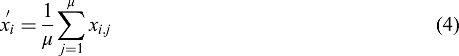
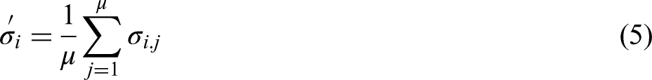
ESs are optimization techniques inspired by the principles of natural evolution, particularly suited for tackling continuous optimization challenges. These algorithms work by evolving a population of candidate solutions over successive generations, utilizing key evolutionary operators such as mutation, recombination, and selection. In ES, each candidate is characterized by a solution vector xxx and an associated vector of strategy parameters σ\sigmaσ, which dictate the mutation strength for each dimension of x (Hansen et al., 2015).

The ES process starts with the initialization of a population of μ\mu μ individuals. Solution vectors x x x are randomly generated within problem-specific bounds [x_i^min,x_i^max], and strategy parameters σ \sigma σ are set within a positive range [σ^min, σ^max]:

x_{i} \sim Uniform (x_{i}^{min}, x_{i}^{max}), σ_{i} \sim Uniform (σ_{i}^{min}, σ_{i}^{max})

(1)

In each generation, λ offspring are created, primarily using mutation, which alters both the solution vectors and their strategy parameters. The updated strategy parameters for each offspring are computed as:

\overset{'}{σ_{i}} = σ_{i} \times \exp (τ \times N (0.1) + \overset{'}{τ} \times N_{i} (0.1))

(2 )

Here N(0.1) is a standard normal random variable and N_i(0.1) is sampled independently for each dimension. The learning rates τ and τ′ are chosen based on dimensionality. With the new strategy parameter, the mutated offspring solution vector is then generated as: (Beyer and Schwefel, 2002):

\overset{'}{x_{i}} = x_{i} + \overset{'}{σ_{i}} N_{i} (0.1)

(3 )

If recombination is employed, information from multiple parents is merged. For intermediate recombination, new solution and strategy parameters are computed as the weighted average across μ\mu μ parents:

\overset{'}{x_{i}} = \frac{1}{μ} \sum_{j = 1}^{μ} x_{i . j}

(4 )

\overset{'}{σ_{i}} = \frac{1}{μ} \sum_{j = 1}^{μ} σ_{i . j}

(5 )

Following offspring generation, the selection phase determines which individuals move forward. In the (μ+λ)-ES strategy, the top μ individuals are picked from the combined set of parents and offspring; in the (μ, λ)-ES scheme, selection is made only among the offspring (λ≥μ). This ensures the population consistently improves over successive generations.

A defining quality of ES is its self-adaptation mechanism: the strategy parameters σ\sigma σ evolve dynamically, enabling the algorithm to balance exploration of the search space and exploitation of promising regions. This flexibility is especially advantageous for navigating complex or high-dimensional problems. Improved variants such as Covariance Matrix Adaptation ES (CMA-ES) further enhance performance by learning the covariance structure of the population's search distribution.

In summary, ES evolves a population through repeated cycles of initialization, mutation, optional recombination, fitness evaluation, and selection, iterating until termination criteria are met. The best solution identified during this process is returned as the result (Mezura-Montes and Coello, 2008).

Bayesian probability improvement

BPI is a specialized acquisition function frequently used in the context of Bayesian optimization, which is a global strategy for optimizing expensive and black-box functions. This methodology is particularly advantageous in situations where each evaluation of the objective function is costly, and the goal is to pinpoint the optimal solution with as few evaluations as possible. Within this paradigm, BPI assists by steering the search process, balancing the exploration of uncertain areas with the exploitation of regions that have already shown promise (Ament et al., 2023; Jiang et al., 2012; Laitila and Virtanen, 2016).

The central aim of BPI is to maximize the likelihood that a newly proposed candidate point will outperform the current best observed value of the objective function. Unlike other acquisition functions such as EI or UCB, BPI adopts a direct probabilistic approach—quantifying the probability that a new sample will yield improvement. This is especially advantageous when the principal concern is increasing the chances of achieving a better outcome, rather than the magnitude of that improvement.

Mathematically, BPI is computed as the probability that the function value at a new point xxx exceeds the current observed maximum f(x+). This relies on the posterior mean μ(x) and variance σ²(x) predicted by a GP model, a common surrogate in Bayesian optimization. The probability of improvement at location xxx is given by the cumulative distribution function (CDF) of the standard normal distribution: (Liu et al., 2021).

The BPI is mathematically formulated as:

B P I (x) = \emptyset (\frac{μ (x) - f (x^{+})}{σ (x)})

(6 )

In this equation, Φ denotes the CDF of the standard normal distribution, μ(x) is the GP's predictive mean for x, σ(x) is the predicted standard deviation, and f(x₊) indicates the best function value found so far.

By maximizing the BPI acquisition function, the algorithm determines the next candidate to evaluate—favoring points with higher probabilities of improving upon the current best solution. This makes BPI especially effective when consistent progress is desired at each evaluation, as it is driven by the likelihood of improvement rather than its expected size.

To summarize, BPI serves as a probabilistic acquisition function that guides the search for global optima by leveraging the predictive uncertainty captured in a GP model. By focusing on maximizing the probability of improvement, BPI proves to be a potent tool within Bayesian optimization, particularly where function evaluations are expensive and maximizing the chance of finding a superior solution is crucial (Farid and Rahman, 2010).

Batch Bayesian optimization

BBO builds upon the classic Bayesian optimization approach by allowing for the evaluation of several candidate points in parallel, instead of evaluating one point at a time. This approach is highly effective in settings that utilize parallel or distributed computing resources, such as high-performance clusters, where multiple evaluations can be carried out simultaneously. By exploiting this parallelism, BBO aims to accelerate the search for the optimum solution while retaining the inherent strengths of Bayesian optimization in efficiently exploring the search space (Azimi et al., 2012; González et al.).

The fundamental advancement in BBO is the simultaneous selection of a set of points for evaluation, as opposed to sequentially picking individual candidates. To achieve this, the acquisition function must be adapted to consider the dependencies and potential information overlap within the selected batch, since the outcomes at one point can inform the utility of others in the group.

To balance exploration and exploitation across the entire batch, BBO commonly uses specially designed acquisition functions. One such standard is the Parallel EI (q-EI), which extends the traditional to batches. Instead of evaluating improvement at a single point, q-EI estimates the collective EI for a batch of q q q points, explicitly factoring in the correlations among them as predicted by the underlying GP model. The q-EI acquisition function is mathematically described as (Oh et al., 2022):

q - E I (x) = E [m a x f (x) - f (x^{+}) .0]

(7 )

where X = [x₁,x₂, …, x_q] defines the batch of q q q candidates chosen for evaluation, f(X) is the vector of objective function values at these batch points, f(x+) is the current highest observed value, and the expectation E[0] is taken over the joint posterior distribution predicted by the GP model for all points in the batch.

By considering the joint probability distribution across the batch, q-EI ensures that the entire group of points is selected to maximize collective EI, rather than selecting each point solely based on its individual merit.

Overall, BBO significantly boosts the efficiency of the optimization process by enabling multiple evaluations to be performed at the same time. Utilization of acquisition functions such as q-EI and batch versions of Thompson Sampling ensures that the delicate balance between exploration and exploitation is maintained. Consequently, BBO is particularly advantageous in environments with access to parallel computing infrastructure, providing a means to hasten convergence to the global optimum without compromising the effectiveness of Bayesian optimization (Tamura et al., 2025).

Evaluation of models

K-fold crossvalidation is an established method for assessing the effectiveness of machine learning models. This technique divides the dataset into K equal-sized segments, commonly known as folds. For each round of validation, the model is trained using K−1 of these folds, while the remaining fold is reserved exclusively for testing the model's performance. Because of its ease of use and ability to yield reliable, unbiased estimates, K-fold cross-validation has become a standard choice for model evaluation, applicable to a wide variety of predictive modeling problems.

To illustrate, suppose the dataset is split into five segments (K = 5), as depicted in Figure 3. In the first round, the algorithm is trained on folds 2 through 5, with the first fold serving as the validation set. In the following round, the second fold becomes the test set, and the model is trained on the other four folds. This cycle continues until each fold has been utilized as the validation set exactly once.

Figure 3.

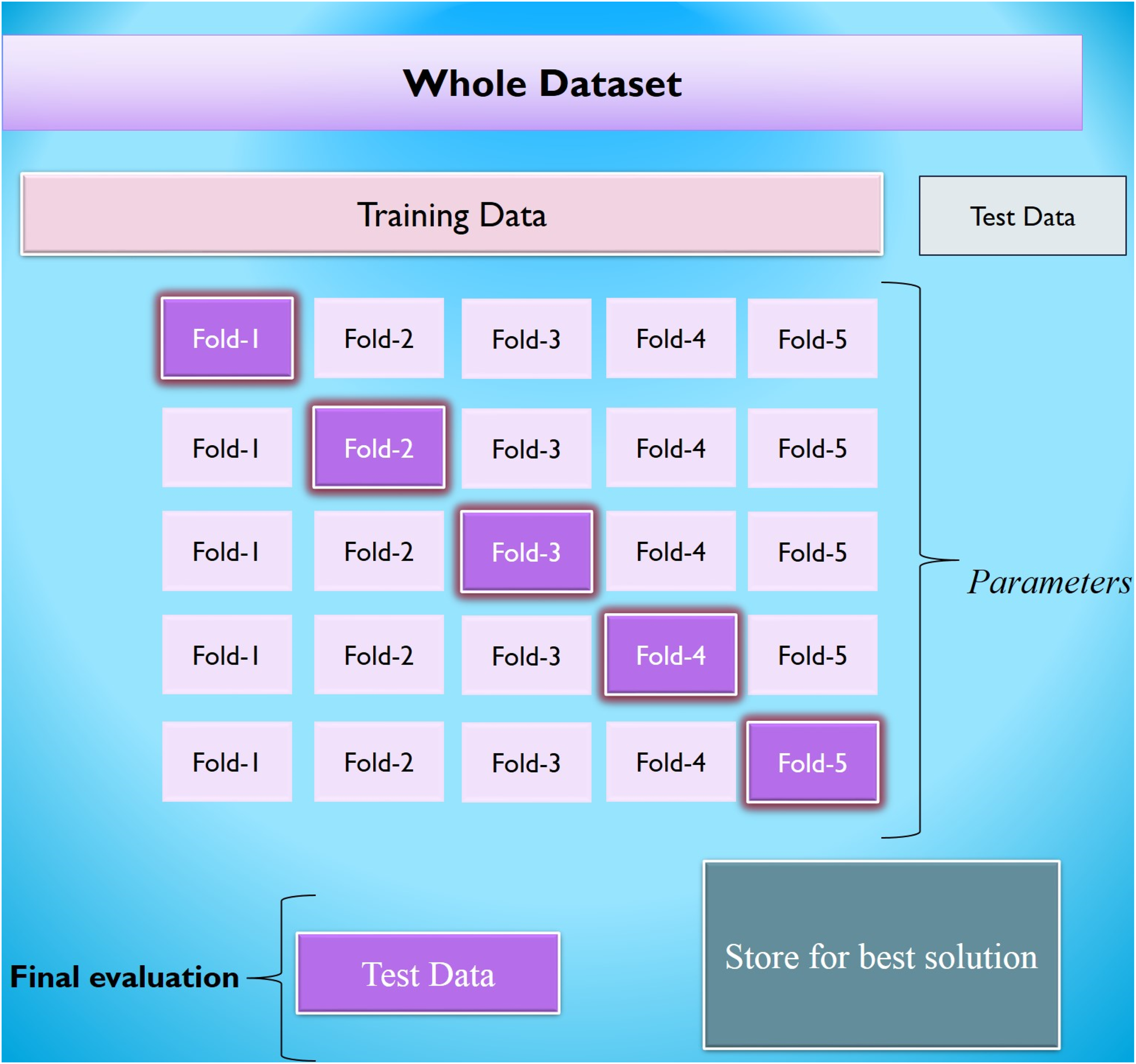
Schematic diagram for K-fold approach.

By systematically rotating which fold is used for testing, K-fold cross-validation provides a more comprehensive and robust measure of model performance. This approach helps minimize issues related to overfitting or bias that can arise from relying on a single train-test split, thereby supporting more confident selection and tuning of machine learning models (Buran and Erçek, 2022; Vujović, 2021).

To evaluate the predictive accuracy and overall performance of each model, several critical metrics were computed: relative error percentage (RE%), average absolute relative error percentage (AARE%), mean squared error (MSE), and the coefficient of determination (R²). The subsequent sections provide detailed descriptions of each of these evaluation criteria (Abbasi et al., 2023; Hasanzadeh and Madani, 2024; Madani and Alipour, 2022; Madani et al., 2021):

R E % = (\frac{V^{p r e d} - V^{\exp}}{V^{\exp}}) \times 100

(8 )

A A R E % = \frac{100}{N} \sum_{i = 1}^{N} (| \frac{V_{i}^{p r e d} - V_{i}^{\exp}}{V_{i}^{\exp}} |)

(9 )

M S E = \frac{\sum_{i = 1}^{N} {(V_{i}^{p r e d} - V_{i}^{\exp})}^{2}}{N}

(10 )

R^{2} = 1 - \frac{\sum_{i = 1}^{N} {(V_{i}^{p r e d} - V_{i}^{\exp})}^{2}}{\sum_{i = 1}^{N} {(V_{i}^{\exp} - \bar{V})}^{2}}

(11 )

Within the following equations, the subscript iii identifies a specific data point in the dataset. The symbols “pred” and “exp” correspond to the predicted value and the actual (experimental) value for that data point, respectively. The variable N indicates the total number of data points considered.

Models’ evaluation

To evaluate errors and judge how well the model performed, three statistical indicators were applied: MSE, R², and AARE%. These metrics are widely recognized for their ability to systematically measure how accurate, reliable, and predictive computational models. MSE calculates the average of the squared differences between the model's predictions and actual observed values, emphasizing larger errors more heavily and offering insight into the typical magnitude of prediction mistakes. R², on the other hand, demonstrates how well the model explains variations in the observed data, quantifying the proportion of total outcome variability that can be attributed to the input variables. The AARE% expresses, as a percentage, the mean relative error, making it easier to interpret the model's average error in relation to actual data.

Using this combination of statistical tools allows for a thorough model assessment—considering not just total error, but also how much of the variance in the outcome is captured by the model. As such, these metrics are considered essential for a robust and meaningful evaluation of predictive model performance (Madani et al. 2017 , 2021):

Results and discussion

Correlation analysis

Figure 4 illustrates the Pearson correlation matrix, which was derived by computing Pearson's correlation coefficients for every pair of variables analyzed in this research. Pearson's correlation coefficient (r) quantifies the degree and direction of linear association between two continuous variables, taking values from −1 to +1. An r value of +1 signifies a perfect direct relationship, −1 corresponds to a perfect inverse relationship, and 0 indicates an absence of linear correlation.

Figure 4.

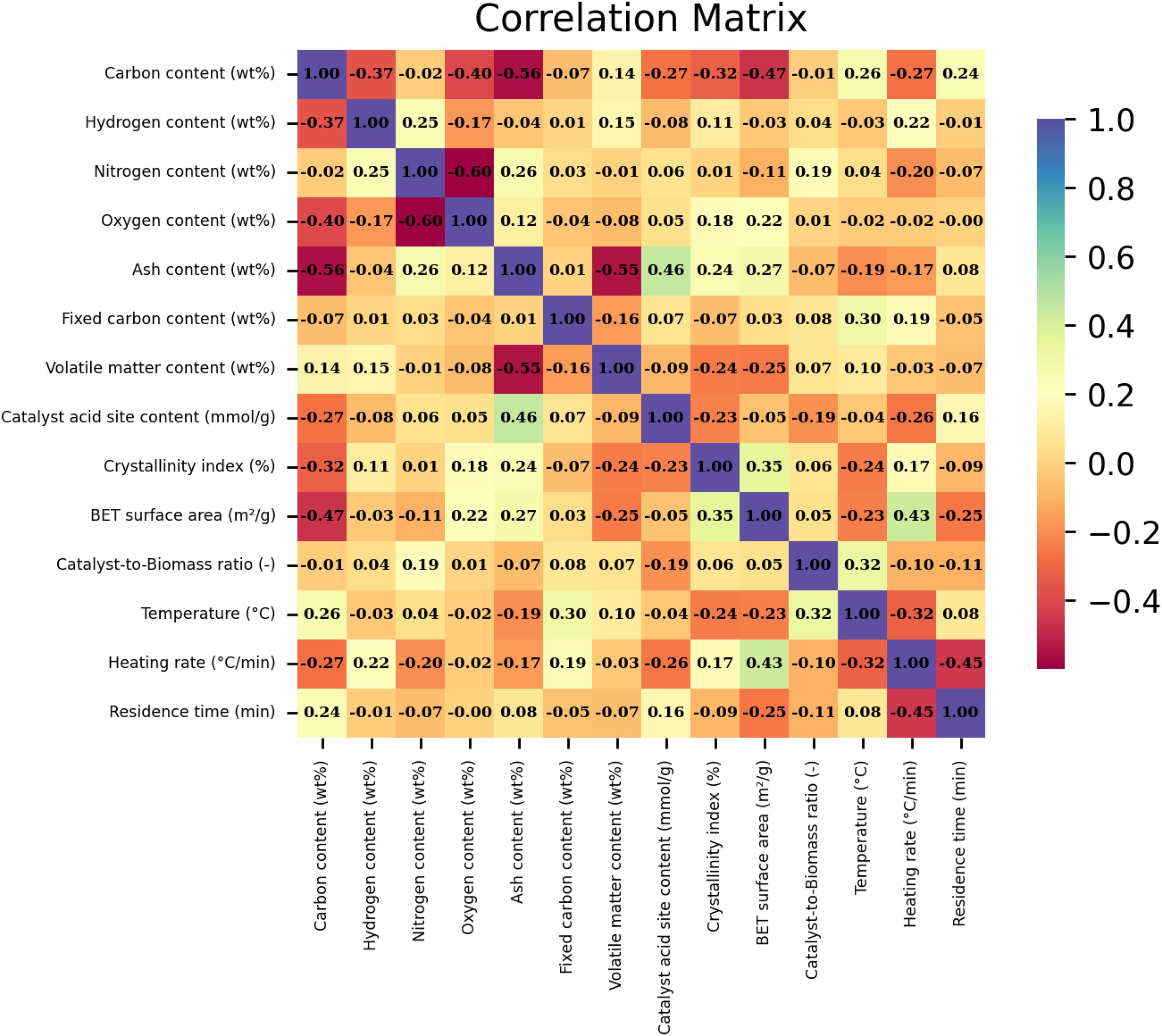
Pearson correlation matrix illustrating the linear relationships among input variables and biochar yield in biomass pyrolysis.

This matrix serves as a comprehensive tool to visualize and interpret the linear interdependencies among all studied parameters, including both input features and the output variable, biochar yield, resulting from the pyrolysis of biomass. Through this analysis, researchers gain a clearer understanding of which variables are most influential in predicting biochar production outcomes.

Reviewing the correlation matrix in Figure 4, it is evident that certain input factors, such as ash content, catalyst acid site concentration, and residence time, exhibit pronounced positive correlations with biochar yield. This suggests that increases in these variables are generally associated with greater biochar production under the examined conditions. Conversely, variables like heating rate and pyrolysis temperature display strong negative correlations with yield, implying that higher levels of these parameters tend to reduce biochar formation.

It is also worth noting that, relative to these five variables, the remaining factors considered in the study have much weaker correlations with yield, indicating a more negligible direct effect on biochar output within the modeled parameter space. Ultimately, constructing and analyzing the Pearson correlation matrix enables the identification of key determinants of yield variability, supporting more targeted optimization in biomass pyrolysis processes.

Data quality validation

The leverage method is a robust diagnostic tool used to pinpoint unusual or potentially influential data points in regression analysis. It operates by integrating the standard deviation of residuals with the so-called Hat matrix (H), which reflects how data points impact the overall regression fit. The Hat matrix is mathematically defined as follows (Madani et al., 2021) :

H = X (X^{T} X)^{- 1} X^{T}

(12)

Here, X denotes the design matrix, with X^T representing its transpose. The diagonal elements of the Hat matrix quantify the influence each observation exerts on the regression estimates. As such, observations with unusually high leverage can disproportionately affect the calibration of the model.

To discern which leverage values are considered significant, a threshold (H*) is commonly established based on the number of input variables (n) and the number of total samples (m m m), using the expression (Bemani et al., 2023):

H * = 3 (n + 1) / m

(13)

Data points with leverage values exceeding this threshold are flagged for further scrutiny, as they may indicate outliers or influential cases that could compromise the quality of the regression model. This assessment is often visualized using a Williams plot, as illustrated in Figure 5. The plot highlights reliable regions enclosing most of the data, while points breaching the suspicion thresholds (often less than 1% of the data, shown in yellow) are labeled as potentially problematic.

Figure 5.

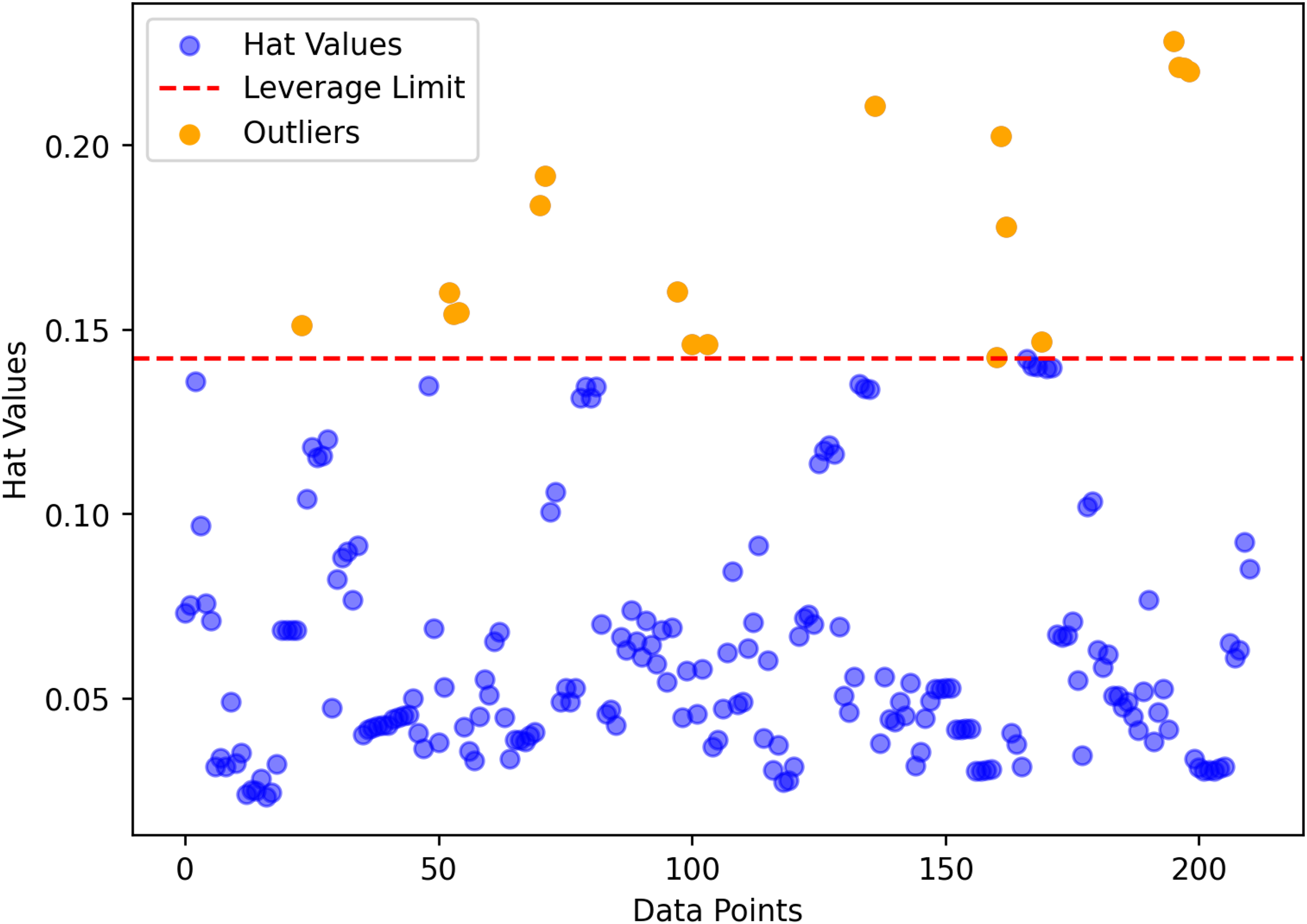
Williams plot displaying leverage values and outlier boundaries for identifying influential data points in the regression model.

By systematically analyzing leverage values, researchers can ensure the integrity and stability of their predictive models. Identifying influential outliers allows for more accurate generalization and reduces the risk of skewed or unreliable predictions, ultimately enhancing the model's overall performance and reliability.

Models’ optimization

Table 1 presents the comprehensive tuning of key GBDT hyperparameters—such as number of estimators, tree depth, feature fraction, and learning rate by four different optimization techniques: GPO, ES, BPI, and BBO. Each optimization algorithm was employed to systematically search a defined range for each parameter, both independently and with cross-validation, in order to maximize model performance. The optimal values selected by each technique demonstrate clear differences, reflecting the unique search strategies and heuristic principles underlying each algorithm.

Table 1.

Considered parameter ranges and optimized GBDT hyperparameters selected by four different optimization algorithms.

Tuning parameter	Considered range	GPO	ES	BPI	BBO
n_estimators	[50–300]	283	173	180	222
max_depth	[5–20]	16	13	14	12
max_features	[0.1–1]	0.957	0.558	0.805	0.690
min_samples_split	[0.01–0.5]	0.043	0.093	0.052	0.155
learning_rate	[0.01–0.3]	0.271	0.175	0.208	0.243
subsample	[0.5–1]	0.604	0.740	0.789	0.772
min_samples_leaf	[0.01–0.5]	0.022	0.019	0.013	0.017

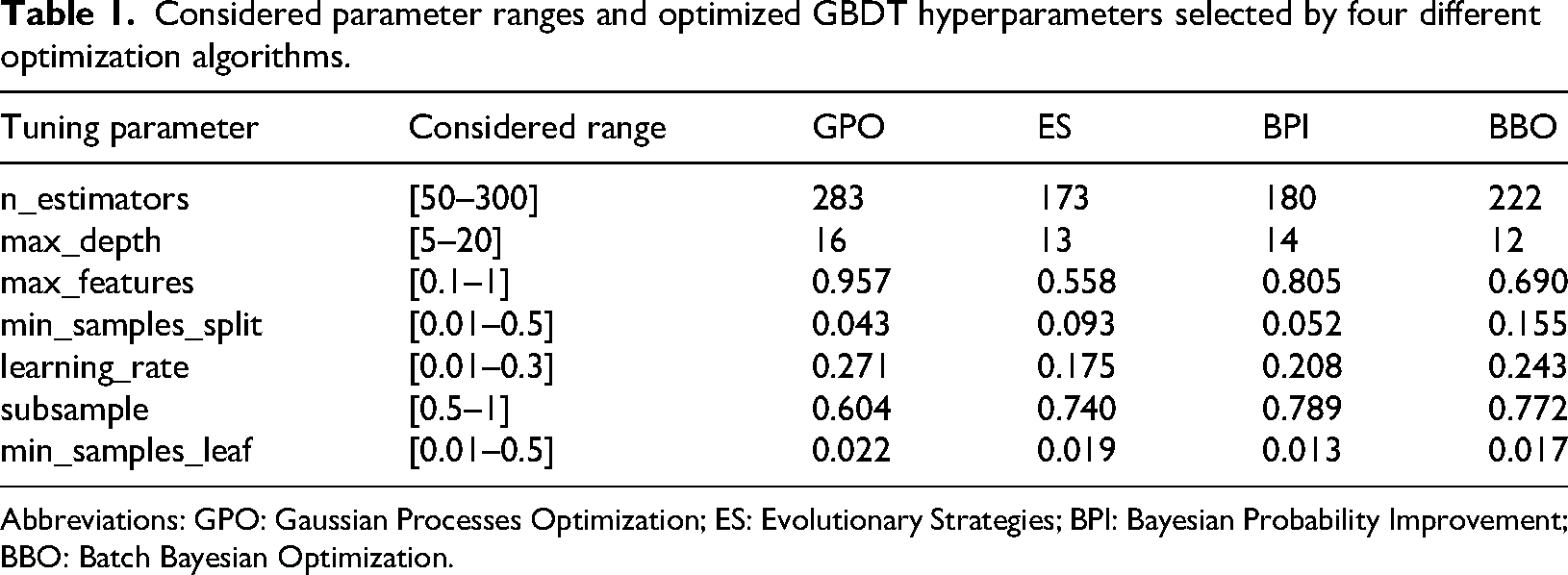
Abbreviations: GPO: Gaussian Processes Optimization; ES: Evolutionary Strategies; BPI: Bayesian Probability Improvement; BBO: Batch Bayesian Optimization.

These results highlight the impact that the choice of optimization method can have on the configuration and complexity of machine learning models. While GPO tended to favor higher model complexity, ES and BBO found comparatively more regularized solutions. Such variations influence both predictive ability and generalization. The comparative analysis underscores the value of applying advanced optimization strategies for hyperparameter tuning in the GBDT framework, as this leads to more robust and reliable performance in predicting biochar yield from biomass pyrolysis data.

Figure 6 provides a comparative visualization of the optimization trajectories for each algorithm by plotting the MSE values across 500 trial iterations. This figure enables the direct assessment of each optimizer's efficiency and convergence trends as they search for the most effective GBDT hyperparameters. The highlighted points in the plots indicate the hyperparameter settings at which the optimizers achieve their lowest MSE, serving as visual evidence of the solution quality and search behaviors.

Figure 6.

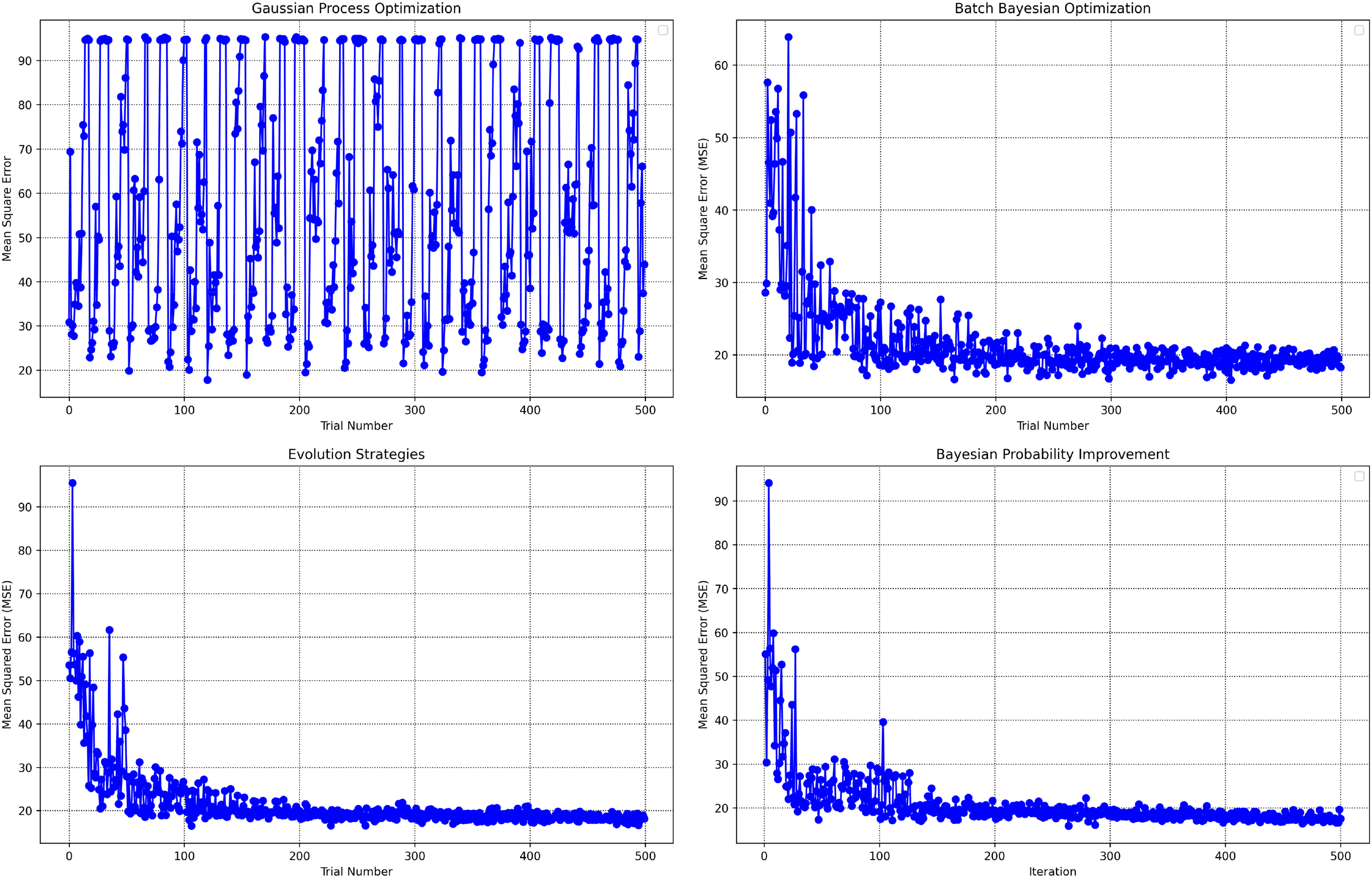
Optimization trajectories of mean squared error across 500 iterations for each algorithm.

A notable distinction emerges in the performance patterns among the algorithms. The GPO algorithm exhibits highly fluctuating MSE values throughout the optimization process, indicating less consistent progress toward error minimization and an absence of smooth convergence. In contrast, ESs, BPI and BBO all demonstrate rapid convergence, with the MSE sharply decreasing and stabilizing to its lowest value, usually within the first 100 iterations. This suggests that, for this application, these three methods are notably more effective and efficient at finding optimal hyperparameters compared to GPO, reflecting their adaptability and robustness in model tuning tasks.

Figure 7 presents a comparative analysis of the computational times for each optimization algorithm, measured over 500 iterations on a standardized hardware setup equipped with 16 GB RAM and an Intel Core i7-6700 processor (3.40 GHz). The results reveal that, while all four algorithms demonstrate comparable optimization times, the BBO method stands out as the most time-consuming, taking roughly 313 s to complete the process. Conversely, the GPO consistently registers as the fastest, achieving the shortest overall runtime. Despite these differences, the actual variation in computational time among the methods is relatively minor, indicating that all four optimizers offer similar levels of computational efficiency when applied to this specific machine learning task.

Figure 7.

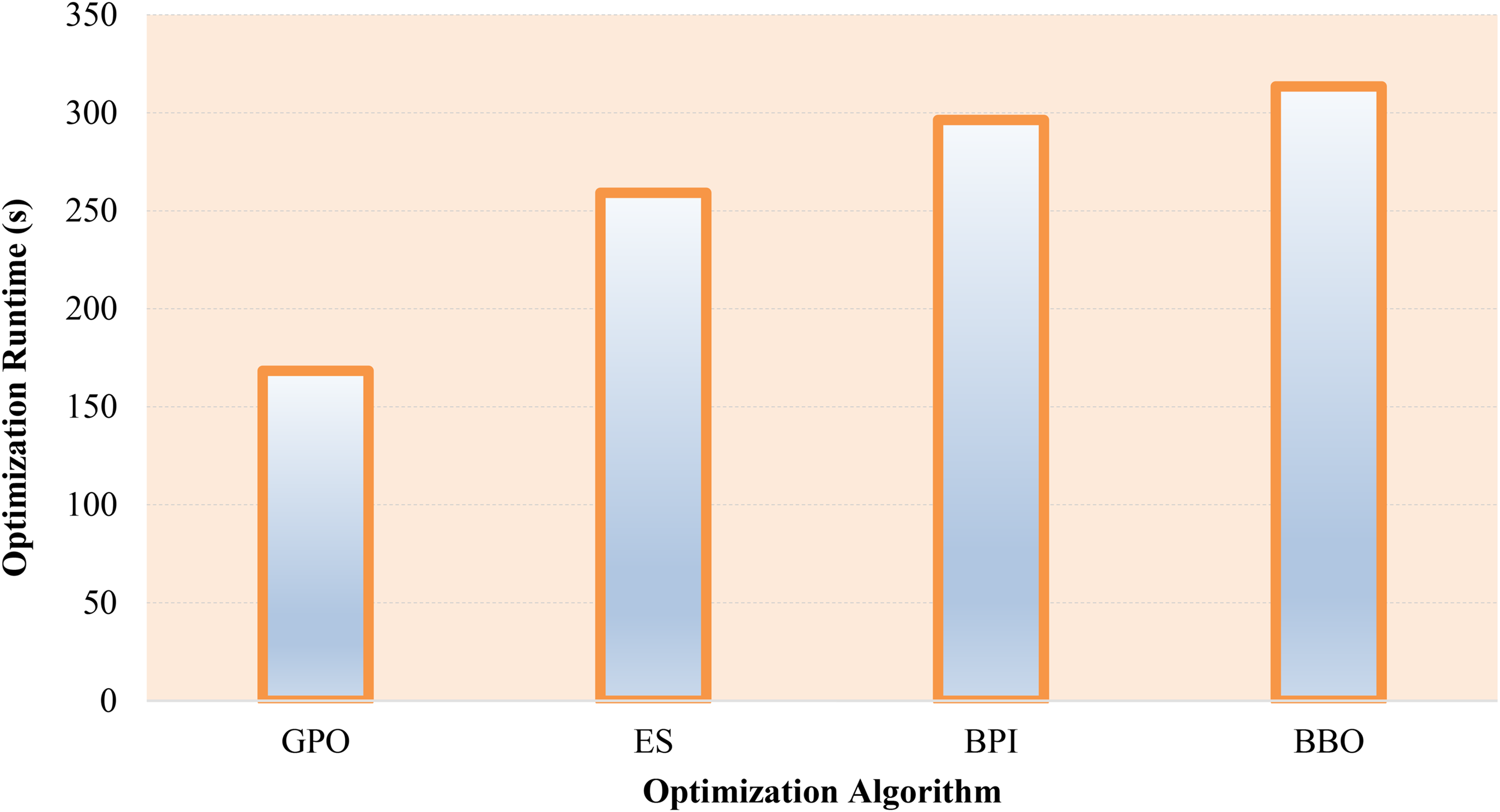
Computational time for each optimization method over 500 iterations on identical hardware.

Table 2 presents a quantitative evaluation of GBDT models tuned by four optimization algorithms, highlighting clear performance differences. GBDT–BPI achieves the highest total R² value at 0.9816, surpassing GBDT–GPO (0.9776), GBDT–BBO (0.9797), and GBDT–ES (0.9762). For MSE, GBDT–BPI records the lowest total value of 1.65, compared to 2.01 for GBDT–GPO, 1.81 for GBDT–BBO, and 2.13 for GBDT–ES. Similarly, AARE% for GBDT–BPI is the lowest at 1.35%, followed by GBDT–GPO (1.72%), GBDT–BBO (2.58%), and GBDT–ES (3.81%).

Table 2.

Performance metrics of GBDT models optimized by different algorithms, evaluated by R², MSE, and AARE% on training, test, and total datasets.

Optimization algorithm	R2			MSE			AARE%
Optimization algorithm	Training	Test	Total	Training	Test	Total	Training	Test	Total
GBDT–GPO	0.998755	0.6320008	0.977597	0.116883	18.250978	2.007641	0.774037	9.8288786	1.718144
GBDT–ES	0.996829	0.6394417	0.976217	0.297838	17.881945	2.131252	3.064016	10.201492	3.808208
GBDT–BPI	0.999268	0.6933671	0.981619	0.068709	15.207505	1.647162	0.392632	9.5377828	1.346155
GBDT–BBO	0.998072	0.6803927	0.979748	0.181039	15.850971	1.814871	1.872033	8.6631931	2.580116

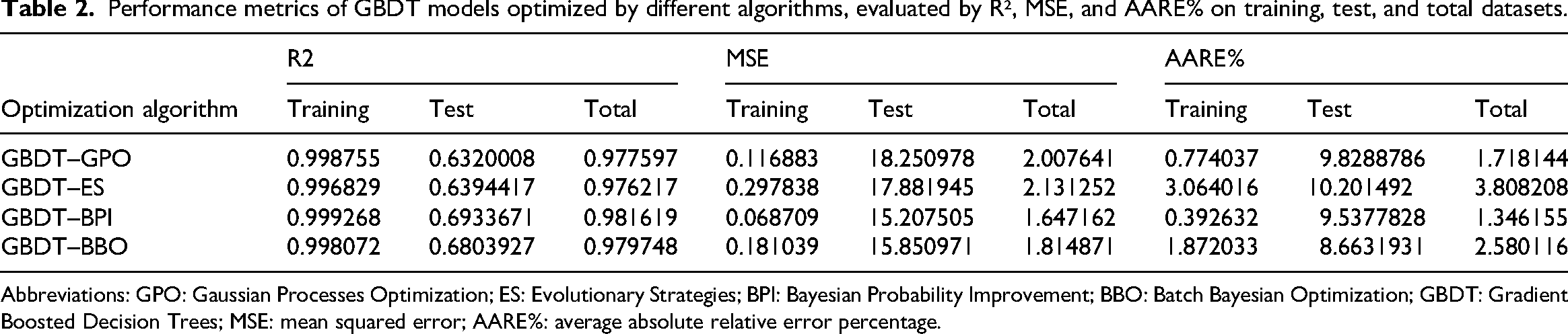
Abbreviations: GPO: Gaussian Processes Optimization; ES: Evolutionary Strategies; BPI: Bayesian Probability Improvement; BBO: Batch Bayesian Optimization; GBDT: Gradient Boosted Decision Trees; MSE: mean squared error; AARE%: average absolute relative error percentage.

These results show that the GBDT–BPI model not only fits the training data well but also maintains its predictive accuracy on the test data, with test R² of 0.6934 and test MSE of 15.21, both better than the other algorithms. This quantitative evidence indicates that GBDT–BPI provides the most accurate and robust prediction performance among the compared methods, making it the preferred choice for model tuning and deployment based on this study.

Figure 8 illustrates the crossplots of actual versus predicted target values generated by various machine learning models, providing a visual assessment of model accuracy and fit. This figure emphasizes the degree to which each model's predictions align with the ideal y = x line, which represents perfect correspondence between observed and predicted values. Among the models compared, the GBDT combined with the BPI optimizer displays predictions that are tightly clustered around both the best-fit regression line and the y = x reference, indicating minimal dispersion and excellent predictive alignment.

Figure 8.

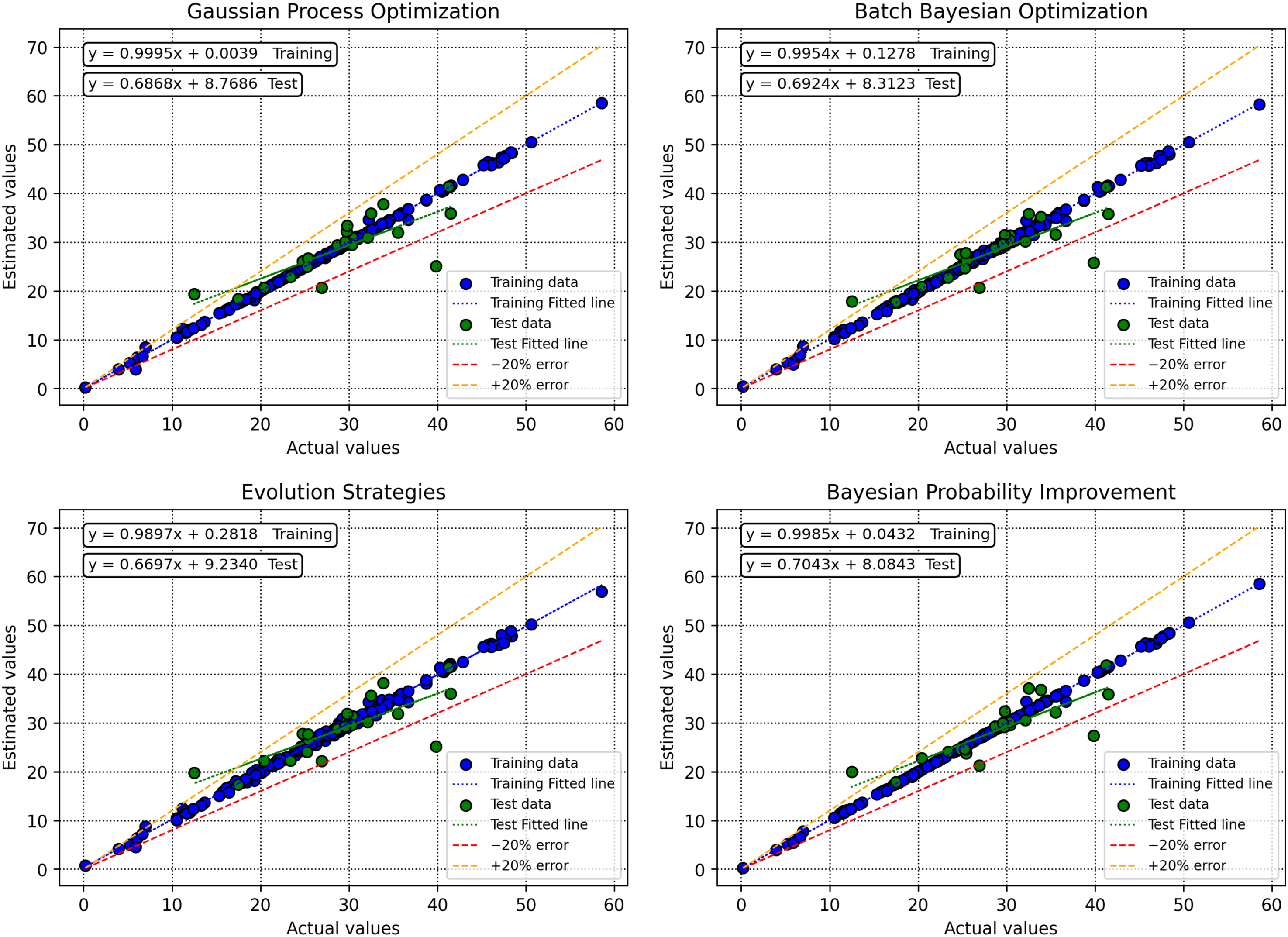
Crossplots of observed versus predicted target values for different machine learning models.

Figure 9 presents the RE% for each data point across the different machine learning approaches. The plot highlights the consistency and stability of the predictive models, with a particular focus on error distribution relative to the zero-error baseline (y = 0 line). Notably, when GBDT is coupled with BPI, the data points exhibit relative errors that are densely concentrated near zero, reflecting not only improved reliability but also enhanced generalization in model predictions compared to the other approaches.

Figure 9.

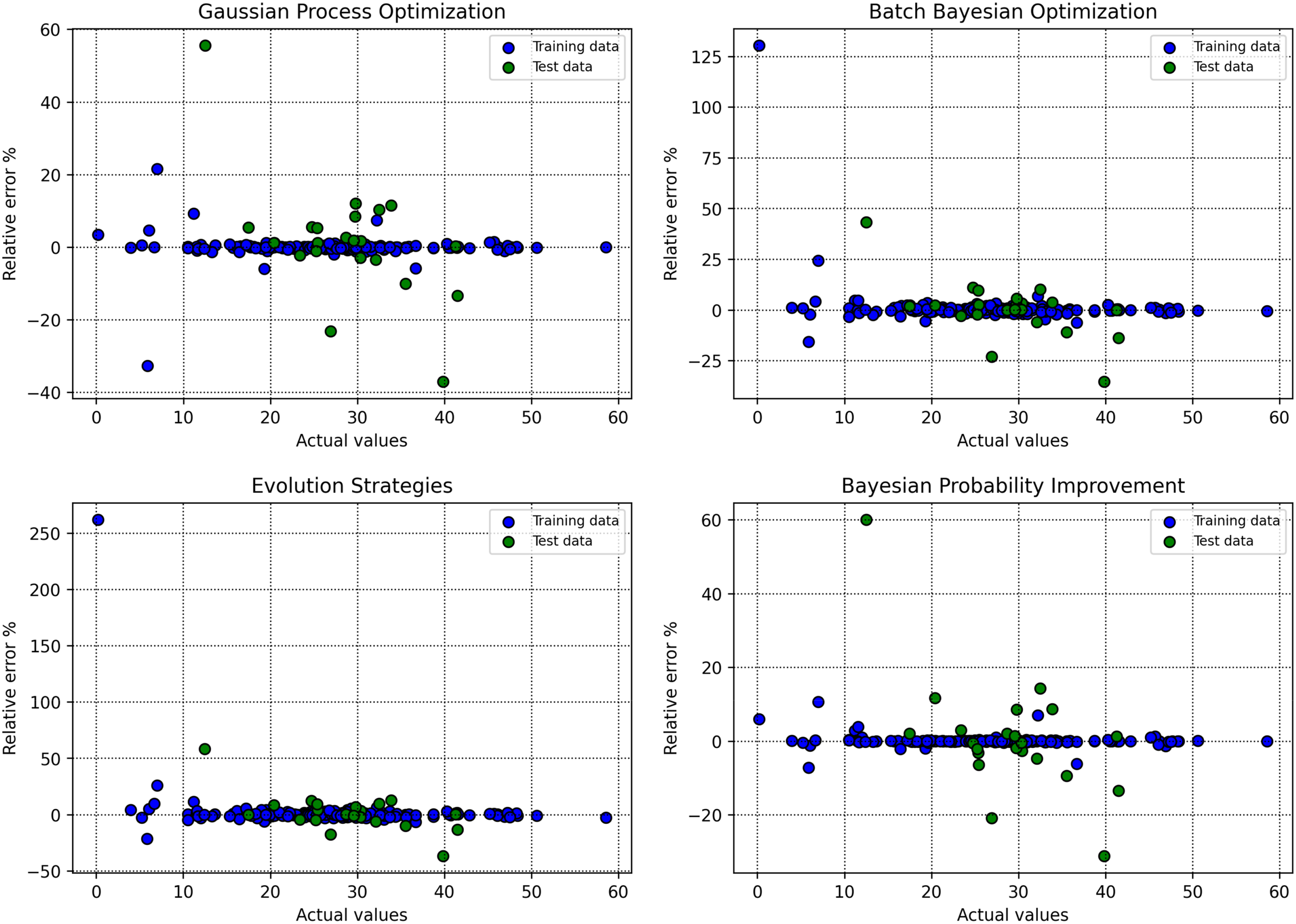
Relative error percentages for each data point across various machine learning models.

Figure 10 visually compares the predicted versus actual target values for each data point, as generated by the machine learning models tuned with different optimization techniques. Each model's performance is displayed within a single diagram, providing a direct comparison of how closely the predicted outputs align with the ground truth across the sample set. Notably, the GBDT–BPI combination demonstrates visibly reduced dispersion between predicted and real values, with data points clustering tightly around the respective reference line, suggesting a more precise model fit. This comprehensive plot offers a clear overview of each optimization algorithm's capacity to generalize and accurately predict unseen data, facilitating an objective visual evaluation of prediction accuracy in a single consolidated view.

Figure 10.

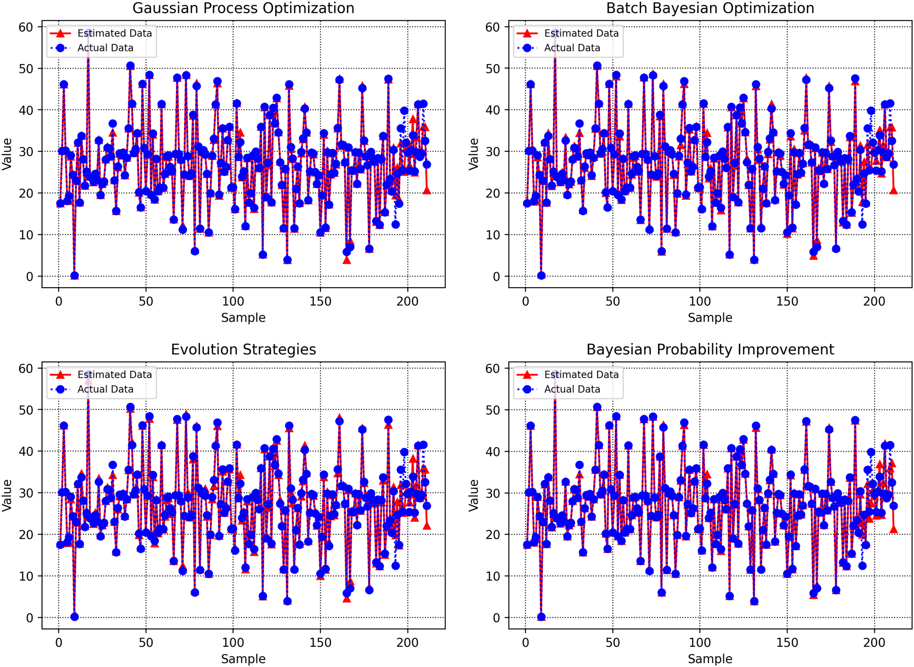
Comparison of predicted and observed target values for each optimization algorithm in a unified diagram.

The SHAP feature importance diagram, presented in Figure 11, offers a comprehensive ranking of the influence exerted by each input parameter on the output variable within the model. By sorting features in descending order of their SHAP scores, the diagram provides clear insight into the relative contribution of every variable, supporting interpretability and transparency in the machine learning process. This method quantifies the average impact of each feature on model predictions, allowing researchers to discern which input variables are most critical in driving the output.

Figure 11.

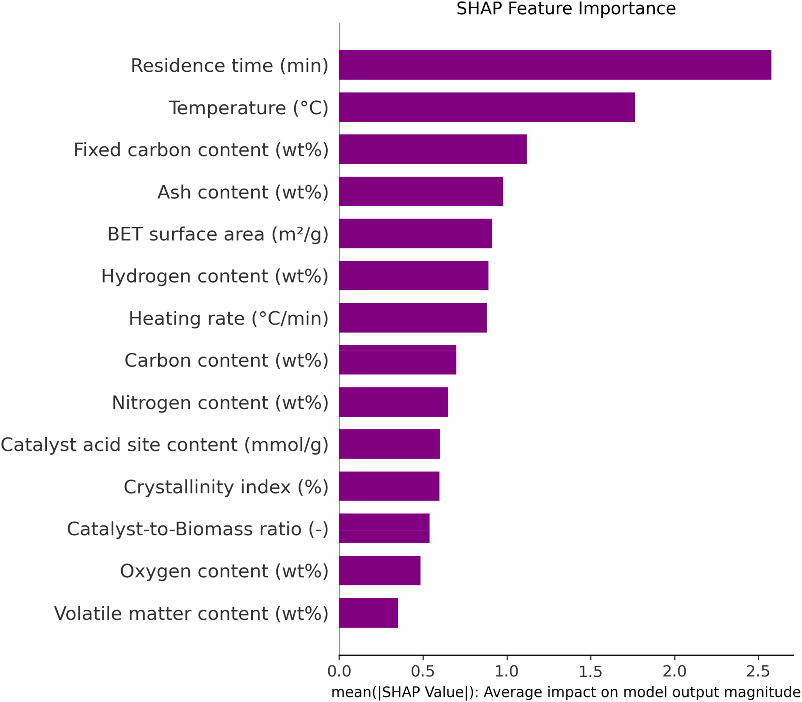
SHAP feature importance ranking of input variables for predicting biochar yield in biomass pyrolysis.

According to the diagram, reside duration, temperature, and fixed carbon content emerge as the top contributors affecting biochar yield from the pyrolysis of biomass. The SHAP analysis systematically highlights these parameters as having the highest importance values compared to other features, such as ash content, catalyst acid site concentration, or heating rate, which appear lower in the ranking. Such a feature importance breakdown is valuable for both model refinement and practical process optimization, guiding researchers to focus on the most influential operational conditions when aiming to improve biochar yield in future studies.

Figure 12 provides a SHAP feature contribution plot, where each point represents the impact of a feature value on the model's predicted output. Red points correspond to high values of a feature, while blue points indicate low values. By visualizing the spread and direction of these contributions, the plot enables a detailed breakdown of how individual high or low feature values drive the model's predictions either positively or negatively. This type of visualization is particularly useful for interpreting complex machine learning models, as it makes clear not only which features are influential, but also how their value ranges affect the outcome.

Figure 12.

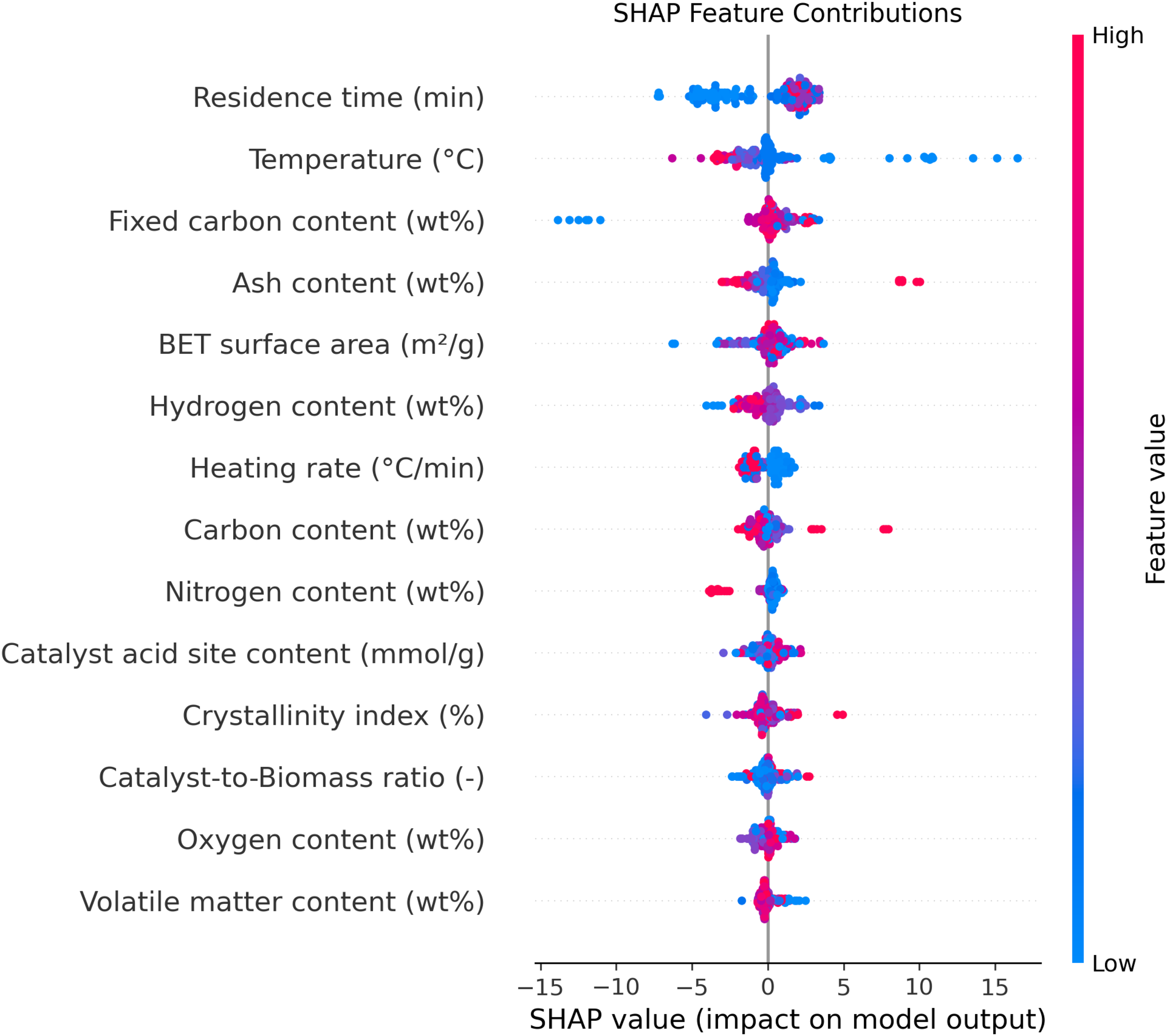
SHAP summary plot visualizing individual feature contribution to biochar yield, colored by feature value for each parameter.

Focusing on the observed trends, the SHAP plot shows that higher values (red points) for residence time cluster on the positive side of the contribution scale, indicating that increased residence time leads to higher biochar yield. This aligns with the theory that prolonged exposure during pyrolysis allows for more complete conversion of biomass to biochar. In contrast, the red points for temperature are predominantly on the negative side, demonstrating that higher temperatures correspond with decreased biochar yield. Theoretically, this can be attributed to the fact that, at elevated temperatures, volatile compounds are more readily released and less solid biochar is formed, shifting the product distribution toward bio-oil and syngas rather than solid yield. Together, the plot and these theoretical considerations provide a nuanced understanding of how process variables govern biochar production efficiency.

Novelty and contribution

Recent studies have shown the promise of machine learning for predicting biochar yield from biomass pyrolysis, employing methods such as Random Forests, neural networks, and ensemble learning, often combined with feature sensitivity analysis and optimization techniques. For example Zhu et al. (2019) and Ma et al. (2023) demonstrated the value of ML in capturing feature–output relationships and highlighted temperature as a decisive variable, while Li et al. (2022a) and Ul Haq et al. (2022) evaluated diverse ML architectures with classical optimization algorithms (e.g. GA, PSO), reporting strong prediction metrics (e.g. ELT-PSO with R² = 0.99). Further Kanthasamy et al. (2023) and Sait et al. (2025) explored hybrid and ANN models, focusing on process variables like residence time and nitrogen flow, but often restricted their analysis to a single optimization protocol, limited hyperparameter rigor, or fewer feature evaluation methods.

The distinctive contribution of the present study lies in three aspects: (i) the integration and comparative benchmarking of multiple advanced hyperparameter optimization algorithms (GPO, ES, BPI, BBO) specifically for GBDT—an approach not systematically covered in earlier biochar modeling works; (ii) the use of an extensive, literature-derived dataset (211 samples, 14 features) that supports broader generalization and model stability analysis; and (iii) a comprehensive, multilayered interpretability pipeline including both correlation-based sensitivity and SHAP value-based feature attribution. This multifaceted workflow not only yields state-of-the-art accuracy (GBDT–BPI: total R² = 0.982, MSE = 1.65, AARE% = 1.35), but also uniquely quantifies optimizer efficiency and the effect of parameter tuning strategies on model reliability. By offering an open methodology that combines rigorous validation, multiple optimization pathways, and transparent feature importance mapping, this research directly advances the field's capacity to produce reliable, actionable predictions for biochar output and facilitates practical process improvements.

Despite substantial improvements in predictive accuracy using advanced optimization techniques, some limitations remain. The diversity and representativeness of the dataset, as well as the inherent complexity of biochar production, may affect model generalizability to new biomass types or process conditions. Future studies should consider expanding the dataset and exploring additional model architectures or multisource data integration to further improve robustness and universal applicability.

Conclusions

This study successfully developed and validated a predictive framework for biochar yield in biomass pyrolysis using an extensive literature-based dataset and advanced machine learning techniques. By leveraging GBDT models and systematically optimizing their hyperparameters through four different algorithms, Bayesian Probability Improvement emerged as the most effective approach, achieving both the highest R² and the lowest prediction errors across training and testing sets. The workflow integrated sensitivity analysis, leverage diagnostics, and SHAP-based feature importance, collectively highlighting residence time, pyrolysis temperature, and fixed carbon content as pivotal determinants of yield. The robustness of the framework, confirmed by multiple validation approaches, underscores its utility for both researchers and industry practitioners aiming to enhance process efficiency. However, limitations include the reliance on literature-sourced data with inherent heterogeneity and potential unmeasured confounders, as well as model generalizability restricted to the range represented in the dataset. Future research should prioritize expanding the dataset with experimental and field-scale data, exploring additional modeling paradigms (e.g. deep learning), and implementing real-time process optimization to further improve predictive accuracy and operational relevance.

Supplemental Material

sj-xlsx-1-eea-10.1177_01445987251359321 - Supplemental material for Accurate modeling of biochar yield based on proximate analysis

Supplemental material, sj-xlsx-1-eea-10.1177_01445987251359321 for Accurate modeling of biochar yield based on proximate analysis by Walid Abdelfattah, Munthar Kadhim Abosaoda, Krunal Vaghela, Gowrishankar J, Prabhat Kumar Sahu, Kamred Udham Singh, R Sivaranjani and Samim Sherzod in Energy Exploration & Exploitation

Footnotes

ORCID iD

Samim Sherzod

Funding

The authors disclosed receipt of the following financial support for the research, authorship, and/or publication of this article: The authors extend their appreciation to the Deanship of Scientific Research at Northern Border University, Arar, KSA, for funding this research work through the project number NBU-FFR-2025-2230-20.

Declaration of conflicting interests

The authors declared no potential conflicts of interest with respect to the research, authorship, and/or publication of this article.

Data availability statement

Data is available in the supplementary material excel file.

Supplemental material

Supplemental material for this article is available online.

References

Abbasi

Aghdam

SK-Y

Madani

(2023) Modeling subcritical multi-phase flow through surface chokes with new production parameters. Flow Measurement and Instrumentation 89: 102293.

Allohverdi

Mohanty

Roy

, et al. (2021) A review on current status of biochar uses in agriculture. Molecules 26(18): 5584.

Ament

Daulton

Eriksson

, et al. (2023) Unexpected improvements to expected improvement for Bayesian optimization. Advances in Neural Information Processing Systems 36: 20577–20612.

Azimi

Jalali

Fern

(2012) Hybrid batch Bayesian optimization. arXiv preprint arXiv:1202.5597.

Bemani

Madani

Kazemi

(2023) Machine learning-based estimation of nano-lubricants viscosity in different operating conditions. Fuel 352: 129102.

Beyer

H-G

Schwefel

H-P

(2002) Evolution strategies–A comprehensive introduction. Natural Computing 1: 3–52.

Börjesson

PII

(1996) Energy analysis of biomass production and transportation. Biomass and Bioenergy 11(4): 305–318.

Brown

Wright

Brown

(2011) Estimating profitability of two biochar production scenarios: Slow pyrolysis vs fast pyrolysis. Biofuels, Bioproducts and Biorefining 5(1): 54–68.

Buran

Erçek

(2022) Public transportation business model evaluation with spherical and intuitionistic fuzzy AHP and sensitivity analysis. Expert Systems with Applications 204: 117519.

10.

Canam

Town

Iroba

, et al. (2013) Pretreatment of Lignocellulosic Biomass Using Microorganisms: Approaches, Advantages, and Limitations. London, UK: IntechOpen.

11.

Chaihad

Anniwaer

Karnjanakom

, et al. (2021) In-situ catalytic upgrading of bio-oil derived from fast pyrolysis of sunflower stalk to aromatic hydrocarbons over bifunctional Cu-loaded HZSM-5. Journal of Analytical and Applied Pyrolysis 155: 105079.

12.

Elkhalifa

Al-Ansari

Mackey

, et al. (2019) Food waste to biochars through pyrolysis: A review. Resources, Conservation and Recycling 144: 310–320.

13.

Farid

Rahman

(2010) Anomaly network intrusion detection based on improved self adaptive Bayesian algorithm. Journal of Computers 5(1): 23–31.

14.

Fransen

De Kroon

(2001) Long-term disadvantages of selective root placement: Root proliferation and shoot biomass of two perennial grass species in a 2-year experiment. Journal of Ecology 89(5): 711–722.

15.

Garcia

Caraschi

Ventorim

, et al. (2019) Assessment of plant biomass for pellet production using multivariate statistics (PCA and HCA). Renewable Energy 139: 796–805.

16.

González

Dai

Hennig

, et al. Batch Bayesian optimization via local penalization, PMLR.

17.

Gurevich Messina

Bonelli

Cukierman

(2017) In-situ catalytic pyrolysis of peanut shells using modified natural zeolite. Fuel Processing Technology 159: 160–167.

18.

Hansen

Arnold

Auger

(2015) Evolution strategies. In: Springer Handbook of Computational Intelligence. Berlin, Heidelberg: Springer , 871–898.

19.

Haq

Ullah

Khan

MNA

, et al. (2022) Comparative study of machine learning methods integrated with genetic algorithm and particle swarm optimization for bio-char yield prediction. Bioresource Technology 363: 128008.

20.

Hasanzadeh

Madani

(2024) Deterministic tools to predict gas assisted gravity drainage recovery factor. Energy Geoscience 5(3): 100267.

21.

Hatefirad

Hosseini

Tavasoli

(2022) Effect of Fe/Cu catalysts supported on zeolite/active carbon hybrid on bio-oil quality derived from catalytic pyrolysis of granular bacteria biomass. Fuel 312: 122870.

22.

Heinimö

Junginger

(2009) Production and trading of biomass for energy–an overview of the global status. Biomass and Bioenergy 33(9): 1310–1320.

23.

Jahan

Ullah

SMI

Aminun

, et al. (2024) Effect of sterile rice spikelets derived biochar amendment on nutrient leaching and availability in paddy soil under continuous standing water. Geology, Ecology, and Landscapes 8(4): 574–582.

24.

Jenkins

(2015) Estimating ecological production from biomass. Ecosphere (Washington, D C) 6(4): 1–31.

25.

Jha

Biswas

Lakaria

, et al. (2010) Biochar in agriculture–prospects and related implications. Current Science 99: 1218–1225.

26.

Jiang

Cai

Wang

, et al. (2012) Improving tree augmented naive Bayes for class probability estimation. Knowledge-Based Systems 26: 239–245.

27.

Kanthasamy

Almatrafi

Ali

, et al. (2023) Biochar production from valorization of agricultural wastes: Data-driven modelling using machine learning algorithms. Fuel 351: 128948.

28.

Khezerloo-ye Aghdam

Kazemi

Ahmadi

(2023) Theoretical and experimental study of fine migration during low-salinity water flooding: Effect of brine composition on interparticle forces. SPE Reservoir Evaluation & Engineering 26(02): 228–243.

29.

Khezerloo-ye Aghdam

Kazemi

Ahmadi

(2024) Studying the effect of surfactant assisted low-salinity water flooding on clay-rich sandstones. Petroleum 10(2): 306–318.

30.

Khezerlooe-ye Aghdam

Moslemizadeh

Madani

, et al. (2019) Mechanistic assessment of Seidlitzia rosmarinus-derived surfactant for restraining shale hydration: A comprehensive experimental investigation. Chemical Engineering Research and Design 147: 570–578.

31.

Laird

Brown

Amonette

, et al. (2009) Review of the pyrolysis platform for coproducing bio-oil and biochar. Biofuels, Bioproducts and Biorefining 3(5): 547–562.

32.

Laitila

Virtanen

(2016) Improving construction of conditional probability tables for ranked nodes in Bayesian networks. IEEE Transactions on Knowledge and Data Engineering 28(7): 1691–1705.

33.

Gupta

You

(2022a) Machine learning assisted prediction of biochar yield and composition via pyrolysis of biomass. Bioresource Technology 359: 127511.

34.

Gupta

Zhang

, et al. (2023) Review of biochar production via crop residue pyrolysis: Development and perspectives. Bioresource Technology 369: 128423.

35.

Nishu Yellezuome

, et al. (2022b) Deactivation mechanism and regeneration effect of bi-metallic Fe-Ni/ZSM-5 catalyst during biomass catalytic pyrolysis. Fuel 312: 122924.

36.

Liu

, et al. (2021) Improved naive Bayesian probability classifier in predictions of nuclear mass. Physical Review C 104(1): 014315.

37.

Zhang

Liu

, et al. (2023) Machine learning prediction of biochar yield based on biomass characteristics. Bioresource Technology 389: 129820.

38.

Madani

Abbasi

Baghban

, et al. (2017) Modeling of CO2-brine interfacial tension: Application to enhanced oil recovery. Petroleum Science and Technology 35(23): 2179–2186.

39.

Madani

Alipour

(2022) Gas-oil gravity drainage mechanism in fractured oil reservoirs: Surrogate model development and sensitivity analysis. Computational Geosciences 26(5): 1323–1343.

40.

Madani

Moraveji

Sharifi

(2021) Modeling apparent viscosity of waxy crude oils doped with polymeric wax inhibitors. Journal of Petroleum Science and Engineering 196: 108076.

41.

Mašek

Brownsort

Cross

, et al. (2013) Influence of production conditions on the yield and environmental stability of biochar. Fuel 103: 151–155.

42.

Mezura-Montes

Coello

CAC

(2008) An empirical study about the usefulness of evolution strategies to solve constrained optimization problems. International Journal of General Systems 37(4): 443–473.

43.

Mishra

Mohanty

(2022) Pyrolysis of Cascabela thevetia seeds over ZSM-5 catalysts: Fuel properties and compositional analysis. Biomass Conversion and Biorefinery 12(5): 1449–1464.

44.

Bondesan

Gavves

, et al. (2022) Batch Bayesian optimization on permutations using the acquisition weighted kernel. Advances in Neural Information Processing Systems 35: 6843–6858.

45.

Ozbay

Yargic

Yarbay Sahin

, et al. (2019) Valorization of banana peel waste via in-situ catalytic pyrolysis using Al-modified SBA-15. Renewable Energy 140: 633–646.

46.

Park

Kim

Y-M

(2020) Kinetic analysis and catalytic pyrolysis of spent medicinal herb over HZSM-5 and HY. Environmental Research 187: 109632.

47.

Ronsse

Van Hecke

Dickinson

, et al. (2013) Production and characterization of slow pyrolysis biochar: Influence of feedstock type and pyrolysis conditions. Gcb Bioenergy 5(2): 104–115.

48.

Sait

Kanthasamy

Ayodele

(2025) Hybrid analysis of biochar production from pyrolysis of agriculture waste using statistical and artificial intelligent-based modeling techniques. Agronomy 15: 81.

49.

Schmidt

Kammann

Hagemann

, et al. (2021) Biochar in agriculture–A systematic review of 26 global meta-analyses. GCB Bioenergy 13(11): 1708–1730.

50.

Selvarajoo

Wong

Khoo

, et al. (2022) Biochar production via pyrolysis of citrus peel fruit waste as a potential usage as solid biofuel. Chemosphere 294: 133671.

51.

Shahsavari

Sadrameli

(2020) Production of renewable aromatics and heterocycles by catalytic pyrolysis of biomass resources using rhenium and tin promoted ZSM-5 zeolite catalysts. Process Safety and Environmental Protection 141: 305–320.

52.

Shen

Chen

(2023) Novel synthesis of activated biochar-supported catalysts for pyrolysis of cardboard waste derived from express package. Fuel 332: 126136.

53.

Tamura

Job

Chang

, et al. (2025) Autonomous organic synthesis for redox flow batteries via flexible batch Bayesian optimization.

54.

Tomczyk

Sokołowska

Boguta

(2020) Biochar physicochemical properties: Pyrolysis temperature and feedstock kind effects. Reviews in Environmental Science and Bio/Technology 19(1): 191–215.

55.

Tripathi

Sahu

Ganesan

(2016) Effect of process parameters on production of biochar from biomass waste through pyrolysis: A review. Renewable and Sustainable Energy Reviews 55: 467–481.

56.

Vassilev

Baxter

Andersen

, et al. (2013) An overview of the composition and application of biomass ash: Part 2. Potential utilisation, technological and ecological advantages and challenges. Fuel 105: 19–39.

57.

Vassilev

Vassileva

Vassilev

(2015) Advantages and disadvantages of composition and properties of biomass in comparison with coal: An overview. Fuel 158: 330–350.

58.

Vujović

(2021) Classification model evaluation metrics. International Journal of Advanced Computer Science and Applications 12(6): 599–606.

59.

Wang

Zhang

, et al. (2025) Innovative molten salt techniques for biomass valorization: Transforming biomass into advanced carbon materials. Carbon 234: 119999.

60.

Wei

Liu

Cao

, et al. (2022) Hierarchical gallium-modified ZSM-5@SBA-15 for the catalytic pyrolysis of biomass into hydrocarbons. Renewable Energy 200: 1037–1046.

61.

Wei

Xue

, et al. (2020) High-grade bio-oil produced from coconut shell: A comparative study of microwave reactor and core-shell catalyst. Energy 212: 118692.

62.

Xin

Xia

, et al. (2022a) Enhanced production of hydrocarbons from the catalytic pyrolysis of maize straw over hierarchical ZSM-11 zeolites. Applied Catalysis B: Environmental 317: 121775.

63.

Zhang

Xue

, et al. (2022b) Hydrocarbon-rich bio-oil production from catalytic pyrolysis of biomass over the undervalued ZSM-11 zeolites. ACS ES&T Engineering 2(4): 670–680.

64.

Wullschleger

Davis

Borsuk

, et al. (2010) Biomass production in switchgrass across the United States: Database description and determinants of yield. Agronomy Journal 102(4): 1158–1168.

65.

Xue

Zhang

Xia

, et al. (2022) Dual-catalyst catalytic pyrolysis of poplar sawdust: A systematic study on first-layered catalysts. Chemical Engineering Journal 431: 134251.

66.

Yang

Qiu

, et al. (2020) Pyrolytic behaviors of scenedesmus obliquus over potassium fluoride on alumina. Fuel 263: 116724.

67.

Yang

D-P

Liu

, et al. (2019a) Biomass-derived carbonaceous materials: Recent progress in synthetic approaches, advantages, and applications. ACS Sustainable Chemistry & Engineering 7(5): 4564–4585.

68.

Yang

Wong

BSE

, et al. (2019b) Characterization and ecotoxicological investigation of biochar produced via slow pyrolysis: Effect of feedstock composition and pyrolysis conditions. Journal of Hazardous Materials 365: 178–185.

69.

Yarbay Şahin

Özbay

(2021) Perspective on catalytic biomass pyrolysis bio-oils: Essential role of synergistic effect of metal species co-substitution in perovskite type catalyst. Catalysis Letters 151(5): 1406–1417.

70.

Yoder

Galinato

Granatstein

, et al. (2011) Economic tradeoff between biochar and bio-oil production via pyrolysis. Biomass and Bioenergy 35(5): 1851–1862.

71.

Show

Ong

, et al. (2018) Biochar production from microalgae cultivation through pyrolysis as a sustainable carbon sequestration and biorefinery approach. Clean Technologies and Environmental Policy 20: 2047–2055.

72.

Zeng

Yan

Xia

, et al. (2021) Catalytic pyrolysis of Eupatorium adenophorum by sodium salt. Journal of Material Cycles and Waste Management 23(4): 1626–1635.

73.

Zhang

Z-B

X-N

, et al. (2015) Production of phenolic-rich bio-oil from catalytic fast pyrolysis of biomass using magnetic solid base catalyst. Energy Conversion and Management 106: 1309–1317.

74.

Zheng

Wang

Yang

, et al. (2017) Study on aromatics production via the catalytic pyrolysis vapor upgrading of biomass using metal-loaded modified H-ZSM-5. Journal of Analytical and Applied Pyrolysis 126: 169–179.

75.

Zhu

Labianca

, et al. (2022) Life-cycle assessment of pyrolysis processes for sustainable production of biochar from agro-residues. Bioresource Technology 360: 127601.

76.

Zhu

Wang

(2019) Machine learning prediction of biochar yield and carbon contents in biochar based on biomass characteristics and pyrolysis conditions. Bioresource Technology 288: 121527.

Supplementary Material

Please find the following supplemental material available below.

For Open Access articles published under a Creative Commons License, all supplemental material carries the same license as the article it is associated with.

For non-Open Access articles published, all supplemental material carries a non-exclusive license, and permission requests for re-use of supplemental material or any part of supplemental material shall be sent directly to the copyright owner as specified in the copyright notice associated with the article.

0.00 MB

0.03 MB