Sage Journals: Discover world-class research

Abstract

Generating electricity from renewable sources is crucial for advancing toward a low-carbon economy, with wind power playing a significant role. Effective wind energy management is essential for meeting societal needs and protecting the environment. This study aims to optimize wind power production by improving the accuracy of wind speed predictions. Building on previous research comparing MLP, NARX, and Elman models for Tetouan City, we introduce a novel comparison between the nonlinear autoregressive with exogenous inputs (NARX) model and the long short-term memory (LSTM) network. Utilizing MATLAB, we analyzed 12 years of meteorological data from Tetouan City to determine which model provides the most accurate predictions. Our results reveal that the LSTM model significantly outperforms the NARX model, achieving lower values for mean absolute error (MAE = 0.18855), mean squared error (MSE = 0.0666), and root mean squared error (RMSE = 0.25808). This demonstrates the LSTM network's superior capability to handle complex, long-term wind speed data. These findings offer valuable insights for enhancing wind energy management in Tetouan City and similar regions, highlighting the LSTM model's potential for improving energy optimization and efficiency.

Keywords

Artificial neural network NARX model LSTM model energy optimization wind speed prediction

Introduction

As populations grow, the electricity demand is also increasing. Meeting this demand is challenging due to various factors like economic growth, national security, political independence, and environmental concerns. Renewable energy sources, such as wind power, are keys to addressing these challenges because they are sustainable, do not produce pollution, and do not emit greenhouse gases or toxic waste (KHARBOUCH, 2017).

Since 2000, Morocco has made significant progress in developing wind energy on a large scale (Zejli and Benchrifa, n.d.). However, predicting wind speed accurately remains a major challenge. Accurate predictions are essential for optimizing wind turbine performance, integrating wind power into the grid reliably, and reducing maintenance costs. Our research focuses on short-term wind speed prediction using meteorological data from the Tetouan region, known for its steady and strong trade winds (Zejli and Benchrifa, n.d.).

In recent years, many researchers have studied wind power forecasting and have suggested various methods. These methods can be grouped into three main categories: physical methods, general statistical methods, and artificial intelligence methods. The calculation process of physical methods is complex and expensive, making them suitable for long-term forecasting. However, they tend to have large errors in short-term wind power forecasting. General statistical methods are more suitable for short-term wind power forecasting and work well with linear data but not with nonlinear data. These methods mainly include the autoregression (AR) method, the autoregressive moving average (ARMA) method, and the grey models (GM) method. Artificial intelligence technology is very good at handling non-linear problems, and many researchers have used AI methods for wind power forecasting (Su et al., 2023).

Among the diverse existing methods, we have chosen two neural network models, specifically the nonlinear autoregressive with exogenous inputs (NARX) and long short-term memory (LSTM) networks. The selection of these models is crucial for several reasons. NARX networks excel in capturing complex nonlinear dependencies and exogenous factors, making them well- suited for modeling the intricate relationships inherent in wind speed data. On the other hand, LSTM networks are designed to better detect long-term dependencies in predictive tasks (Serikov et al., 2021).

This study is important because it addresses the critical need for precise short-term wind speed predictions. Those are necessary for wind farms to operate efficiently. The novelty of our research lies in the comparative analysis of NARX and LSTM models specifically for the Tetouan region, which has not been extensively studied before. By applying these advanced neural network techniques to meteorological data, we aim to identify the most effective model for this specific geographical context, potentially setting a precedent for similar studies in other regions with distinct wind patterns.

The primary aim of our study is to compare NARX and LSTM models to determine the best model for predicting the short-term wind speed in Tetouan. To achieve this goal, we structured this paper as follows:

Section “Materials and methods of the research” introduces time series and establishes the theoretical foundation for NARX and LSTM models.

Section “Methods and techniques related to machine learning” describes the methodology, including data collection, preprocessing, and model training.

Section “Results and discussion” presents the results and discussion, highlighting key findings and their implications. It includes a detailed analysis of the model’s performance.

Section “Conclusion” presents the study’s conclusion, summarizes the contributions made, and makes suggestions for future research topics.

Materials and methods of the research

Data collection

This study's data came from the NASA POWER Data Access Viewer (DAVe), which can be accessed link https://power.larc.nasa.gov/data-access-viewer/. This tool gives users access to worldwide solar and meteorological data that is crucial for agriculture, sustainable building practices, and renewable energy.

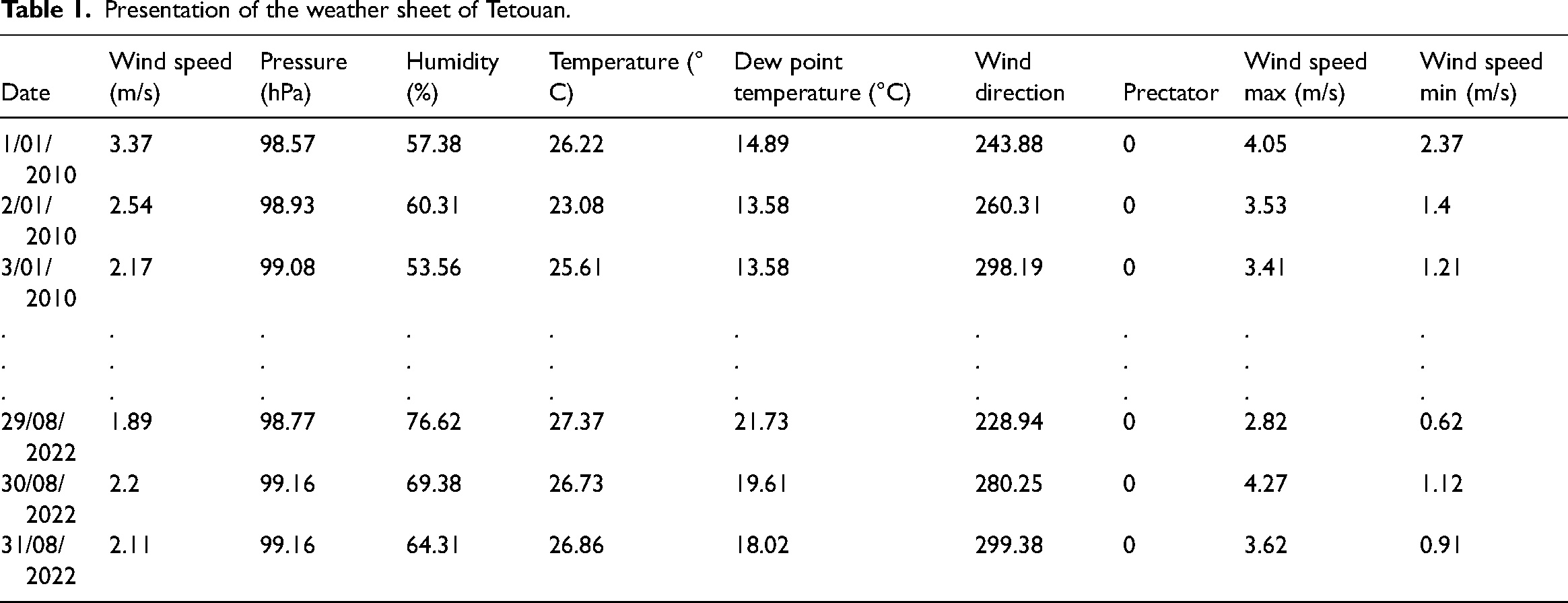
Our dataset includes daily records of wind speed, atmospheric pressure, wind temperature, dew temperature, humidity, minimum and maximum wind speed, and wind direction, along with precipitation data spanning 12 years, as shown in Table 1 (Masmoudi and Djebli, 2024).

Table 1.

Presentation of the weather sheet of Tetouan.

Date	Wind speed (m/s)	Pressure (hPa)	Humidity (%)	Temperature (°C)	Dew point temperature (°C)	Wind direction	Prectator	Wind speed max (m/s)	Wind speed min (m/s)
1/01/2010	3.37	98.57	57.38	26.22	14.89	243.88	0	4.05	2.37
2/01/2010	2.54	98.93	60.31	23.08	13.58	260.31	0	3.53	1.4
3/01/2010	2.17	99.08	53.56	25.61	13.58	298.19	0	3.41	1.21
.	.	.	.	.	.	.	.	.	.
.	.	.	.	.	.	.	.	.	.
.	.	.	.	.	.	.	.	.	.
29/08/2022	1.89	98.77	76.62	27.37	21.73	228.94	0	2.82	0.62
30/08/2022	2.2	99.16	69.38	26.73	19.61	280.25	0	4.27	1.12
31/08/2022	2.11	99.16	64.31	26.86	18.02	299.38	0	3.62	0.91

Data preprocessing and variables selection

Data preprocessing is essential for ensuring the accuracy of predictive models. We pre-processed the collected data using Excel by replacing all empty cells with zeros and removing non-numerical variables that were incompatible with MATLAB and could interfere with the learning process.

For variable selection, we calculated the correlation coefficient between each pair of variables using Excel. This step helped us eliminate redundant variables that provide similar information. For example, dew temperature and wind temperature had a correlation coefficient greater than 0.8, indicating they convey similar data. Removing such variables streamlined the model and improved its performance. The details of the correlation coefficient calculation (R) are discussed in our previous research (Masmoudi and Djebli, 2024).

The model inputs include seven variables: pressure, relative humidity, surface temperature, precipitation, wind direction, maximum wind speed, and minimum wind speed, all at time t. The output variable is the wind speed to be predicted at the same time (Masmoudi and Djebli, 2024).

Introduction to time-series forecasting

In time-series forecasting, future values are predicted using previous data that has been gathered over an extended period. This type of analysis is crucial for many applications, including financial market analysis, weather forecasting, and energy management (Kolambe and Arora, n.d.). Accurate time-series forecasting allows for better planning and decision-making, ultimately leading to more efficient and effective operations. In the context of wind speed prediction, accurate forecasts enable optimized wind energy production, grid stability, and efficient energy management (van der Merwe et al., n.d.).

Forecasting time-series data presents several challenges:

Nonlinearity: Time-series data, such as wind speed, can show nonlinear patterns that are challenging to describe using conventional linear techniques.

Noise: Time-series data may have random fluctuations and be noisy, making it difficult to see the underlying trends.

Temporal Dependencies: Current values in a time series often depend on past values, creating temporal dependencies that need to be accurately modeled.

Seasonality: There may be recurring patterns or cycles at specific intervals that must be accounted for.

Trend Analysis: Long-term patterns or shifts in the data must be identified and modeled.

Stationarity: Ensuring that the statistical properties of the time series remain constant over time can be challenging, especially with data that exhibit trends or seasonality (Ghazvini et al., 2024).

Understanding these challenges is essential for selecting appropriate forecasting models that can handle the intricate dependencies and persistent patterns observed in time-series data.

Forecasting models

In the following sections, we initially define both open-loop and closed-loop architectures for the NARX model. We will employ the open-loop configuration during the training phase, as it allows the model to utilize actual past values for prediction, thereby ensuring more accurate learning of the underlying data patterns. Based on the performance metrics obtained during this phase, (MAE), (MSE), and (RMSE), we will assess the model's accuracy and robustness. If the open-loop NARX model demonstrates satisfactory performance, we will then proceed to use the closed-loop configuration for multi-step-ahead predictions. Similarly, throughout training, the LSTM model's performance will be evaluated. The model that demonstrates the best performance in terms of these metrics will be selected for forecasting future values. Thus, the final decision on which model to use for future predictions will be based on the training phase results of both the NARX and LSTM models.

A- NARX Neural Network

The nonlinear autoregressive with exogenous inputs (NARX) model, is designed for time series prediction tasks with input and output delays (Song et al., 2021). It can be implemented in two main architectures: series-parallel architecture (open-loop) and parallel architecture (closed-loop) as mentioned in Figure 1 and the mathematical representation of these architectures is described by Equations (1) and (2) as follows (Boussaada et al., 2018).

Figure 1.

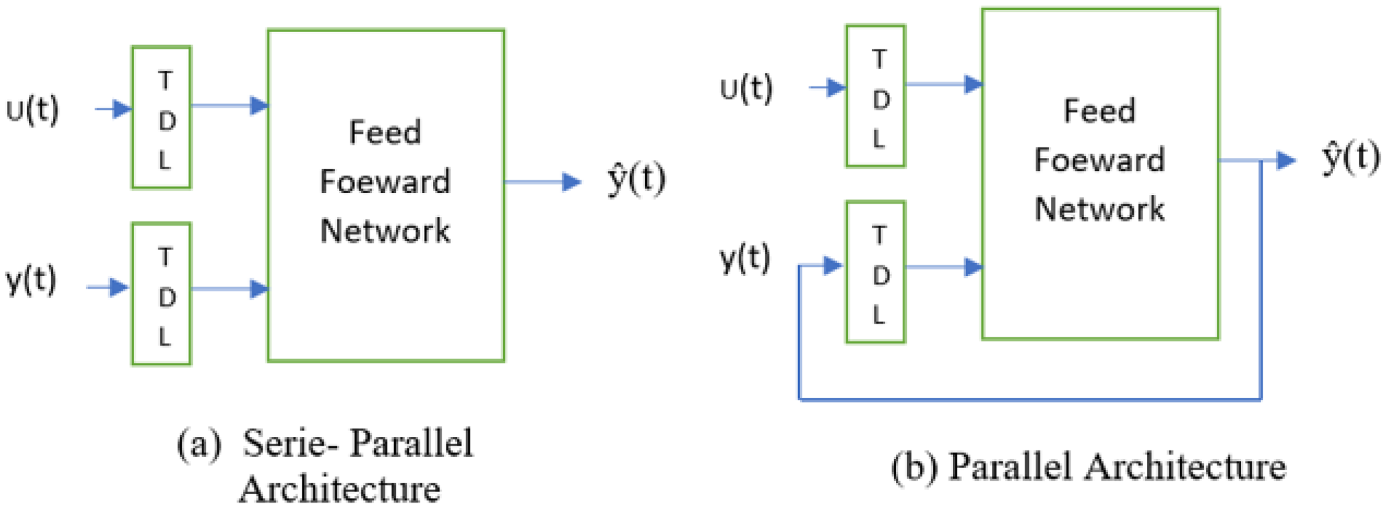
Narx neural network architectures.

The series-parallel architecture (open-loop) and parallel architecture (closed-loop) equations are shown as follows (Sadeghian Broujeny et al., 2023):

y (t) = f (y (t - 1), y (t - 2), \dots, y (t - d), u (t), u (t - 1), u (t - 2), \dots, u (t - q))

(1)

\hat{y} (t) = f (\hat{y} (t), \hat{y} (t - 2), \dots, \hat{y} (t - d), u (t), u (t - 1), u (t - 2), \dots, u (t - q))

(2)

Where:

y(t): The output at time (t).

ŷ(t): The predicted output at the time (t).

u(t): The input at time (t).

d: The number of past output delays.

q: The number of past input delays.

f be the activation function representing the relationship between the current output and past outputs, past inputs.

In open loop or series-parallel architecture, time series’ future values are estimated using its past values and the values of another external series, u(t). This architecture is particularly beneficial for training because it reduces the accumulation of prediction errors by providing the model with the true past outputs. This helps the model learn more accurately from the data. Additionally, the training is conducted using the Levenberg–Marquardt algorithm, which is frequently utilized in feed-forward networks, particularly when rapid training is required (Zuazo et al., 2021).

In the parallel (closed-loop) architecture the NARX network can make multi-step-ahead predictions if future exogenous inputs are available. This is achieved by using each one-step-ahead prediction as an input for the next prediction, iteratively continuing this process for the desired number of steps ahead (Raptodimos and Lazakis, 2020).

B- LSTM neural network

A specific type of RNN (recurrent neural network), long short-term memory networks (LSTMs), were created to solve the vanishing gradient issue that conventional RNNs encounter.

LSTMs introduce memory units and a gating mechanism, allowing them to retain information over extended periods and efficiently extract time series data's long-term dependencies.

On the other hand, weights in simple RNNs serve as long-term memory, gradually changing over training to encode general information about the training data. Additionally, they have transient activations that move from one node to the next that serve as short-term memory.

The construction of an LSTM model is shown in Figure 2. Typically, an LSTM model consists of four more layers: the forget gate (ft), the cell state (Ct), the input gate (it), and the output gate (ot). These layers interact uniquely to extract and generate information from the training data. Each parameter mentioned in the following paragraphs is defined by its meaning in this figure (Okut, 2021).

Cell state

Figure 2.

LSTM model diagram (Sood, n.d.).

The LSTM's memory is managed by the forgetting of old information (forget gate) and the addition of new information (input gate). Information travels through the LSTM with simple operations like multiplication and addition. If there are no interactions, the information remains unchanged. The LSTM block uses gates to add or remove information from the cell state, allowing only relevant information to pass through (Okut, 2021).

Forget gate

ft decides which data to retain from the cell state and which to discard from memory. The amount of historical data that should be retained is determined by using a sigmoid function to generate a value between 0 and 1, as indicated by Equation (3) (Li et al., 2023).

f t = σ (W f [h t - 1, x t] + b f)

(3)

The function calculates the elements that control the cell state and hidden state of the layer using the old output (ht - 1) at time t - 1 and the current input (Xt) at time t. The outcomes are [0,1], where 1 denotes “completely hold this” and 0 denotes “completely discard this” (Okut, 2021).

Input gate

Controls what new information is added to the cell state from the current input. A sigmoid activation function is used to generate the input values and convert information between 0 and 1. So, mathematically the input gate is given by Equation (4) below:

i t = σ (W i [h t - 1, x t] + b i)

(4)

Where:Next, a vector of new candidate value Ct, is created as shown in Equation (5) (Okut, 2021).

C t = \tanh (W c [h t - 1, x t] + b c)

(5)

Equation (6) describes how the values of the input state and cell candidate are combined to construct and update the cell state. The prior cell state (Ct - 1) is updated into the current cell state (Ct) using a linear combination of the input gate and forget gate. Once more, the forget gate (ft) determines the percentage of the old memory cell content (Ct - 1) that should be retained, while the input gate (it) controls how much fresh data should be considered via the candidate (Ct).

The updated equation that results from using the same pointwise multiplication (⨀ = Hamard product) is as follows:

C t = f t ⊙ C t + i t ⊙ C \tilde{t}

(6)

Output gate

At each time step, the Output Gate (ot) controls which data from the updated cell state (Ct) is made available as output. In essence, it determines at each step the value of the subsequent concealed state. Tanh function is used to calculate the hidden state and generate predictions, while a sigmoid function is used to control this choice. This process is described by Equations (7), (8), and (9) (Okut, 2021).

o t = (W o (h t - 1, x t ⊙ b o))

(7)

h t = o t ⊙ t a n h C t

(8)

\hat{y} t = (W y h t + b y)

(9)

Methods and techniques related to machine learning

Data rescaling

Data rescaling is significant because it can enhance machine learning models’ training stability and performance. By ensuring that features are on a similar scale, rescaling can enhance the convergence of algorithms and prevent certain features from dominating the learning process due to their larger magnitude. Standardization is the technique used for this study to rescale the data set and make the preprocessing easier for the machine-learning methods.

Standardization involves setting the mean, µ, of the feature to 0 and ensuring that all feature values fall within one standard deviation, σ. One common standardization technique is the Standard Scaler, z, given by Equation (10) below (Eren, n.d.).

z = \frac{x i - μ}{σ}

(10)

Data augmentation, cross-validation, and dropout

To ensure the robustness of the models, we utilized a larger dataset spanning 12 years compared to previous studies that used only 5 years. The model performs better as a result of the increased data volume because it provides a more thorough description of the wind speed patterns, which enhances generalization and prediction accuracy.

Moreover, cross-validation techniques were implemented to evaluate the performance of the models. Specifically, k-fold cross-validation was used for the NARX neural network, where k = 5 subsets (folds) were created from the dataset. After training on k - 1 folds, the models were tested on the remaining folds. Every fold was utilized as the test set once during the k repetitions of this process. A more accurate estimate of the model's performance was then obtained by averaging the results. In order to minimize the possibility of overfitting and produce a more reliable assessment, cross-validation makes sure that the models are evaluated on several subsets of the data (Eren, n.d.).

For the LSTM neural network, we employed dropout, a regularization technique designed to prevent overfitting and improve generalization. Dropout involves randomly removing (or “dropping out”) units, both hidden and visible, along with their connections during training. This process is performed independently for each hidden unit and each training instance. Typically, each unit is retained with a fixed probability (p), although this value can be fine-tuned using a validation set (Salehin and Kang, 2023). In this study, we chose (p = 2). By doing this, a “thinned” version of the neural network is created for each training iteration, which helps ensure that the model does not become overly reliant on specific neurons and promotes better generalization.

The choice of k-fold cross-validation for the NARX neural network and dropout for the LSTM neural network is justified by the specific characteristics and requirements of these models. The NARX model benefits from cross-validation due to its dependency on temporal sequences, where different subsets of the data can provide varied and comprehensive training scenarios.. Conversely, dropout is necessary for the LSTM model, which is well-known for its capacity to manage long- term dependencies in data, in order to keep the model from growing overly complicated and overfitting to the training set.

Data splitting

Data splitting, in which the dataset is separated into two distinct sets, training, and testing, is a commonly used technique for model validation (Joseph, 2022). In this study, the dataset was randomly split into 80% for training, 10% for validation, and 10% for testing. Allocating 80% of the data for training ensures that the model has a sufficiently large dataset to learn from, capturing more patterns and relationships. The 10% reserved for validation allows for independent tuning of hyperparameters and evaluation during training, minimizing bias. The remaining 10% is used for testing, providing a final, unbiased evaluation of the model's performance on unseen data.

Machine learning metrics

This study will use three different metrics to thoroughly evaluate the performance of the machine learning method:

MAE is a commonly used metric that calculates the mean absolute deviation between the values that were expected and those that were obtained. It is calculated by averaging the absolute differences for each observation in the time series as given by Equation (11). MAE is especially useful for understanding the size of prediction errors without considering their direction (Kolambe and Arora, n.d.).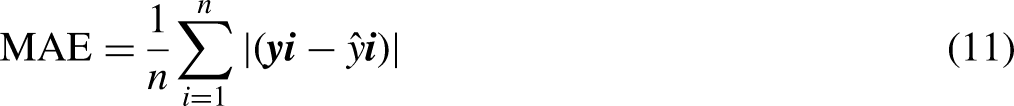

MAE = \frac{1}{n} \sum_{i = 1}^{n} | (y i - \hat{y} i) |

(11)

Where:

n is the number of observations.

yi is the actual value at time i.

ŷi is the predicted value at the time i (Faraji et al., 2023).

One often used statistic for evaluating regression models is mean squared error (MSE). It calculates the mean of the squared discrepancies between the actual and anticipated values. An MSE of 0 means that the model's predictions and the actual values match perfectly, with a lower MSE denoting greater performance (Li et al., 2023).

The formula for calculating MSE is given by Equation (12):

MSE = \frac{1}{n} \sum_{i = 1}^{n} {(y i - \hat{y} i)}^{2}

(12)

Where:

n is the number of observations.

yi is the actual value at time i.

ŷi is the predicted value at the time i (Faraji et al., 2023).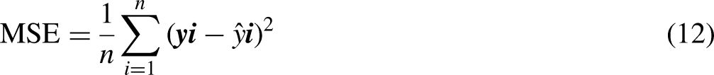

RMSE, the root mean squared error, is derived from MSE and serves as a common metric in various fields. It offers a practical advantage by presenting errors in the original units of the data, making it more interpretable for assessing forecast accuracy. Additionally, RMSE generates smaller values compared to MSE, enhancing its utility in comparing the performance of different models or techniques (Eren, n.d.).

The formula for calculating RMSE is given by Equation (13):

RMSE = \sqrt{\frac{1}{n} \sum_{i = 1}^{n} {(y i - \hat{y} i)}^{2}}

Where:

n is the number of observations.

yi is the actual value at time i.

ŷi is the predicted value at the time i (Faraji et al., 2023).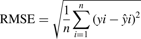

Results and discussion

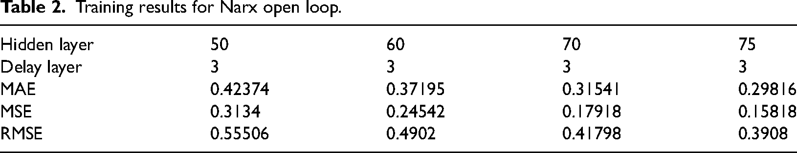
Tables 2 and 3 present respectively the performance metrics (MAE, MSE, RMSE) for the NARX and LSTM models with varying numbers of neurons. For the NARX model, configurations with 50, 60, 70, and 75 neurons were tested, while the LSTM model was evaluated with 50, 100, 200, and 300 neurons.

Table 2.

Training results for Narx open loop.

Hidden layer	50	60	70	75
Delay layer	3	3	3	3
MAE	0.42374	0.37195	0.31541	0.29816
MSE	0.3134	0.24542	0.17918	0.15818
RMSE	0.55506	0.4902	0.41798	0.3908

Table 3.

Results for LSTM during the training phase.

HiddenUnites	50	100	200	300
SequenceInputLayer	1	1	1	1
FullyConnectedLayer	1	1	1	1
MAE	0.31249	0.22625	0.19388	0.18855
MSE	0.1785	0.1090	0.0733	0.0666
RMSE	0.42248	0.33014	0.27072	0.25808

The choice of a delay of 1:3 in the NARX model was based on the aim of capturing sufficient historical information while balancing computational efficiency. This configuration provides a compromise between capturing temporal dependencies and managing model complexity. The delay setting was chosen after evaluating various configurations to ensure optimal performance for the specific forecasting task.

When using the same number of neurons (50) for both models, the LSTM model outperformed the NARX model, likely due to its enhanced capability to capture complex data patterns.

Both models exhibited enhanced performance with an increase in the number of neurons. Specifically, the NARX model achieved optimal results with 75 neurons, showing the lowest MAE of 0.29816, MSE of 0.15818, and RMSE of 0.3908. In contrast, the LSTM model continued to show improvement as the number of neurons increased, reaching its peak performance with 300 neurons, where it achieved the lowest MAE of 0.18855, MSE of 0.0666, and RMSE of 0.25808. Overall, the LSTM model consistently demonstrated superior performance across all metrics compared to the NARX model as shown in Table 3.

Figure 3.

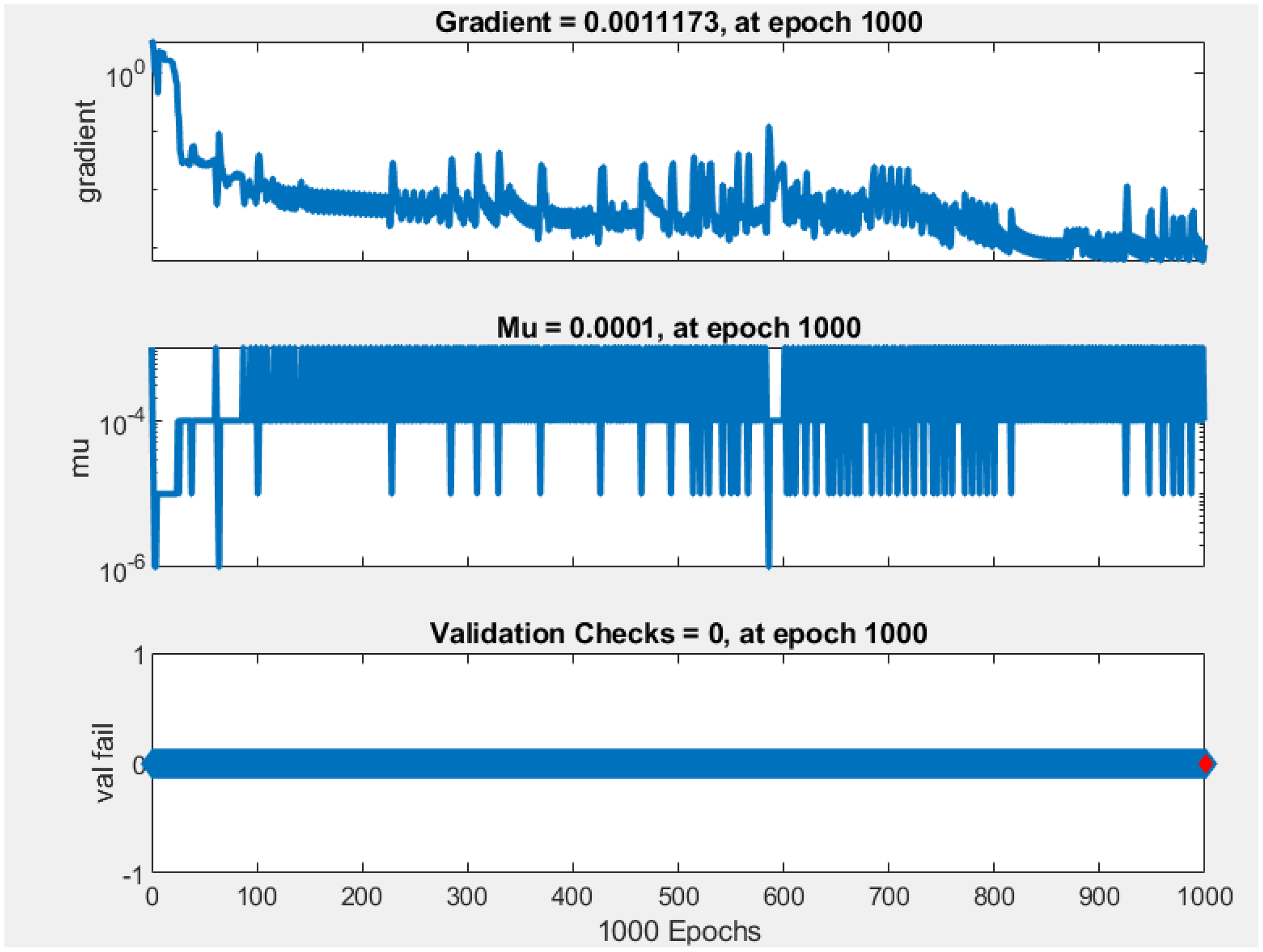
NARX training phase.

To further understand these results, we will examine the regression plots and training dynamics for both models, specifically for the 300-neuron LSTM configuration and the 75-neuron NARX configuration. This analysis will help us determine if the observed performance metrics align with the models’ training behaviors and predictive accuracy.

The NARX training process is visualized in Figure 3 through three plots: gradient, mu, and validation checks. The gradient plot shows a decrease and fluctuation over epochs, stabilizing at a small value of 0.0011173 by epoch 1000, suggesting potential vanishing gradient issues that could hinder effective learning. The mu plot indicates stabilization at 0.0001, reflecting a steady training adjustment factor. However, the validation checks remained constant at 0 throughout training, which contrasts with typical variations observed in related works (Chelliah and Benadict, Bensiger, 2015). This constant value raises concerns about potential issues with the validation process or model evaluation, possibly indicating that the model's generalization performance was not accurately monitored.

Figure 4.

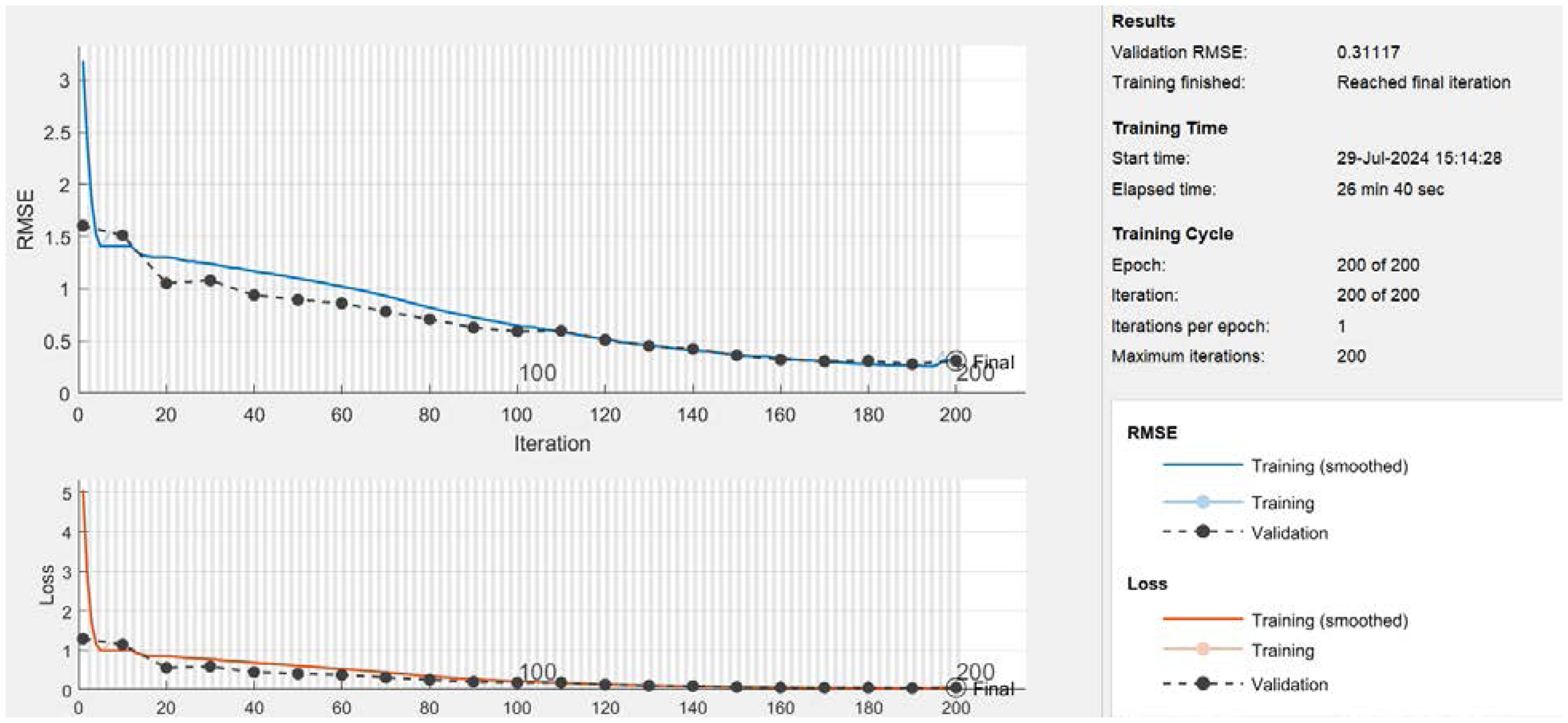
The LSTM training process.

The training time of 14 minutes for the NARX model is relatively short. While this quick training could indicate efficient processing, it may also suggest that the model might not be fully learning the underlying patterns in the data. In some cases, short training times can be a sign of overfitting, especially if the model is too simple to capture complex patterns or if the validation performance is not properly monitored.

The LSTM training process is illustrated in Figure 4 above through two plots: RMSE and loss over epochs. The loss plot shows a rapid decline, nearing zero within 100 iterations, indicating effective minimization of the error function and a strong fit to the training data. The RMSE plot reveals a more gradual decrease, continuing to improve beyond 100 epochs and eventually stabilizing. This gradual reduction in RMSE highlights its sensitivity to the scale of errors and provides a more interpretable measure of model performance. The training time of 26 minutes and 40 seconds aligns with the complexity of the LSTM model and dataset size, reflecting efficient learning and adaptation. These metrics show that the LSTM model with 300 neurons achieved significant improvements in reducing training error and prediction discrepancies.

We evaluated the performance of both models using regression plots, which illustrate the relationship between predicted and actual values as shown in Figures 5 and 6, respectively. The Pearson correlation coefficient (R) values are as follows:

NARX Model (R = 0.88345)

LSTM Model (R = 0.9851).

Figure 5.

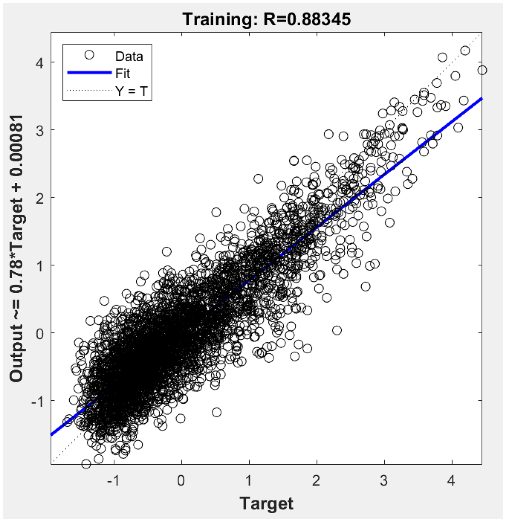
The regression plot for NARX neural network.

Figure 6.

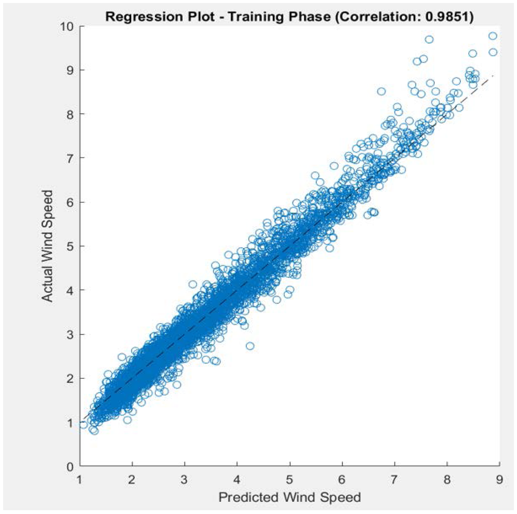
The regression plot for LSTM.

The degree and direction of the linear relationship between the predicted and actual values are measured by the (R) value (Pokhrel et al., 2024). With higher values indicating better model performance, the regression analysis shows that the LSTM model with 300 neurons significantly outperforms the NARX model with 75 neurons suggesting superior prediction accuracy. Despite using 5-fold cross-validation, the NARX model may still suffer from overfitting. In contrast, the LSTM model benefits from dropout regularization, which helps mitigate overfitting and enhances its predictive performance.

The LSTM model's good forecasting performance is demonstrated by the results of Table 4 and Figure 7, which show that the model's forecasts for August match up well with actual wind speeds. For example, the actual result of 5.14 differs by only 0.02 from the anticipated value of 5.12. These slight variations demonstrate how accurately the model captures greater wind speeds.

Figure 7.

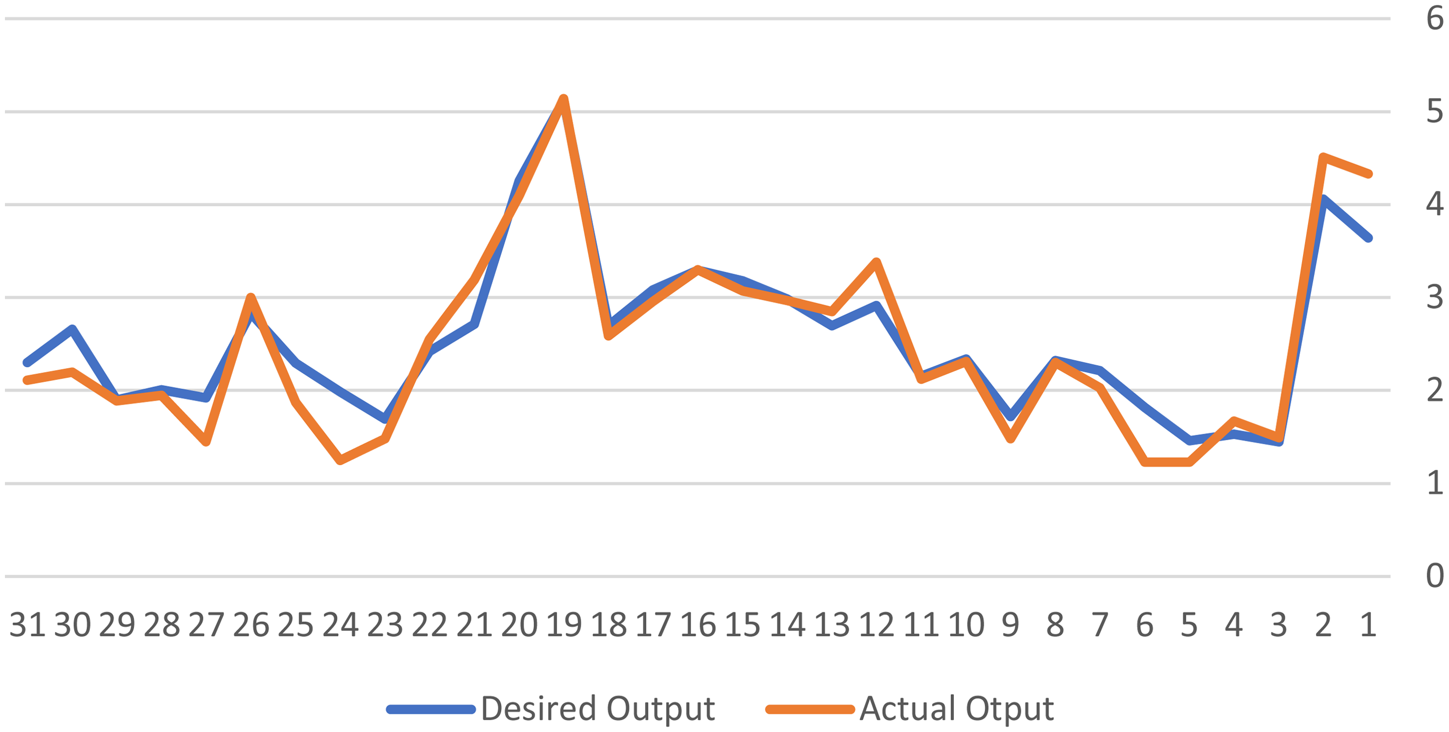
LSTM forecast results for 31 days of August.

Table 4.

Prediction of August 2022 using LSTM with 300 neurons.

Actual wind speed values	Forecasted find speed values
4.3300	3.6410818
4.5100	4.0587368
1.4900	1.4475604
1.6700	1.5291469
1.2300	1.4572320
1.2300	1.8150432
2.0300	2.2125182
2.3000	2.3244367
1.4800	1.7225929
2.3100	2.3386757
2.1200	2.1522307
3.3800	2.9164858
2.8500	2.6985722
2.9700	2.9823675
3.0700	3.1799455
3.3000	3.2936971
2.9600	3.0821483
2.5900	2.6973069
5.1400	5.1203632
4.1000	4.2562437
3.1900	2.7120163
2.5500	2.4199295
1.4800	1.6918812
1.2500	1.9853381
1.8700	2.2979734
3	2.8348503
1.4500	1.9222634
1.9500	2.0056181
1.8900	1.8971617
2.2000	2.6563230
2.1100	2.2997479

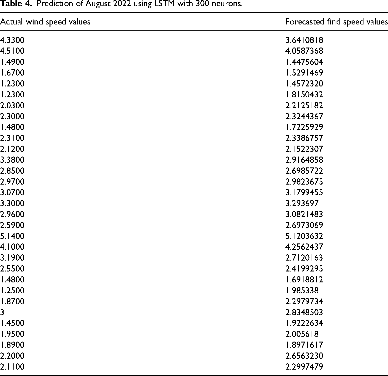
The model also performs well with lower wind speeds. For example, a prediction of 1.45 is close to the actual 1.49, with a difference of 0.04. Another close match is a prediction of 1.99 compared to the actual 1.87, showing a difference of 0.12. However, there are some notable discrepancies, such as a forecast of 3.64 compared to the actual 4.33 (a difference of 0.69) and 1.69 compared to the actual 1.23 (a difference of 0.46). These larger deviations indicate areas where the model needs to be improved for more precise predictions.

The enhanced predictive accuracy of the LSTM model has important implications for energy optimization. In the context of wind energy production, precise wind speed forecasts are crucial for optimizing turbine operation and integrating energy into the grid efficiently. With better prediction capabilities, energy providers can more accurately anticipate wind conditions, adjust turbine settings to maximize energy output and improve grid management. For instance, more reliable forecasts enable better scheduling of energy storage and reduce dependency on backup power sources. As a result, the adoption of the LSTM model could lead to significant improvements in energy efficiency and sustainability, ultimately benefiting both energy producers and consumers.

Delimitations of the study

When considering the findings of this study, it is important to recognize several limitations:

Data Source: The study relied exclusively on the NASA POWER dataset for meteorological data. While this dataset offers valuable information, using only one source may introduce biases and inaccuracies. The spatial and temporal resolution of the NASA POWER data might not capture localized wind patterns specific to Tetouan City (Vallejo Díaz et al., 2024). Additionally, the data comes from atmospheric models and satellite observations, which can have measurement errors and modeling uncertainties that affect the precision of predictions.

Preprocessing: Limitations exist in the preprocessing steps. Non-numerical variables were removed for compatibility with the model, and missing values were replaced with zeros. This could introduce artificial patterns or biases. Standardization was used to stabilize the training process and improve model performance, but it might not fully address underlying data quality issues (Eren, n.d.).

Hyperparameter Optimization: The study used a Random Search for hyperparameter optimization, but exploring a larger search space or using advanced techniques like Bayesian Optimization could potentially improve model performance. Time and computational constraints limited the use of more sophisticated methods.

Dropout Regularization: Dropout was employed as a regularization technique in the LSTM neural network to prevent overfitting. While dropout helps to reduce overfitting by randomly dropping units during training, it may not fully address other potential model weaknesses or data issues.

k-Fold Cross-Validation for NARX: The NARX model was evaluated using 5-fold cross- validation to assess its performance and reduce overfitting. While this method provides a robust evaluation by testing the model on different subsets of the data, it may still limit the generalizability of the findings compared to other validation techniques. Additionally, the use of 5-fold cross- validation may introduce variability in performance metrics depending on the data splits.

Time Frame and Generalizability: The study used data from 2010 to 2022, providing a comprehensive dataset. However, relying solely on this data source might still limit the generalizability of the findings. While k-fold cross-validation was implemented to assess model performance and reduce overfitting, incorporating additional data sources and validation methods could strengthen the robustness of the results.

Future studies could overcome these limitations by integrating ground-based meteorological data from local weather stations and cross-referencing it with other sources. This would help validate and enhance the NASA POWER data, improving the accuracy and reliability of wind speed predictions for Tetouan City. By acknowledging and addressing these limitations, future studies can provide a more thorough and reliable analysis.

Conclusion

In order to determine how well the LSTM and NARX models performed in Tetouan City in predicting wind speed, this study evaluated their accuracy and usefulness for forecasting in the future. The LSTM model was found to be the better option after using the performance measures MAE, MSE, and RMSE and assessing the R-value during the training phase. The LSTM model successfully handled the complexity of Tetouan's meteorological data, as evidenced by its high R-value of 0.9851 and consistent accuracy. Its increased robustness and dependability for predicting future wind speeds are demonstrated by its decreased error rates throughout the assessed measures. Because of the LSTM model's better training results and predicted accuracy, it was chosen for use in subsequent forecasts.

In contrast, the NARX model performed less well in comparison, despite its value, with greater error rates and a lower R-value. Consequently, it is utilized only in its open-loop form, not for future forecasting.

In conclusion, the improved accuracy and performance of the LSTM model support its application for Tetouan City's upcoming wind speed forecasts, providing a more dependable wind energy management tool. To further improve and validate these models, future research could profit from investigating new data sources and sophisticated approaches.

Footnotes

Authors’ contributions

All authors contributed to the study's conception and design. Material preparation, data collection, and analysis were performed by Wissal Masmoudi, Abdelouahed Djebli, and Faouzi Moussaoui. The first draft of the manuscript was written by Wissal Masmoudi and all authors commented on previous versions of the manuscript. All authors read and approved the final manuscript.

Declaration of conflicting interests

The authors declared no potential conflicts of interest with respect to the research, authorship, and/or publication of this article.

Ethical approval

This study does not contain any studies with human or animal subjects performed by any of the authors.

Funding

The authors received no financial support for the research, authorship, and/or publication of this article.

ORCID iD

Wissal Masmoudi

References

Boussaada

Curea

Remaci

, et al. (2018) A nonlinear autoregressive exogenous (NARX) neural network model for the prediction of the daily direct solar radiation. Energies 11(3): 620.

Chelliah

Benadict Bensiger

(2015) Prediction of failure load in glass/epoxy laminates from acoustic emission monitoring using artificial neural network. Unpublished. Available at: http://rgdoi.net/10.13140/RG.2.1.1247.0887 (accessed 28 August 2024).

Eren

(2023.) Comparative analysis of machine learning methods for predicting property prices and sale velocities in the real estate industry.

Faraji

Shooshtari

El-Hag

(2023) Stacked ensemble regression model for prediction of furan. Energies 16(22): 7656.

Ghazvini

Sharef

Sidi

(2024) Prediction of course grades in computer science higher education program via a combination of loss functions in LSTM model. IEEE Access: 1–1.

Joseph

(2022) Optimal ratio for data splitting. Statistical Analysis and Data Mining: The ASA Data Science Journal 15(4): 531–538.

Kharbouch

(2017) Énergies éolienne, énergies solaire thermique, énergies photovoltaïque.

Kolambe

Arora

(2024) Forecasting the future: A comprehensive review of time series prediction techniques.575-586

Shen

, et al. (2023) Exploring time series models for wind speed forecasting: A comparative analysis. Energies 16(23): 7785.

10.

Masmoudi

Djebli

(2024) Forecast of wind speed based on MLP network model using Levenberg Marquardt and gradient descent algorithms in Tetouan City, Northern Morocco. Wind Engineering: 0309524X231215812.

11.

Okut

(2021) Deep learning for subtyping and prediction of diseases: Long-short term memory. In: Luigi Mazzeo

Spagnolo

(eds) Deep Learning Applications. IntechOpen, pp. 1–25. Available at: https://www.intechopen.com/books/deep-learning-applications/deep-learning-for-subtyping-and-prediction-of-diseases-long-short-term- memory (accessed 8 February 2024).

12.

Pokhrel

Dahal

Rimal

, et al. (2024) Deep-SDM: A unified computational framework for sequential data modeling using deep learning models. Software 3(1): 47–61.

13.

Raptodimos

Lazakis

(2020) Application of NARX neural network for predicting marine engine performance parameters. Ships and Offshore Structures 15(4): 443–452.

14.

Sadeghian Broujeny

Ben Ayed

Matalah

(2023) Energy consumption forecasting in a university office by artificial intelligence techniques: An analysis of the exogenous data effect on the modeling. Energies 16(10): 4065.

15.

Salehin

Kang

D-K

(2023) A review on dropout regularization approaches for deep neural networks within the scholarly domain. Electronics 12(14): 3106.

16.

Serikov

Zhetpisbayeva

Mirzakulova

, et al. (2021) Application of the NARX neural network for predicting a one-dimensional time series. Eastern-European Journal of Enterprise Technologies 5(4 (113)): 12–19.

17.

Song

Sun

Zhang

, et al. (2021) Prediction of road network traffic state using the NARX neural network. Journal of Advanced Transportation 2021: 1–17.

18.

Sood

(n.d.) Long short-term memory.

19.

Zheng

(2023) A combined model based on secondary decomposition technique and grey wolf optimizer for short-term wind power forecasting. Frontiers in Energy Research 11: 1078751.

20.

Vallejo Díaz

Herrera Moya

Garabitos Lara

, et al. (2024) Assessment of urban wind potential and the stakeholders involved in energy decision-making. Sustainability 16(4): 1362.

21.

van der Merwe

du Plessis

Rix

(2023) WIND POWER FORECASTING: A REVIEW. November 2023.

22.

Zejli

Benchrifa

(2010) L’énergie éolienne: de la source d’énergie renouvelable la moins prometteuse à la plus convoitée. Revue des Energies Renouvelables SMEE'10 Bou Ismail Tipaza (2010): 359–368.

23.

Zuazo

Boussaada

Aginako

, et al. (2021) Short-term load forecasting of building electricity consumption using NARX neural networks model. In: 2021 6th International Conference on Smart and Sustainable Technologies (SpliTech), Bol and Split, Croatia, 8 September 2021, pp. 1–6. IEEE. Available at: https://ieeexplore.ieee.org/document/9566440/ (accessed 29 August 2024).

Evaluating LSTM and NARX neural networks for wind speed forecasting and energy optimization in Tetouan,Northern Morocco

Abstract

Keywords

Introduction

Materials and methods of the research

Data collection

Data preprocessing and variables selection

Introduction to time-series forecasting

Forecasting models

Methods and techniques related to machine learning

Data rescaling

Data augmentation, cross-validation, and dropout

Data splitting

Machine learning metrics

Results and discussion

Delimitations of the study

Conclusion

Footnotes

Authors’ contributions

Declaration of conflicting interests

Ethical approval

Funding

ORCID iD

References