
Abstract
Responsible, efficient, and environmentally conscious energy consumption practices are increasingly essential for ensuring the reliability of the modern electricity grid. This study focuses on leveraging time series analysis to improve forecasting accuracy, crucial for various application domains where real-world time series data often exhibit complex, non-linear patterns. Our approach advocates for utilizing long short-term memory (LSTM) and bidirectional long short-term memory (Bi-LSTM) models for precise time series forecasting. To ensure a fair evaluation, we compare the performance of our proposed approach with traditional neural networks, time-series forecasting methods, and conventional decline curves. Additionally, individual models based on LSTM, Bi-LSTM, and other machine learning methods are implemented for a comprehensive assessment. Experimental results consistently demonstrate that our proposed model outperforms all benchmarking methods in terms of mean absolute error (MAE) across most datasets. Addressing the imbalance between activations by consumer and prosumer groups, our predictions show superior performance compared to several traditional forecasting methods, such as the autoregressive integrated moving average (ARIMA) model and seasonal autoregressive integrated moving average (SARIMA) model. Specifically, the root mean square error (RMSE) of Bi-LSTM is 5.35%, 46.08%, and 50.6% lower than LSTM, ARIMA, and SARIMA, respectively, on the May test data.
Keywords
Introduction
Forecasting energy consumption is a significant and complex undertaking within both industry and academia. Precise predictions of energy consumption offer valuable insights for efficiently allocating energy resources (Liu et al., 2018), devising energy-saving strategies (Han et al., 2008), and enhancing overall energy system performance. Additionally, accurate energy predictions assist managers in conducting market research management and facilitating economic development (Pao, 2009). From an academic perspective, the advancements in energy consumption prediction can be extended to forecasting other time series, including but not limited to traffic flow (Fu et al., 2017), weather patterns (Rasp and Lerch, 2018), temperature trends (Zhang et al., 2017), stock market behavior, and solar radiation levels.
Different methods for forecasting time series have been developed in previous research (Alizadegan et al., 2024), falling into categories like statistical approaches, computational intelligence, and a blend of the two. Among the statistical techniques, autoregressive integrated moving average (ARIMA) is widely used for modeling linear time series (Kumaresan and Ganeshkumar, 2020). However, real-world time series often demonstrate non-linear characteristics (Shaeri et al., 2022), making it essential to employ non-linear modeling techniques (Panigrahi and Behera, 2017; Shaeri et al., 2022). Computational intelligence techniques, such as feedforward neural networks (NNs) (Mengesha et al., 2022; Shaeri et al., 2022), provide a means to effectively capture and model these non-linear patterns.
While conventional computational intelligence methods like feedforward neural networks can effectively model intricate patterns among samples, they struggle to capture the long-term dependencies present in time series data. As a result, recurrent neural networks (RNNs), a specialized type of artificial neural networks, have been introduced as a viable alternative for accurate time series forecasting (Chen et al., 2018).
Even though RNNs are adept at retaining sequential information, they encounter challenges such as the vanishing gradient problem, making their training difficult (Parmezan et al., 2019). Consequently, a solution has been found in the form of long short-term memory (LSTM) networks, which serve as an extension of RNNs. LSTMs have been developed to overcome the limitations of RNNs and have proven successful in processing sequence data, including applications such as natural language processing (NLP) and speech recognition (Fischer and Krauss, 2018).
Given the significant advancements observed in the aforementioned application domains and the crucial importance of precise time series forecasting in this context (Abbasimehr and Paki, 2022), the present study conducts a comparison of various time series forecasting models for predicting energy consumption prediction. The evaluated methods encompass both statistical (persistent) approaches and those rooted in artificial intelligence. The statistical models utilized in this study fall under the category of persistence models, including Autoregressive Moving Average (ARMA), ARIMA, and Seasonal AutoRegressive Integrated Moving Average (SARIMA). Additionally, six different types of neural network (NN) models are considered: bidirectional long short-term memory (Bi-LSTM), LSTM (Alizadegan et al., 2024), fuzzy C-mean clustering, multi-layer perceptron (MLP) and feedforward neural networks (Sharadga et al., 2020).
This study addresses a gap in existing literature on energy consumption forecasting by comparing traditional statistical models (ARIMA, SARIMA) and advanced deep learning approaches (LSTM, Bi-LSTM). Traditional models often fail to capture the non-linear, dynamic patterns of energy consumption data influenced by variables like weather and socio-economic factors. This research aims to provide empirical evidence of the relative strengths and weaknesses of these methodologies for more accurate predictions. For this purpose, we contribute to the field of energy consumption forecasting through a systematic evaluation of LSTM and Bi-LSTM deep learning models against traditional ARIMA and SARIMA methods.
This study is guided by the following research questions: How do deep learning models like LSTM and Bi-LSTM compare to traditional statistical methods such as ARIMA and SARIMA in forecasting energy consumption? What are the strengths and weaknesses of each approach in accurately predicting complex, non-linear patterns in time series data?
Additionally, we hypothesize that incorporating temporal features enhances the predictive accuracy of LSTM and Bi-LSTM models for energy consumption forecasting. We also propose that the performance of these models remains consistent across various datasets, regardless of the scale and type of energy consumption patterns they represent.
In our comparative analysis of energy consumption prediction models, the utilization of LSTM and Bi-LSTM networks consistently demonstrated superior predictive performance over traditional statistical models such as ARIMA and SARIMA. LSTM and Bi-LSTM models exhibited enhanced accuracy in capturing intricate, non-linear patterns and prolonged dependencies within the data, as evidenced by notably lower mean absolute error (MAE) and root mean square error (RMSE) metrics. Particularly noteworthy was Bi-LSTM's ability to leverage bidirectional processing, resulting in the highest accuracy among the models tested. In contrast, ARIMA and SARIMA, while effective in modeling linear trends and seasonal variations, struggled to adequately handle the non-linear dynamics inherent in energy consumption data, thereby yielding higher prediction errors compared to the deep learning approaches. This underscores the superior capability of LSTM and Bi-LSTM networks in addressing the complexities and nuances present in real-world energy consumption forecasting tasks.
While existing literature has extensively discussed individual methodologies, there is a clear need for comprehensive comparative analyses to quantitatively assess the effectiveness of these models in capturing complex temporal patterns and enhancing forecasting accuracy. This comparative study aims to provide empirical evidence and insights that can guide decision-making in energy management and inform future advancements in predictive modeling techniques. The results of our study are compared with the recent publish papers in Web of Science (WoS) in section of “Results and Discussion” . In the “Methodology” section, we detail the approaches and frameworks utilized to investigate our research questions. Following this, the “Results and Discussion” section presents the empirical findings and their interpretations. Finally, the “Conclusion” section synthesizes these findings, discusses their implications, and suggests avenues for future research.
Related work
In recent years, RNNs have gained considerable traction in the realm of time series forecasting due to their inherent suitability for sequence modeling tasks. The effectiveness of RNNs, particularly the LSTM network, has been validated in several recent forecasting studies (Abbasimehr et al., 2020; Fischer and Krauss, 2018; Gundu and Simon, 2021; Kulshrestha et al., 2020; Law et al., 2019) For instance, Gundu and Simon (Gundu and Simon, 2021) proposed an LSTM model for electricity price forecasting, leveraging particle swarm optimization (PSO). Abbasimehr et al. (Abbasimehr et al., 2020) developed an optimized stacked LSTM model for demand forecasting in a furniture company, surpassing conventional benchmark models. Similarly, Fischer and Krauss (Fischer and Krauss, 2018) investigated LSTM networks’ performance in financial market forecasting, demonstrating their superiority over standard methods. Law et al. (Law et al., 2019) proposed a deep learning framework applied to tourism demand forecasting. In a related study, Kulshrestha et al. (Kulshrestha et al., 2020) presented a combined model integrating bidirectional LSTM and Bayesian optimization (BO) for tourism demand forecasting, showing improved performance compared to popular methods such as support vector regression (SVR), radial basis function neural networks (RBFNN), and autoregressive distributed lag model (ADLM)(Hosseini Rad et al., 2022; Ilani and Khoshnevisan, 2021, 2022). In another study compared two deep learning models, LSTM and Bi-directional LSTM (Bi-LSTM), for short-term univariate electric consumption forecasting across diverse datasets. Statistical evidence, including Friedman's test, indicates that Bi-LSTM significantly outperforms LSTM, demonstrating its robustness across different scales of electric power consumption (da Silva and de Moura Meneses, 2023).
Moreover, various models, including neural networks and decomposition techniques, have been developed to forecast solar irradiance. The WPD-based model achieved the lowest RMSE and MAE for Indian locations (Singla et al., 2023a). A hybrid RLMD Bi-LSTM model integrating RLMD and bidirectional LSTM significantly improved RMSE and MAE, outperforming traditional and RLMD-based models for short-term forecasts in Hisar and Jaipur (Singla et al., 2023b). A dual decomposition-based error correction model using CEEMDAN and VMD with bidirectional LSTM networks achieved lower RMSE and MAPE, validated by statistical tests, demonstrating robustness across multiple locations (Singla et al., 2022a).
Methodology
Predicting time series data that exhibits chaos, uncertainty, randomness, periodicity and nonlinearity is a significant challenge. This section presents the proposed framework for accurately predicting long-term energy consumption, with a specific focus on addressing distinct periodic patterns. The methodologies utilized are detailed below.
ARIMA and SARIMA
The ARIMA model proves valuable in time series forecasting by leveraging past values in the series. Accurate forecasting holds significance for cost saving measures, effective planning and production activities. When forecasting future values using historical data from a time series, it's known as univariate time series forecasting. On the other hand, if the series isn't utilized for prediction, it's termed as multivariate time series forecasting. ARIMA is proficient in predicting future values based on its own historical data, integrating lagged values and forecast error lags.
The ARIMA model comprises three key components:

The utilized combination involves a linear combination of lags, with the primary objective being the identification of appropriate values for p, d, and q. The selection of the minimum difference d is crucial, and it should be chosen based on achieving zero autocorrelation (AC). The determination of p is associated with the order of the autoregressive (AR) component, which should equal the lags in the partial autocorrelation (PAC) surpassing the set significance threshold. PAC represents a conditional correlation.
Equation (2) demonstrates the PAC, where y represents the response variable and x1, x2, and x3 denote predictor variables. More precisely, Eq. (2) delineates the PAC between y and x3, computed as the correlation between the regression residuals of y on x1 and x2, and the residuals of x3 on x1 and x2.


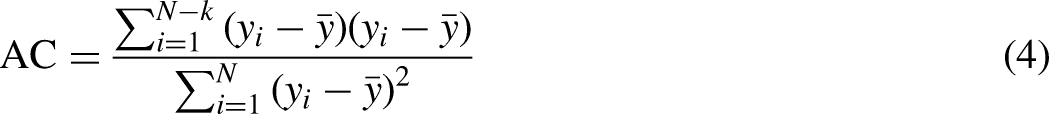
The lag is represented by k.
N represents the complete series value.
In cases where there is a need to account for seasonal patterns in the time series, a seasonal term is incorporated into the ARIMA model. This results in the seasonal ARIMA model, denoted as SARIMA, as it notation is provided below:

Recurrent neural network
RNNs are a specialized class of neural networks designed to recognize patterns in sequences of data, such as time series or natural language. Among the various forms of RNNs, LSTM and Bi-LSTM stand out due to their capability to retain and utilize information over extended sequences, making them highly effective for tasks that involve sequential data prediction.
Long short-term memory
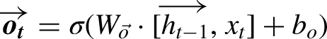
LSTMs are designed to address the vanishing gradient problem inherent in traditional RNNs by using unique memory blocks called cells, which include three primary gates: input, forget, and output gates. These gates control the flow of information through the cell.
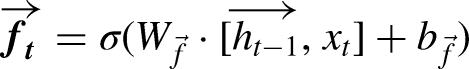
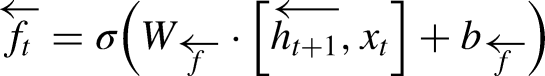
The forget gate determines which information from the previous cell state should be discarded, and is described by the equation: (Singla et al., 2022c):

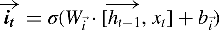
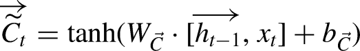
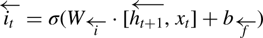
The input gate updates the cell state with new information, using the equations:


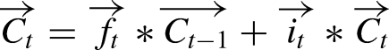
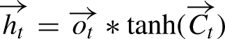
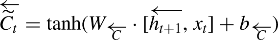
The cell state is then updated by combining the previous cell state and the new candidate cell state:
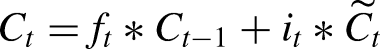

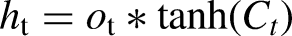
These equations show how LSTM networks process inputs by considering both the current input and the past hidden state, allowing them to capture long-term dependencies in the data.
Bidirectional LSTM
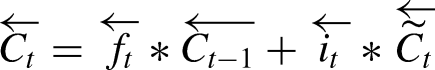
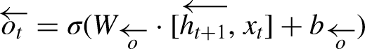
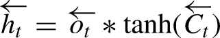
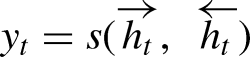
Bi-LSTM networks extend the capabilities of standard LSTMs by processing data in both forward and backward directions, which allows the model to leverage context from both the past and the future for improved prediction accuracy.
In a Bi-LSTM, the forward LSTM processes the sequence from start to end, described by: (Singla et al., 2022b)
Metrics
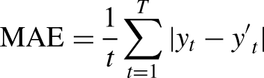
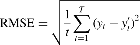
RMSE is widely used for evaluating solar forecasting models because it penalizes large errors, which are highly undesirable in this context. MAE is also used but are scale-dependent and best suited for results with Gaussian distributions (View of Review of Different Error Metrics: A Case of Solar Forecasting, n.d.). MAE measures the average absolute difference between the predicted and actual prices over the entire test dataset.
Mathematically, MAE is calculated as:
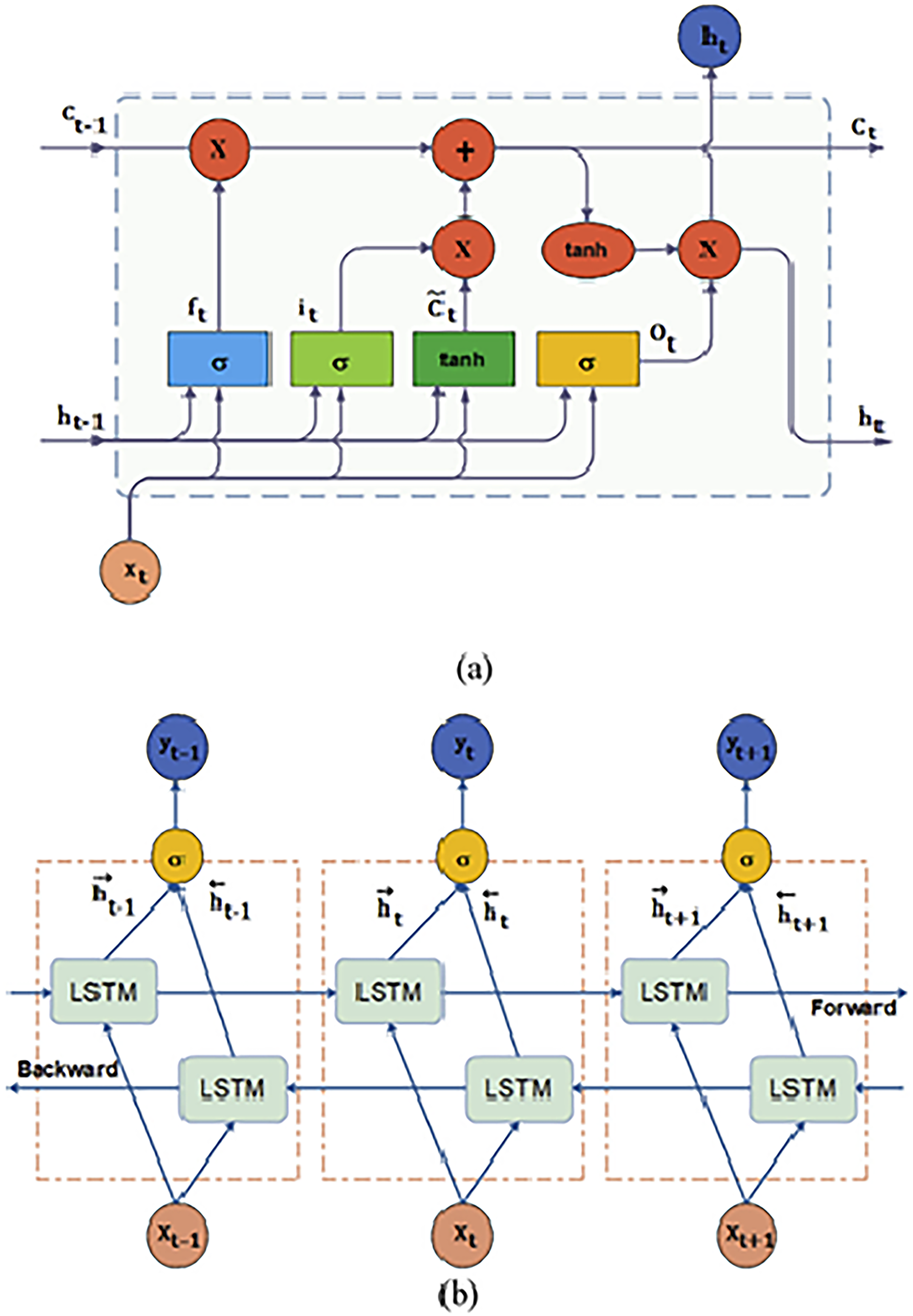
Architecture of (a) LSTM (b) Bi-LSTM (Sharadga et al., 2020).
Results and discussion
Data visualization
In Figure 2, the temporal dynamics of energy consumption are illustrated over the observed period. The y-axis represents energy consumption, and the x-axis represents time, offering a comprehensive depiction of the fluctuations in energy usage throughout the timeline.
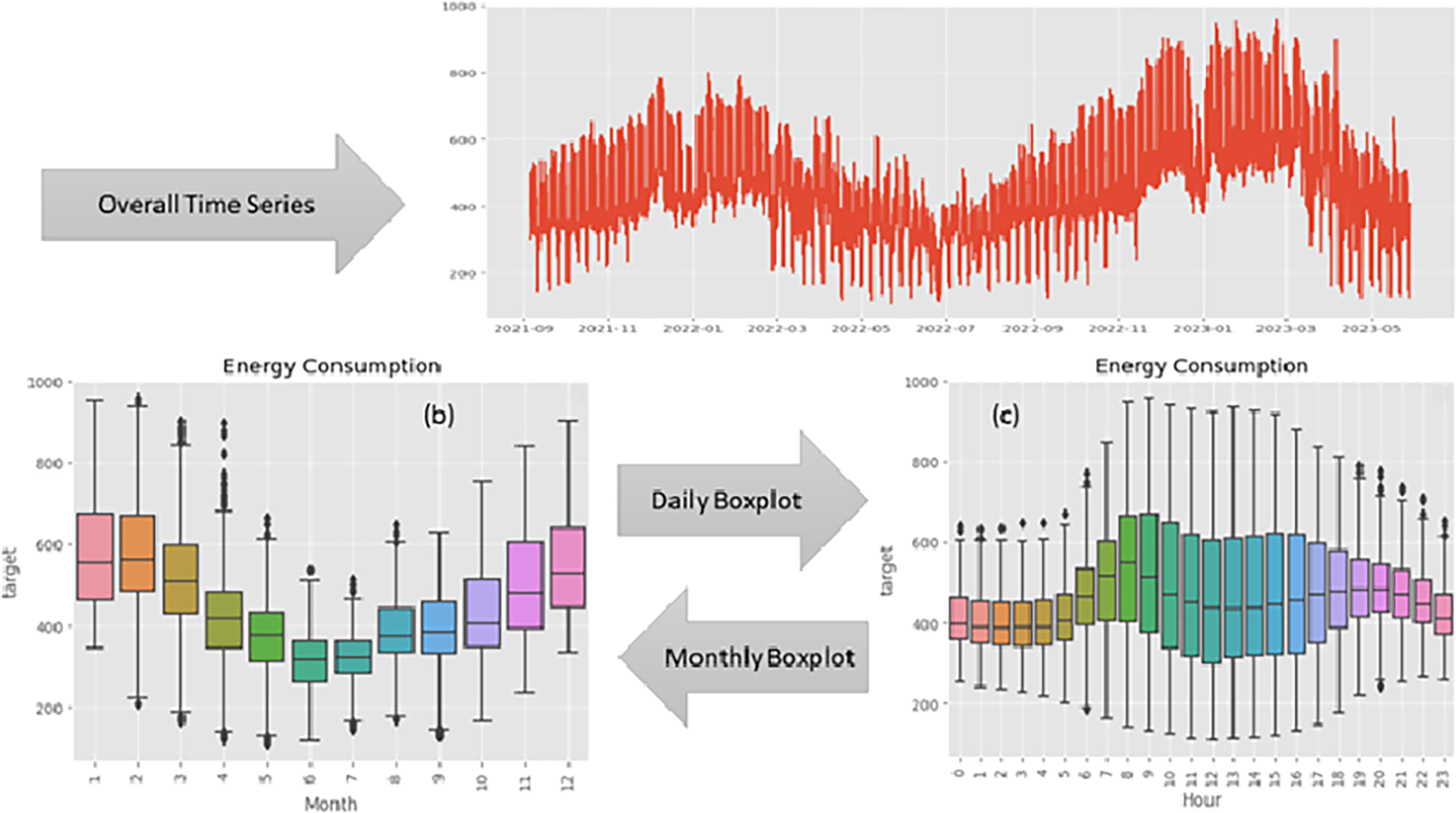
Time series plot of energy consumption. (a) Overall time series. (b) Daily time series boxplot. (c) Monthly time series boxplot.
The plot unveils a distinct pattern, indicating that energy consumption typically hits its lowest points from March to September. In contrast, the months spanning December to February showcase elevated energy consumption levels, reaching a peak during this timeframe. This observable seasonality implies a cyclical trend that may be influenced by diverse external factors, including weather conditions, holidays, or industrial patterns.
Insights drawn from the time series plot play a crucial role in preprocessing time series data. A comprehension of recurring patterns enables well-informed decisions regarding data transformation, feature engineering, and model selection. For instance:
The density plot discernibly exposes a conspicuous concentration of variable values within the interval [1200, 1600]. The heightened density within this range denotes a substantial aggregation of data points, suggesting a critical region within the variable's spectrum.
This asymmetry signifies the existence of data points beyond the primary density concentration, indicating potential outliers or instances of extreme values that diverge from the central tendency (Figure 3).
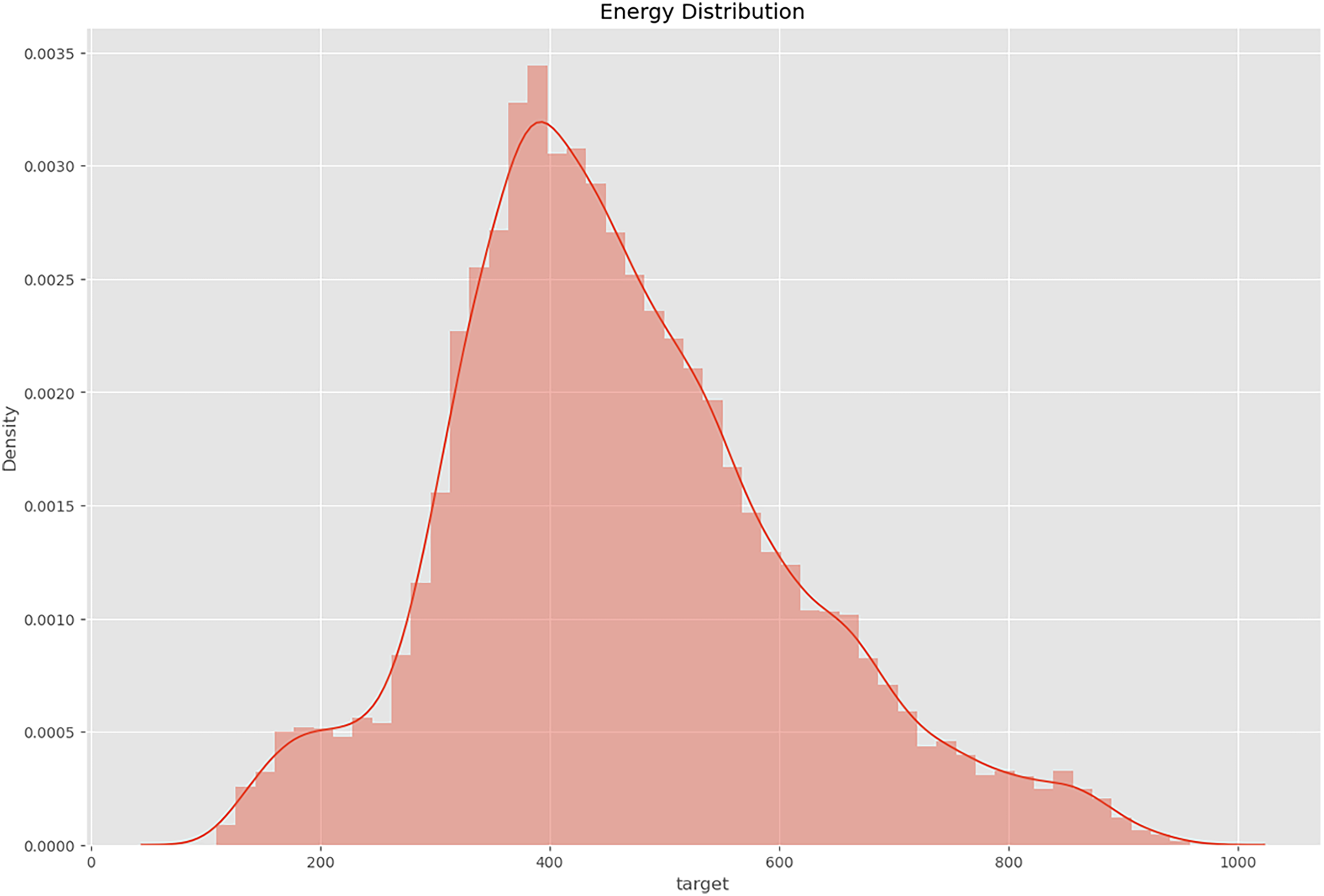
The density plot discernibly exposes a conspicuous concentration of variable values within the interval [1200, 1600].
In summary, the time series plot serves as a valuable tool in the preprocessing stage, enabling data scientists to make informed choices regarding feature engineering, model selection, and other relevant preprocessing steps.
Kaggle dataset
Enefit, a powerhouse in the Baltic energy sector, stands at the forefront of green energy solutions. Their expertise guides customers on a personalized and flexible journey towards sustainable practices, implementing environmentally friendly energy solutions. Despite being armed with internal predictive models and third-party forecasts to tackle energy imbalances, existing methods fall short in accurately predicting the intricate behaviors of prosumers, resulting in substantial imbalance costs.
The use of this Kaggle dataset is justified due to its quality and relevance for studying energy consumption patterns, which is critical for accurate solar irradiance forecasting. This dataset, curated from Kaggle, provides 15,312 observations featuring two key variables: date and time, and energy consumption (Enefit - Predict Energy Behavior of Prosumers | Kaggle, n.d.). This dataset offers a comprehensive perspective on Estonia's energy dynamics, ensuring no duplications. The inclusion of date and time as features is crucial for capturing temporal patterns, while energy consumption serves as the target variable essential for training the forecasting models.
To ensure robust model evaluation, the dataset is split into three parts: 80% for training (12,248), 10% for validation (1532), and 10% for testing (1532). This split allows for thorough training of the model, fine-tuning through validation, and unbiased performance evaluation on the test set.
Acknowledging the constraints of existing forecasting methods, the focus shifts to machine learning (ML), specifically within the domain of time series prediction for energy scenarios. In the face of a progressively intricate energy balance landscape, this study explores the utilization of deep neural networks. Through a thorough examination of complex and imbalanced datasets, considering runtime efficiency and model precision, the research contrasts conventional ML approaches such as ARIMA and SARIMA with advanced RNNs, specifically LSTM and Bi-LSTM.
System requirements
The experiments were conducted on the Kaggle platform, an open-source notebook environment provided by OpenML. This platform offers access to both free and premium GPU (P100) and TPU resources, which are highly beneficial for academic and research purposes. The models were trained using four GPUs, each with 16 GB of RAM. The implementation was carried out in Python, utilizing TensorFlow for the backend and Keras APIs for the frontend of the system.
Prediction analysis
LSTM (long short-term memory)
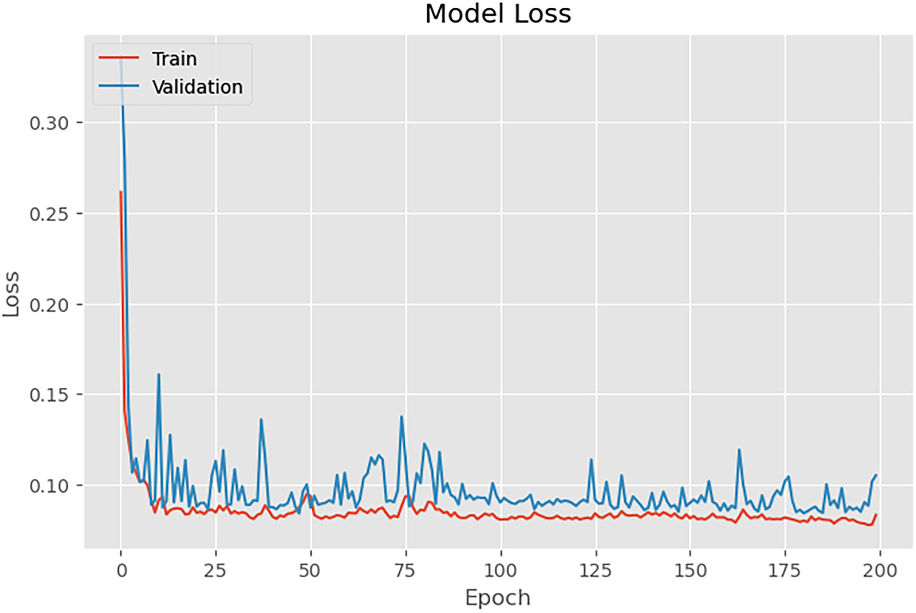
In our quest to decipher the intricate patterns within time series data, we harnessed the power of LSTM networks. The results, as depicted in Figure 4, showcase the convergence of training and validation losses, portraying a model finely tuned and adept at extracting intricate patterns from real-world datasets (Figure 5).
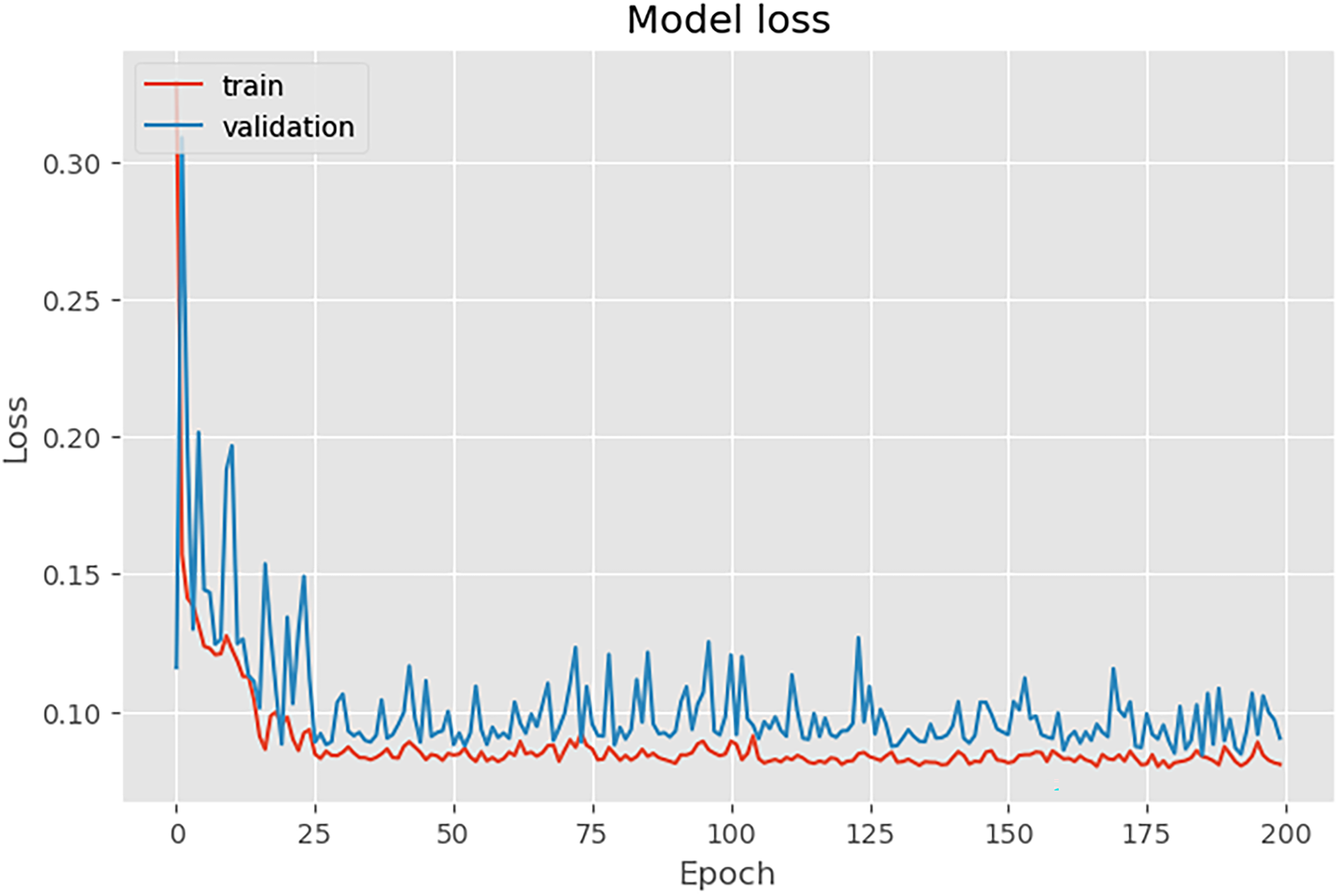
LSTM training and validation losses.
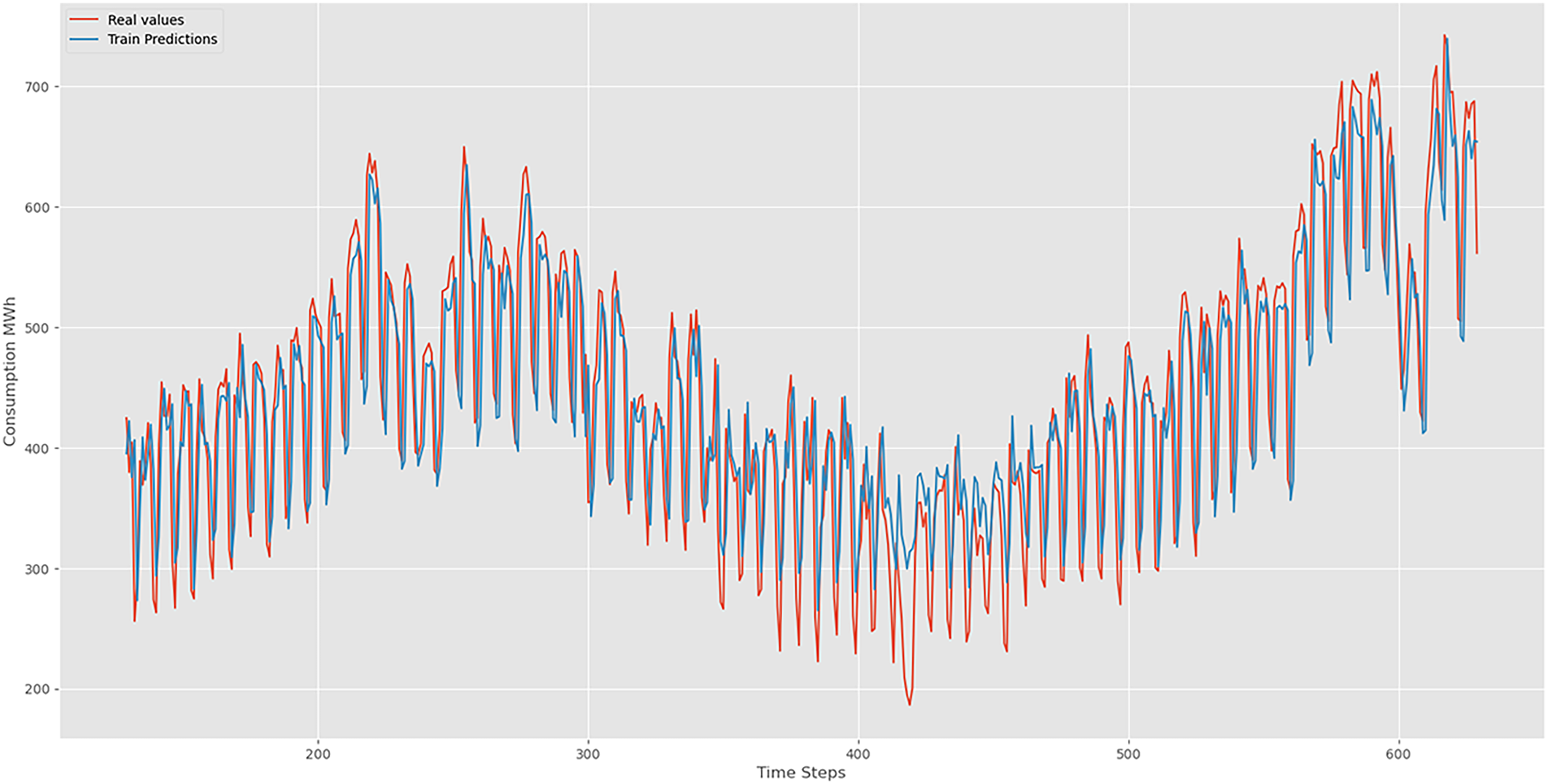
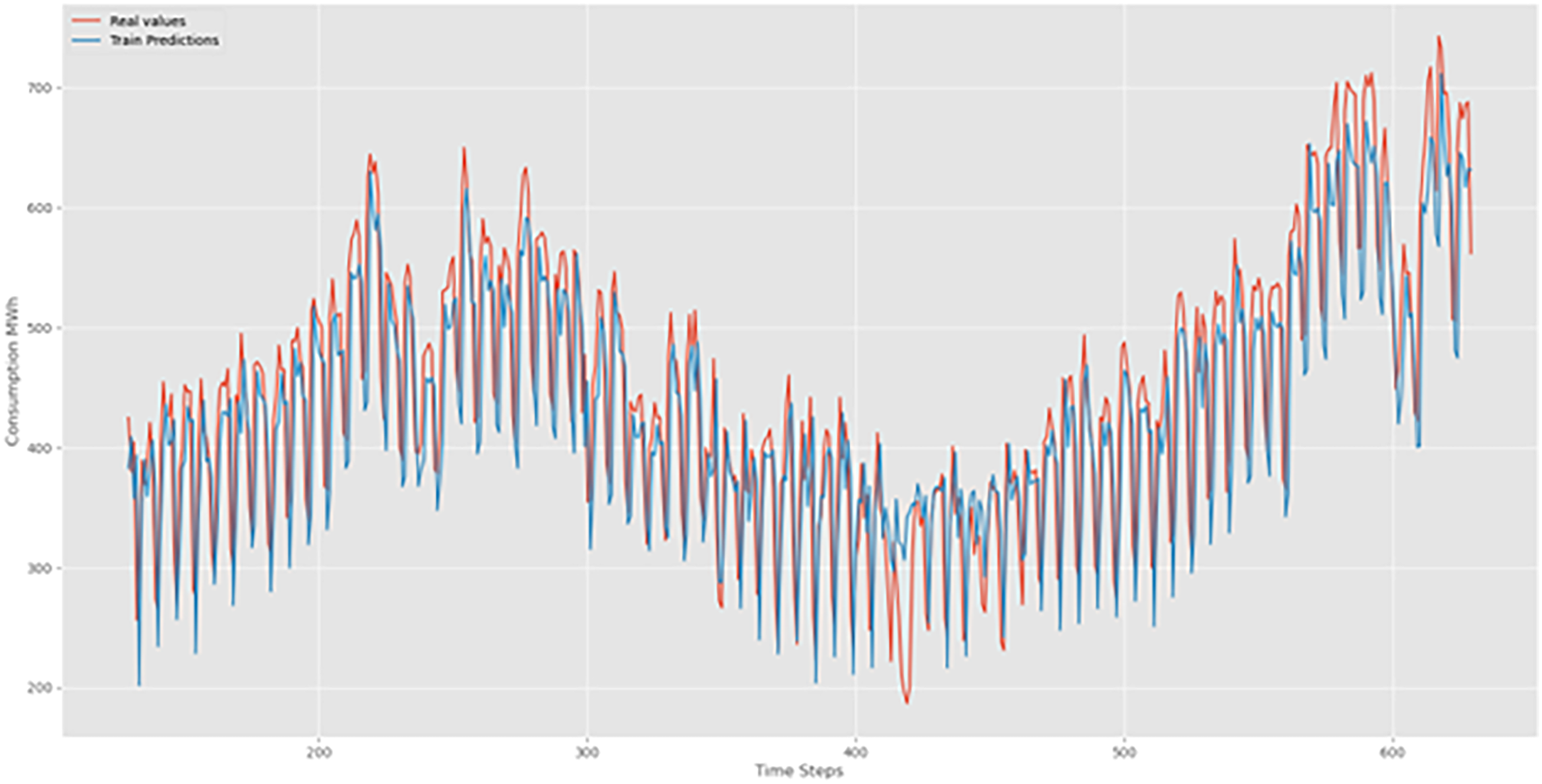
LSTM training prediction.
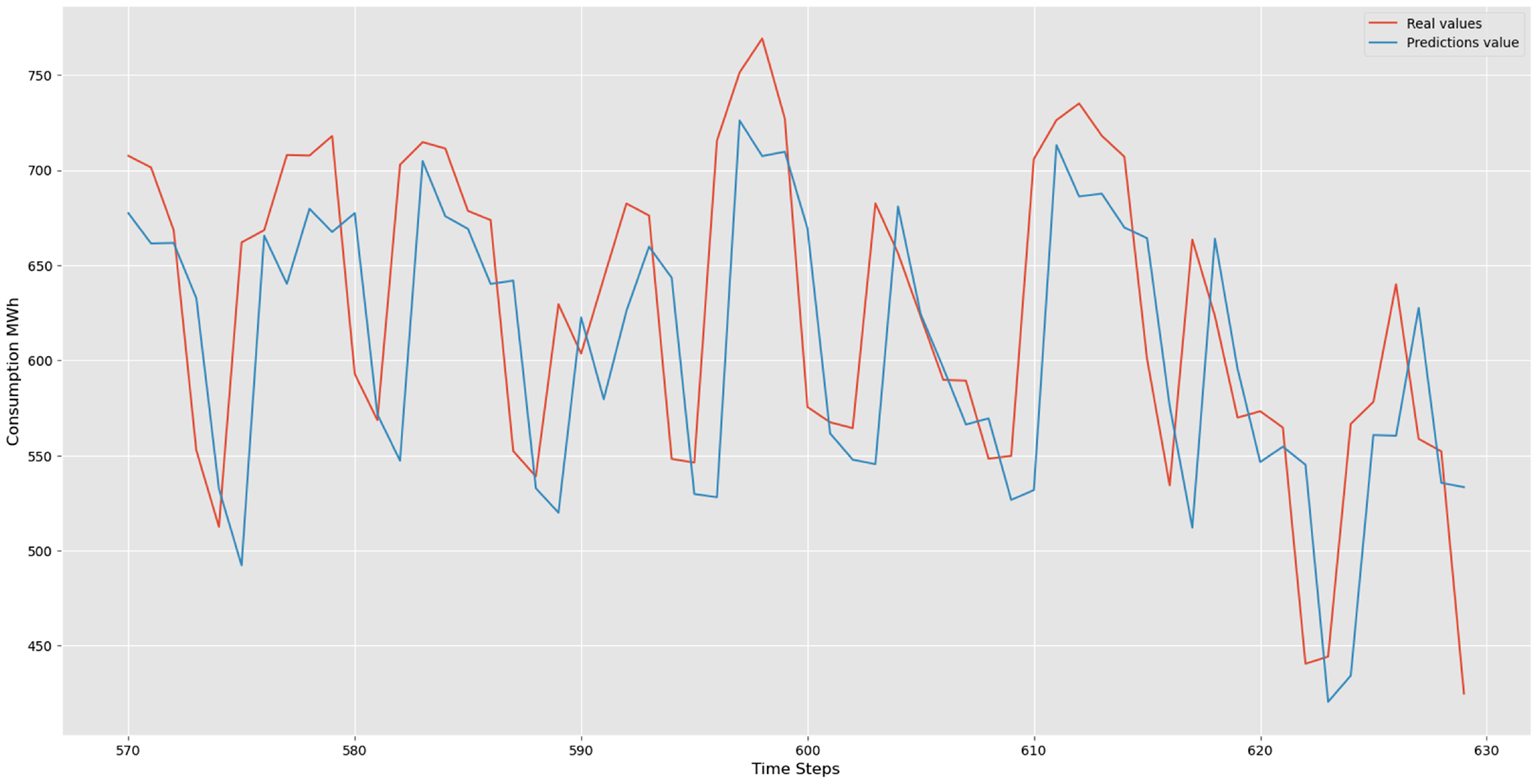
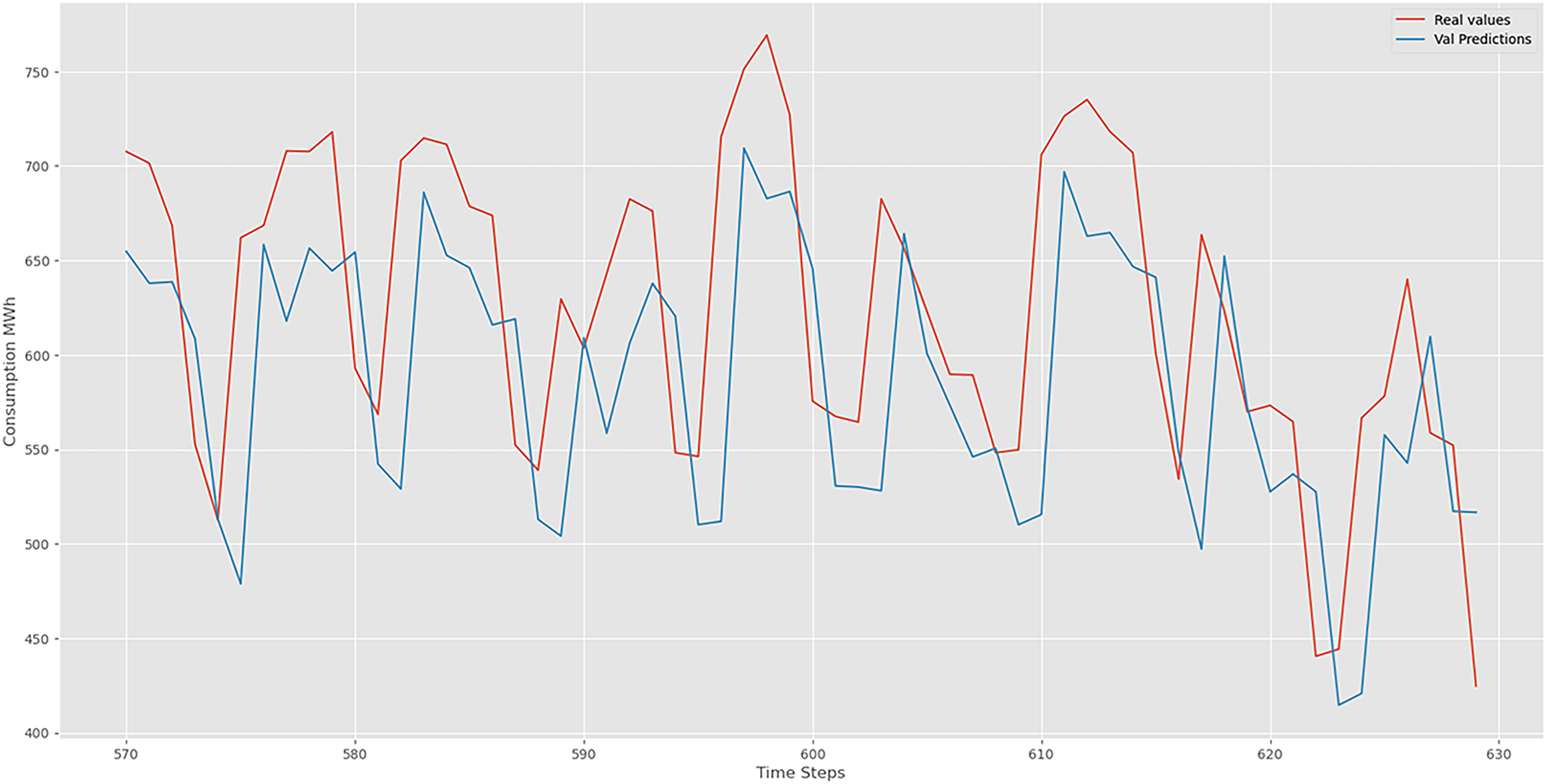
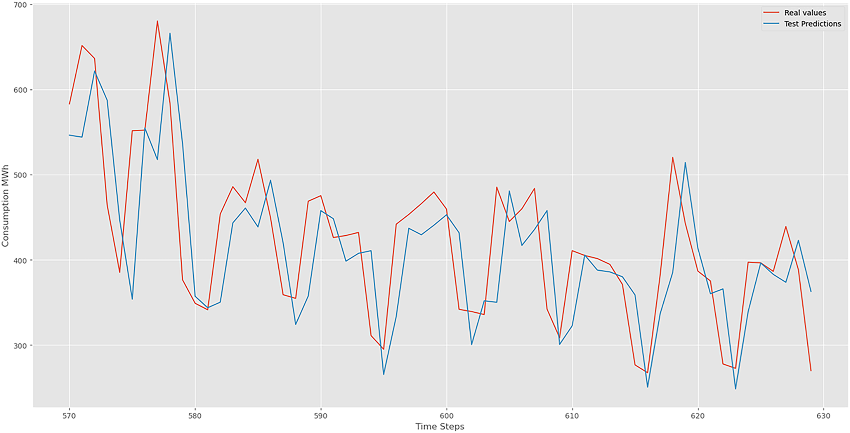
Figures 6 and 7 demonstrate the forecasting capabilities of our LSTM model. Red lines represent actual values, while blue lines depict predicted values. These figures illustrate the LSTM's effectiveness in capturing periodic sequences. The fluctuations between real and predicted values reflect the precision and accuracy inherent in our LSTM model. Our LSTM model excels in accuracy metrics when analyzing complex time series data, revealing temporal patterns with detailed insight.
LSTM validation prediction.
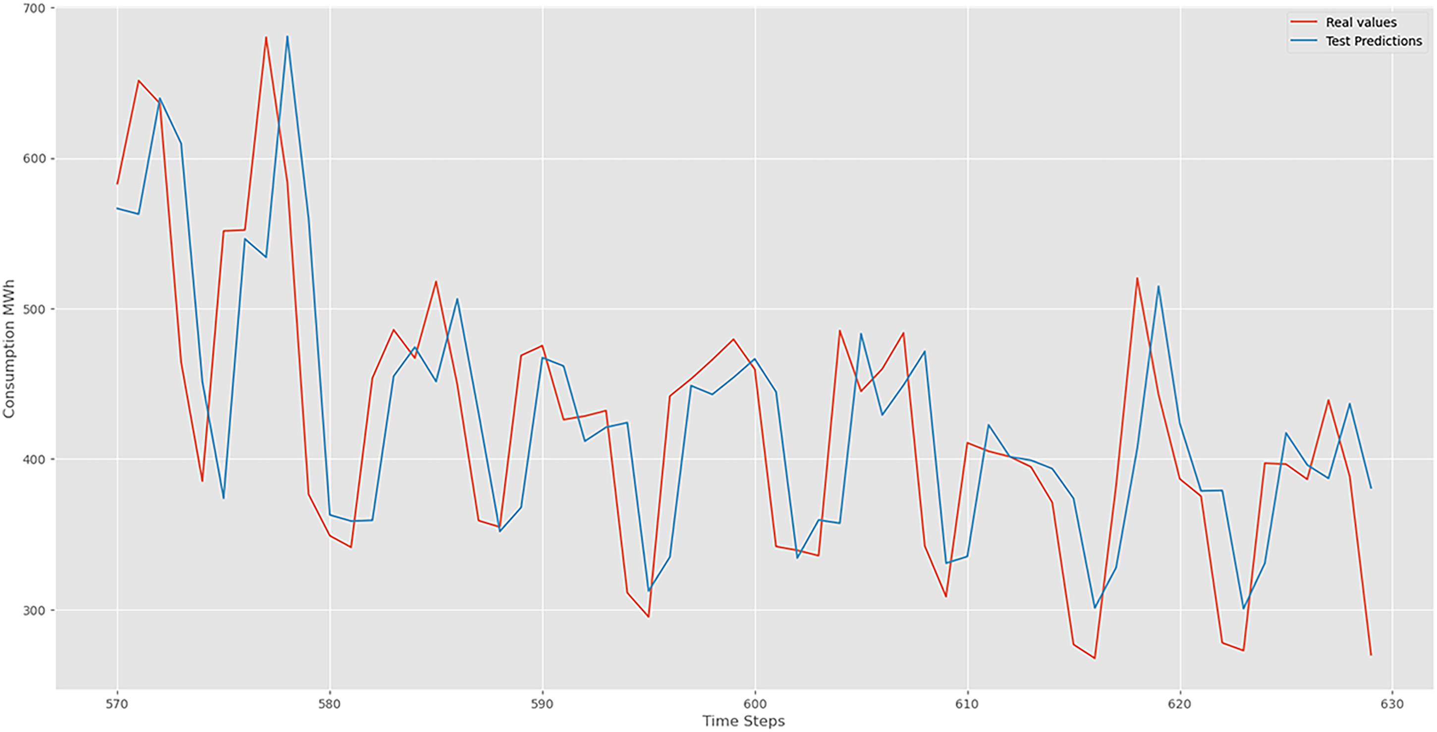
LSTM test prediction.
The results we have obtained from our LSTM model are typically metrics used to evaluate the performance of regression models, particularly in time series forecasting tasks. Here's a brief description of each metric:
Test Data: This metric measures the average absolute difference between the actual and predicted values in our test dataset. In our case, the MAE for the test data is 0.097, indicating an average absolute error of approximately 0.097 units. Train Data: Similarly, for the training dataset, the MAE is 0.079. This suggests an average absolute error of around 0.079 units between the actual and predicted values during the training phase.
Test Data: RMSE is a measure of the average magnitude of the errors between predicted and actual values, giving more weight to larger errors. Our RMSE for the test data is 0.1308, indicating the square root of the average squared differences between the predicted and actual values. Train Data: For the training dataset, the RMSE is 0.112, representing the square root of the average squared errors during the training phase.
These metrics provide insights into the accuracy of our LSTM model. Lower MAE and RMSE values generally indicate better performance, as they suggest smaller errors between predicted and actual values. However, the interpretation of these metrics depends on the specific characteristics and scale of our data.
Bi-LSTM (bidirectional LSTM)
Training loss is compared to the validation loss. The result shows that the two values were low, and no overfitting was detected. The results are shown in Figure 8.
Bi-LSTM training and validation loss.
Examples of consumption predictions of the LSTM model were done using the training dataset (Figure 9), validation dataset (Figure 10), and test datasets (Figure 11).
Bi-LSTM training prediction.
Bi-LSTM validation prediction.
Bi-LSTM test prediction.
The predictive capabilities of our Bi-LSTM model shine through the lens of performance metrics, revealing a nuanced understanding of its effectiveness. In the realm of time series forecasting, the Bi-LSTM model has showcased its prowess on both training and test datasets, delivering impressive results. It is provided the performance metrics as following below:
Train Data: 0.108 Test Data: 0.124 Train Data: 0.076 Test Data: 0.092
The evaluation metrics highlight the Bi-LSTM model's proficiency in handling the dataset's complexities. The lower RMSE and MAE values indicate its accuracy in predicting the target variable, demonstrating a robust fit to both the training and test datasets. These metrics quantify the model's performance, confirming its potential for accurate and reliable predictions in time series analysis.
SARIMA (seasonal autoregressive integrated moving average)
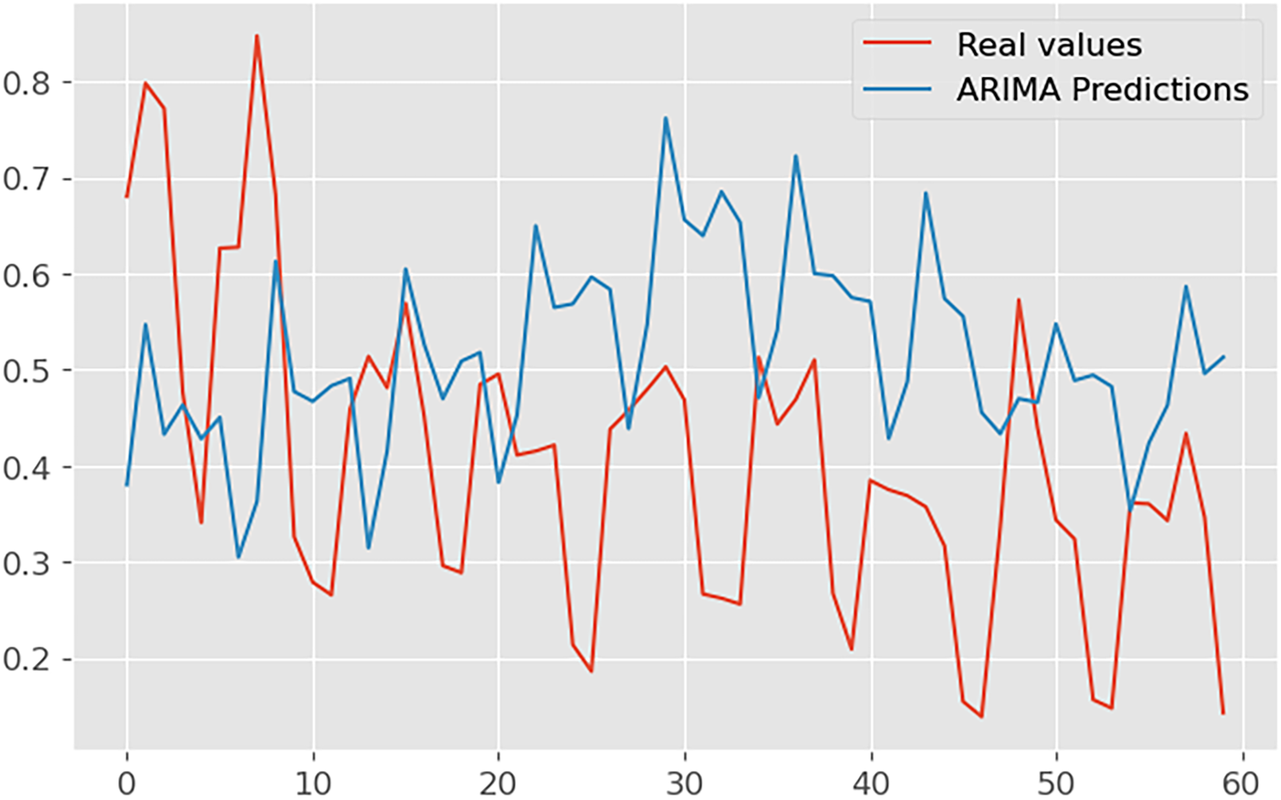
In Figure 12, we present the captivating visual representation of predictions generated by the SARIMA model. This plot gracefully intertwines the actual observed values and the SARIMA-predicted values, painting a vivid picture of the model's forecasting capabilities.
SARIMAX training loss.
The red line gracefully traces the chronological path of the true values, providing a benchmark for the model's accuracy. In harmonious contrast, the blue line intricately weaves through time, representing the SARIMA model's predictions. The seamless alignment of these lines signifies the model's ability to capture the inherent patterns and seasonal fluctuations present in the time series data. Noteworthy is the model's proficiency in handling complex temporal dynamics, as evidenced by its adept prediction of future values. The periodicity and trends ingrained in the dataset are eloquently mirrored by the SARIMA model, establishing its credibility in time series forecasting. The minutely detailed interplay between actual and predicted values showcases the SARIMA model's precision, making it a valuable tool for understanding and anticipating temporal patterns in the dataset.
The SARIMAX results (Figure 13) provide a comprehensive overview of the predictive model's performance on the energy dataset. The model, specified as ARIMA (2, 1, 1) × (1, 1, 1, 12), showcases a detailed breakdown of coefficients, standard errors, statistical significance, and various diagnostic metrics. The SARIMAX model provides valuable insights into the temporal dynamics of the energy dataset. However, the diagnostic metrics highlight areas for improvement, such as addressing potential seasonality and autocorrelation in the residuals to enhance the model's forecasting accuracy.
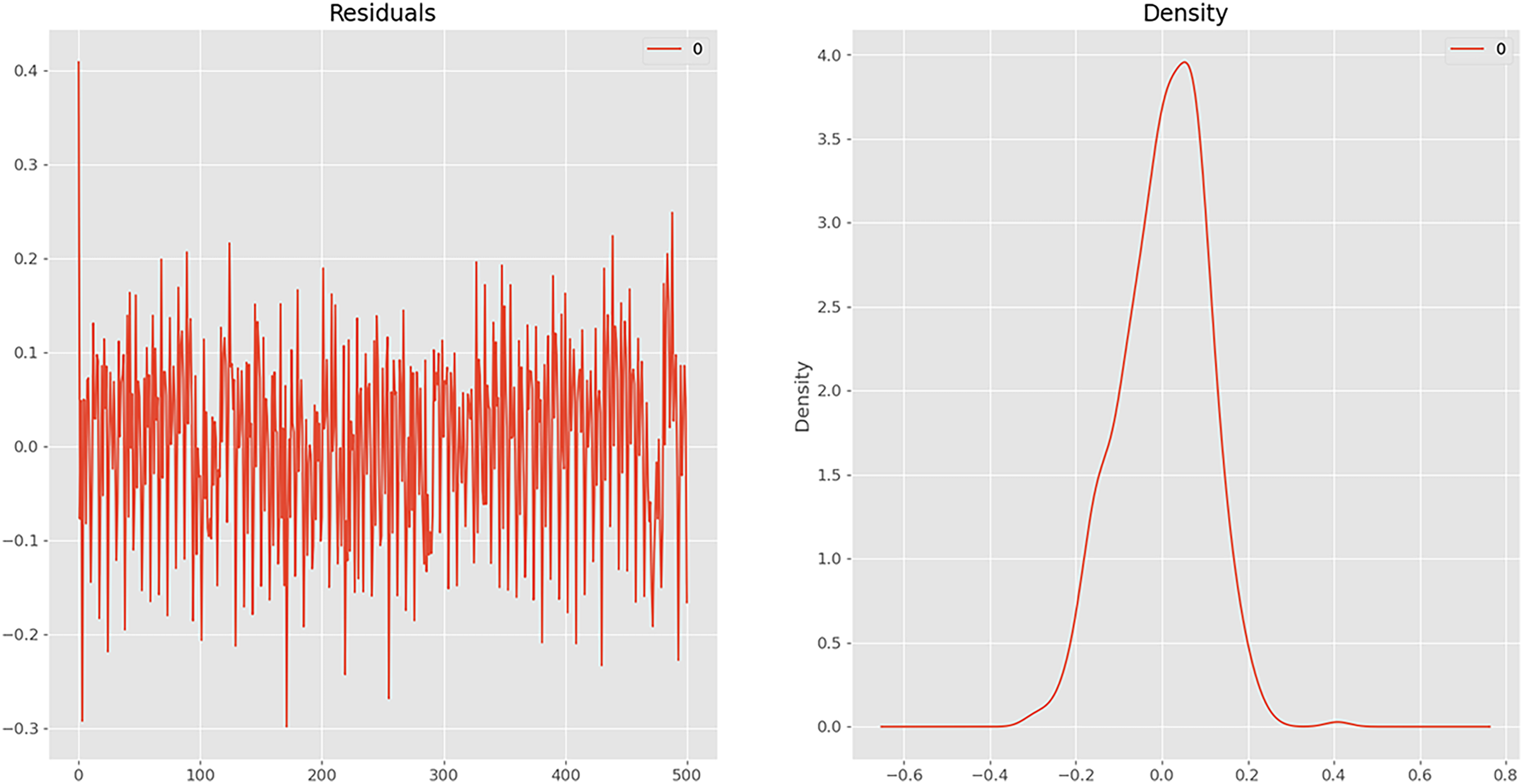
SARIMAX prediction: (a) residuals and (b) density.
Test Data: 0.251 Test Data: 0.203
The performance metrics of four models—LSTM, Bi-LSTM, ARIMA, and SARIMAX—are compared based on MAE and RMSE for both training and testing datasets, as presented in Table 1.
Comparison metrics of models performance.
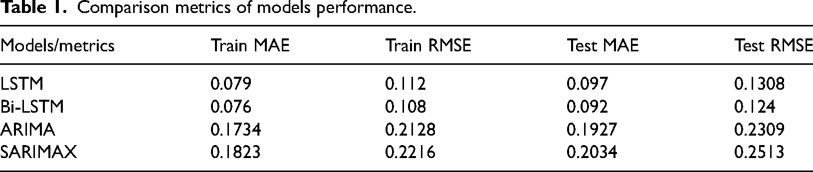
The Bi-LSTM model demonstrates slightly better performance than the LSTM model, with lower Train MAE (0.076 vs. 0.079) and Train RMSE (0.108 vs. 0.112). On the test set, Bi-LSTM also outperforms LSTM, achieving lower Test MAE (0.092 vs. 0.097) and Test RMSE (0.124 vs. 0.1308). This indicates Bi-LSTM's enhanced ability to capture complex patterns and dependencies in the data.
Comparing LSTM and Bi-LSTM with ARIMA and SARIMAX, it is evident that LSTM and Bi-LSTM significantly outperform the traditional statistical models. For example, the Train MAE for LSTM (0.079) and Bi-LSTM (0.076) are much lower than ARIMA (0.1734) and SARIMAX (0.1823). Similarly, on the test data, both LSTM and Bi-LSTM achieve much lower Test MAE and Test RMSE compared to ARIMA and SARIMAX. Bi-LSTM has the lowest Test RMSE (0.124), followed by LSTM (0.1308), while ARIMA and SARIMAX exhibit higher errors (Test RMSE: 0.2309 and 0.2513, respectively).
Overall, Bi-LSTM emerges as the best-performing model among the four, followed closely by LSTM. Both deep learning models outperform the traditional ARIMA and SARIMAX models, which exhibit higher error rates in both training and testing phases. This analysis underscores the efficacy of advanced NN architectures, particularly Bi-LSTM, in delivering more accurate energy consumption forecasts compared to traditional statistical methods. The results suggest that for applications requiring high precision in time series forecasting, leveraging deep learning approaches like LSTM and Bi-LSTM is advantageous.
On the other hand, to compare externally our work with the recent research worked on the same dataset, Chandran and Narayanan (2024) were the only researchers to have worked on this dataset, using Linear Regression, MLP, TabNet, XGBoost, LightGBM, and VotingRegressor-based ensemble models. Their work resulted in a MAE of 74.56, with the VotingRegressor ensemble being the best-performing model with an MAE of 70.16. Since this Kaggle dataset was launched only a few months ago, no other research has been published on it, and no standardized processing methods have been established. As a result, we are unable to provide a proper comparison of our results with external published papers.
Limitations
Despite the promising results, this study acknowledges several limitations that warrant future research. First, the computational complexity of LSTM and Bi-LSTM models requires significant resources and training time, and optimization techniques to reduce this overhead were not explored. Second, the models were tested on specific datasets, and their generalizability to other types of time series data remains unverified, necessitating broader dataset evaluations. Third, the study focused on univariate forecasting without incorporating additional contextual features, such as weather conditions or economic indicators, which could enhance accuracy. Lastly, deep learning models, despite their accuracy, often lack interpretability compared to traditional statistical models, highlighting the need for improved transparency and understanding in future studies.
Future study
Future research should aim to address the limitations identified in this study to improve the applicability and performance of time series forecasting models. Optimization techniques need to be explored to reduce the computational complexity and training time of LSTM and Bi-LSTM models, making them more feasible for real-time applications. Additionally, evaluating these models on a wider range of datasets will help determine their generalizability and robustness across different domains. Incorporating multivariate forecasting by including contextual features, such as weather conditions and economic indicators, could enhance predictive accuracy. Lastly, developing methods to improve the interpretability of deep learning models will be essential for making these advanced techniques more accessible and transparent to stakeholders and decision-makers.
Conclusion
Figures 6, 7, 10, and 11 shows some delay between actual and predicted values in energy consumption. This discrepancy is attributed to the dynamic nature of energy consumption patterns among consumers, which do not consistently adhere to predefined patterns due to various influencing factors. In our subsequent study, we will explore the influence of environmental parameters on energy consumption prediction. Environmental factors such as weather conditions, seasonal variations, and other external influences can significantly impact energy usage patterns.
Predicting energy consumption has become increasingly vital in our daily lives, given its significant economic implications. Various methods have been devised for energy consumption forecasting. However, conventional techniques often fall short as they fail to capture the periodic patterns inherent in energy consumption data. This paper introduces a comprehensive approach to time series prediction with periodicity, leveraging LSTM and Bi-LSTM as RNNs, in conjunction with ARIMA and SARIMA as ML models. The comparison is applied to these models based on the datetime feature under one-step-ahead forecasting. The important findings of this study are brought below to get a look at easily:
The proposed model presents a promising approach for forecasting the time-series energy generated by both consumers and prosumers. It offers an alternative solution for delivering reliable predictions. Utilizing the time variable enables precise capture of periodicity. Incorporating this variable into the LSTM model enhances accuracy in predicting energy consumption. Furthermore, the Bi-LSTM method demonstrates superior prediction performance compared to LSTM, ARIMA, and SARIMA models.
The RMSE of Bi-LSTM is 5.35% lower than LSTM, 46.08% lower than ARIMA and 50.6% lower than SARIMA in the forecasting of long-term time series. The MAE of Bi-LSTM is 5.15% lower than LSTM, 52.08% lower than ARIMA and 54.18% lower than SARIMA in the forecasting of long-term time series. Optimal parameter configuration plays a pivotal role in determining the performance of the LSTM model. Careful consideration should be given to selecting the training epoch to prevent insufficient training and overfitting issues. Introducing additional hidden layers can enhance the accuracy of both Bi-LSTM and LSTM models to some degree, albeit at the expense of increased computational time. This research showcases the promising potential of the proposed approach in forecasting energy consumption. Future investigations will concentrate on developing a hybrid model that combines LSTM with other forecasting techniques for enhanced accuracy in energy consumption predictions.
Footnotes
Declaration of conflicting interests
The authors declared no potential conflicts of interest with respect to the research, authorship, and/or publication of this article.
Funding
The authors received no financial support for the research, authorship, and/or publication of this article.