Sage Journals: Discover world-class research

Abstract

This study presents a novel approach that employs a mixture of the tunable-Q wavelet transform (TQWT) and enhanced AdaBoost to address the issue of high impedance fault (HIF) recognition in power distribution networks. Traditional overcurrent protection relays frequently have lower fault current levels than normal current, making it exceedingly difficult to detect this HIF problem with the necessity to use a quick and effective approach to find HIF problems. Since the TQWT performs better with signals that exhibit oscillatory behavior, it has been utilized to extract special features for the training of the improved AdaBoost model. The procedure is accelerated by calculating the Kourtosis (K) value for each level and selecting the ideal level of decomposition to minimize computing work. Faulted zones are categorized using an enhanced AdaBoost approach. Under normal, noisy, and unbalanced conditions, the recommended approach is applied to an imbalanced 123-bus test system and an IEEE 33-bus test system. The efficiency of the recommended method is also being assessed for imbalanced distribution networks incorporating dispersed generation into real-time platforms. This procedure is quick compared to previous methods since it uses an upgraded AdaBoost classifier and optimal decomposition level.

Keywords

AdaBoost classifier fault diagnosis graph theory optimization technique signal processing

Introduction

In recent days, maintaining the desired quality of voltage and current waveforms in power distribution systems (PDSs) has become a tedious task. With the introduction of a deregulated form of power system operations with the involvement of the smart grid concepts, it has become a vital task to identify the sources of harmonic pollution. When a fault happens in the PDS, the reference voltage and current levels deviate, causing abnormal current levels to flow through the distribution system. This can damage PDSs equipment and cause cascading failures in power system operation. To minimize this blackout, the stable operation of PDSs requires rapid identification of faults (; Ibrahim et al., 2023; Mahmoud et al., 2022; Oliveira and Bollen, 2023).

Electrical faults are broadly separated into two categories: open circuit and short circuit (SC) faults (symmetrical and unsymmetrical faults). In the PDSs, 70–80% of the faults that occur are the L-G faults, 15–20% are the L-L faults, and 10% are the L-L-G faults. When a single conductor connects to the ground or a neutral conductor, then there will be an L-G problem. High impedance fault (HIF) happens when a wire brand contact with ground either sand or any ground object that resists the passage of fault current (FC) to a level lower than that can be detected by traditional overcurrent relays (OR). The HIF is difficult for traditional OR to detect (Mahmoud et al., 2023; Veerasamy et al., 2021).

Implementing a long short-term memory (LSTM) method based on recurrent neural networks (NNs) for the identification of HIF under the effect of PV installations was performed by (Veerasamy et al., 2021). Using convolutional NNs, a deep reinforcement learning system for HIF identification was created (Elmetwaly et al., 2023; Teimourzadeh and Member, 2021). Suggest a technique that uses the impedance angle method to identify and categorize HIF from SC failures and other switching and load transients (Dubey and Jena, 2020). Wishing-for a HIF detection method based on the feeder terminal units to locate HIF in single-phase PDSs by calculating the transient zero sequence admittance was done by (Li et al., 2022). Formulating a computational approach termed relative skewness for the detection of the asymmetry introduced by the HIF in the feeders of the PDSs was done in Ozansoy (2020). The wavelet transforms (WT) for extracting characteristics from HIF current signals and the NNs for HIF detection were employed to create a unique HIF detector known as the improved feeder terminal unit. A HIF detection method based on a feeder terminal unit was represented by (Gu et al., 2021). Utilizing a NN to locate HIF in a medium voltage unbalanced PDS was done in (Ledesma et al., 2021). Analyzing the performance of various signal-processing techniques in detecting HIF was presented in (Hamatwi et al., 2023). Proposing a feature selection approach, for HIF diagnosis and identification, where a methodical feature extraction model has been implemented. The HIF characteristics are retrieved based on the time duration and the site of the fault occurrences (Sheng et al., 2024). A variational prototyping encoder in the PDS for the HIF discovery way based on zero sequence current characteristics and a decision tree classifier was proposed by (Xiao et al., 2022). A state space equation-based HIF finding was proposed for the active PDS by (Wang and Cui, 2022). An HIF detection approach in the microgrid with the usage of discrete WT (DWT) and support vector machine (SVM) was developed by (Varghese P et al., 2023). A combined approach built on wavelet-fuzzy to detect and classify HIF in PDSs was provided in Silva et al. (2020). A novel feature harvest technique for identifying HIF faults has been devised, applying the tunable-Q wavelet transform (TQWT), wherein the filters are designed to obtain the fundamental frequency component (FFC) from the full voltage/current signal. This is achieved by varying the redundancy (r) and Q-factor (QF) of the wavelet, primarily by searching for harmonics near the FFC (Tu et al., 2017).

The TQWT is versatile when it comes to identifying disturbances that have taken place in the signals and is also capable of simply extracting the FFC of the signal. Because of this, researchers used defect identification algorithms to a far greater extent. A technique for diagnosing power quality disturbances (PQD) utilizing TQWT and SVM classifier-based techniques was suggested by (Thirumala et al., 2018). There is a proposal in that paper for TQWT-based bearing defect diagnostics under time-varying fields (Shi et al., 2019). TQWT has also been used to identify defects in railway axle bearings since it was deployed (Ding et al., 2019). A technique to detect a fault in a momentary gearbox was proposed by Zhang et al. (2022) and Ibrahim et al. (2023). PQDs are diagnosed using knowledge-based NNs and TQWT-based methods, both of which are addressed in this article (Izadi and Mohsenian-Rad, 2022). The modified AdaBoost approach is used to identify fault zones in this paper. When compared to other algorithms, this one has benefits in terms of its level of accuracy.

The improved AdaBoost technique (AT) is a very effective feature extraction technique. However, if challenging samples are present in the training samples and the sum of iterations increases, this with no trouble results in the degeneration phenomenon and reduces the classifier’s capacity for generalization. This paper proposes the LWE-AT, which can edge weight extension. The investigational findings show that the LWE-AT can effectively control the repetition of the deterioration singularity in light of look finding under complex background degeneration problems (Shaowen and Yong, 2015). The speed of this algorithm is high and simple. The total amount of repetitions is the only parameter that needs to be changed in this case. This methodology doesn't require any prior understanding of weak knowledge and can be combined with any approach to find a weak premise (Tu et al., 2017). Training and generalization errors of AT were analyzed by (CAO et al., 2013; Mahmoud et al., 2022) which proves its accuracy in all aspects. In (Zhang et al., 2019) the outcomes demonstrate that the AT can classify data sets of different sizes with improved accuracy. The novel technique suggested in this paper is superior to the conventional SVM since it is somewhat fast in terms of calculation speed.

Major contributions

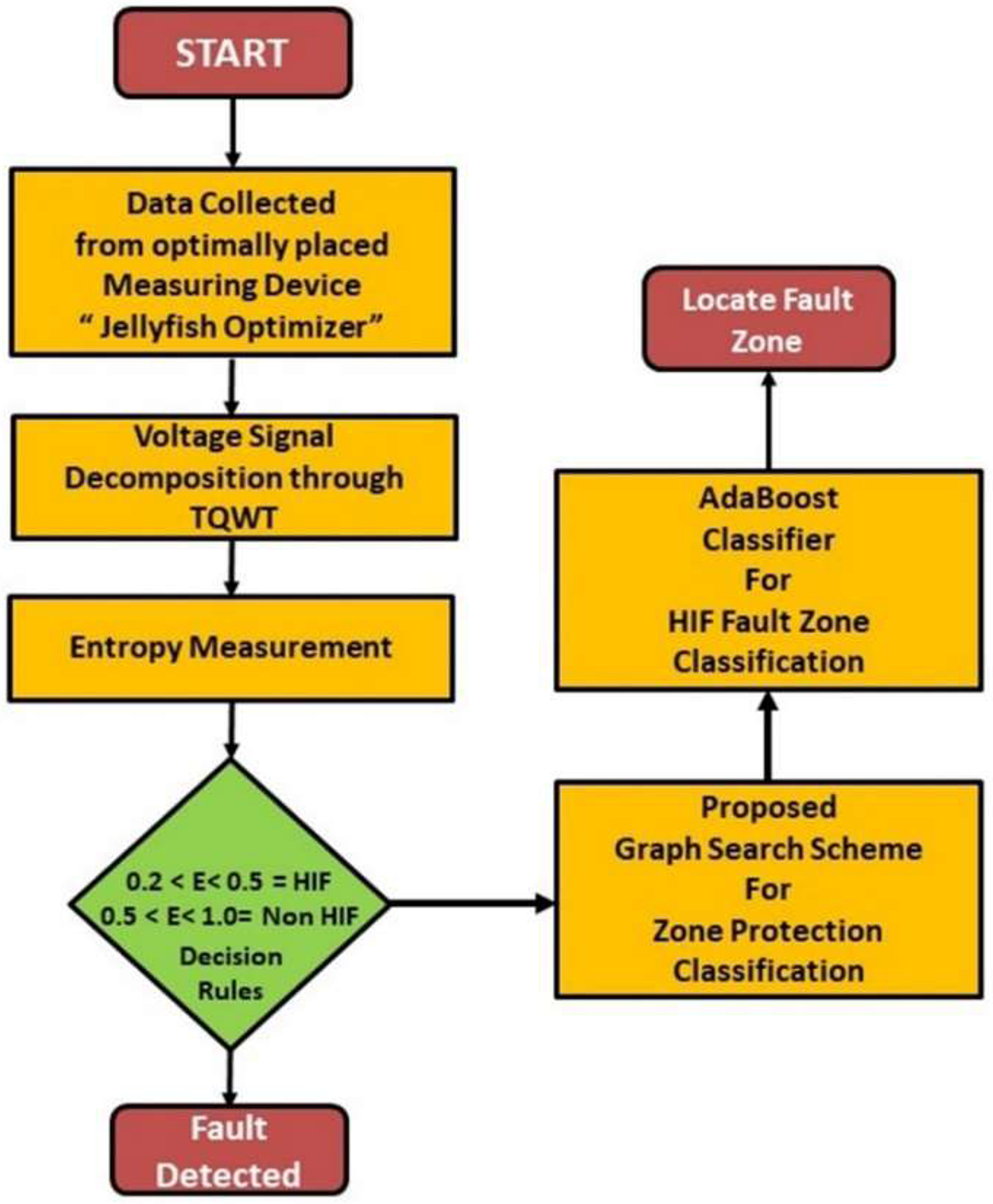
The proposed TQWT-based protection approach delivers a fast, reliable, and effective scheme for detecting faults and fault zones using optimally placed meters. The performance of this method is insensitive to the presence of distributed energy (DG) and noise, as well as harmonics. Choosing the right level of decomposition makes this scheme very fast. Tests achieved with the implementation of the proposed technique on both the platforms of MATLAB/Simulink and Real Time Digital Simulator (RTDS) show that the scheme works in real time. The HIF-WT is required to extract the coefficients. A major addition to the existing body of knowledge in this work is the development of new protection schemes for PDSs based on signal-processing and machine learning classifiers. Based on this scheme, numerical relays can be designed to identify, classify, and locate fault zones in PDSs. The authors have used a completely new approach based on graph theory and the jellyfish search optimizer to locate surveillance devices to identify protection zones within the PDSs. Classify these protected zones using an improved AdaBoost classifier. To analyze signal behavior, TQWT has been used to decompose good and impaired signals based on signal analysis and normalized entropy. The HIF and non-HIF can be distinguished from normalized entropy values. The proposed method provides an accurate algorithm that can identify and classify defects in both normal and noisy, imbalanced circumstances. The suggested approach is also an algorithm that can be generalized and works well even if the structure of the network changes. Real-time experiments also demonstrate the TQWT usefulness. The novel contributions to the proposed method include:

TQWT has been used for the feature extraction from signals as its execution involves an optimal restoration overestimated filter bank with real-valued sampling factors and is built on a dilation factor.

Selection of optimized decomposition level by calculating Kourtosis (K) value to reduce computational burden and make the method fast.

Fault zone detection based on graph theory concept

Selection of optimized measuring points based on Jellyfish search optimizer to make it cost-effective

Normalized entropy calculation which is castoff as a standard for different PDSs.

DG and diverse power electronic devices are considered during fault classification.

Distinguishing between non-HIF and HIF has been done by calculating normalized entropy.

An unbalanced large network has been considered here for verification of the TQWT.

Real-time verification of the TQWT is also shown in the paper.

The problematization of the issue

Simulation of the HIF

To model the HIF, various methods can be used, including analytical, numerical, and experimental approaches. One commonly used method is the analytical approach, which involves solving a set of differential equations that describe the actions of the system during a fault. The analytical model of an HIF involves modeling the fault as a nonlinear element, such as a variable resistor, and incorporating it into the system equations. This allows the calculation of the FC and voltage, which can be used to locate the fault and assess its impact on the system. Another approach is the numerical method, which involves simulating the behavior of the system using computer software. This method can provide more accurate results than the analytical method, but it requires a more detailed model of the system and is more computationally intensive (Jalil et al., 2021; Metwally Mahmoud, 2023). Experimental methods involve creating physical models of the system and observing its behavior during a fault. This can offer insightful information on how the system behaves and can be used to validate analytical and numerical models. Overall, modeling a HIF requires a thorough understanding of the system and its behavior during a fault, and can be done using a variety of analytical, numerical, and experimental methods (Gautam and Brahma, 2013). This model referred to (Gautam and Brahma, 2013) has taken into consideration the HIF model in the study that has been suggested. The simpler HIF model that has been developed as a basic graphic that may be depicted in Figure 1 (Gautam and Brahma, 2013).

Figure 1.

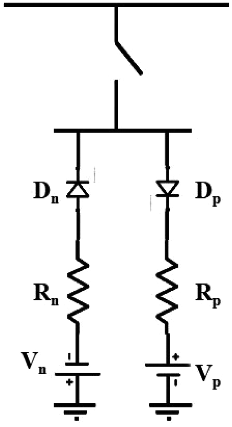
The simplified depiction of the Emmanuel Model of HIF.

Method for the decomposition of signals based on the TQWT

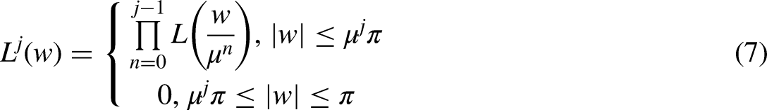
The TQWT is a time-frequency (TF) analysis technique that has been broadly used in signal-processing applications, such as speech and image processing, biomedical signal investigation, and communication systems. The TQWT is a modified version of the DWT, which provides better TF localization and improved frequency resolution (Jalil et al., 2021). The main difference between the DWT and TQWT is that the latter uses a variable QF, which regulates the bandwidth (BW) of the WT function. It is a measure of the QF of a resonant system and is inversely proportional to the BW. A high QF results in a narrow BW and high-frequency resolution, while a low QF results in a broad BW and low-frequency resolution. The length of the signal is what determines the number of stages that are used in this WT. In the TQWT, the QF is adjusted for each frequency band, which allows for better control of the trade-off flanked by time and frequency tenacity. This is achieved by modifying the filter coefficients of the WT using a tunable parameter that controls the QF. The TQWT has several advantages over the DWT. Firstly, it provides better TF localization and improved frequency resolution. This is because the QF can be adjusted to match the signal characteristics, which allows for better separation of frequency components. Secondly, it is more flexible and adaptable to different applications. The tunable parameter allows for optimization of the WT for different signal types and applications. A subband signal with sampling rates is produced as a consequence of filters with a combination of Low pass (LP) and High pass (HP) characteristics used in the first level of decomposition. For $μ f_{s}$ , and $δ f_{s},$ f_s is the frequency at which the input sign v(n) is sampled. The necessary and sufficient conditions for scaling factors are $μ$ and $δ$ (Joga et al., 2021b; Yuan et al., 2024).

0 < μ < 1, 0 \partial \leq 1, μ + \partial 1.

(1)

It is possible to achieve flawless reform by representing the high pass filter (PF) H(w) and the low PF L(w)as:

H (w) = {\begin{matrix} 0, | w | \leq (1 - \partial) π \\ θ (\frac{μ π - w}{μ + \partial - 1}), (1 - \partial) π < | w | < μ π \\ 1, μ π \leq | w | \leq π \end{matrix}

(2)

L (w) = {\begin{matrix} 1, | w | \leq (1 - \partial) π \\ θ (\frac{w + (\partial - 1) π}{μ + \partial - 1}), (1 - \partial) π < | w | < μ π \\ 0, μ π \leq | w | \leq π \end{matrix}

(3)

where ɵ(w)is the frequency response of the fundamental wavelet “db” with:

θ (w) = \frac{(1 + \cos w) \sqrt{2 - \cos w}}{2}, | w | \leq π

(4)

To make a low PF and a high PF as perfect reform, the next conditions ought to be satisfying.

| H (w) |^{2} + | L (w) |^{2} = 1

(5)

Both the low PF and the high PF are broken down into their component parts, and the results are examined and represented as:

H^{j} (w) = {\begin{matrix} H (\frac{w}{μ^{j - 1}}) \prod_{n = 0}^{j = 2} L (\frac{w}{μ^{n}}), w_{1} \leq | w | \leq w_{2} \\ 0, w \notin [- π, π] \end{matrix}

(6)

L^{j} (w) = {\begin{matrix} \prod_{n = 0}^{j - 1} L (\frac{w}{μ^{n}}), | w | \leq μ^{j} π \\ 0, μ^{j} π \leq | w | \leq π \end{matrix}

(7)

where

w_{1} = (1 - \partial) μ^{j - 1} π, w_{2} = μ^{j - 1} π

, the TQWT decomposition depends mostly on scaling settings, QF, and filters. The ratio of the filter's center frequency w_central to its BW gives the QF its definition.

Q = \frac{w_{central}}{BW}

(8)

The definition of BW may be constructed according to Equation (7) and it is represented as

BW = \frac{w_{2} - w_{1}}{2} = \frac{\partial μ^{j - 1} π}{2}

(9)

It is possible to arrive at the formula for the central frequency w_central by averaging the weights w₁ and w₂, and the resulting value may be expressed as

w_{central} = \frac{w_{1} + w_{2}}{2} = \frac{(2 - \partial) μ^{j - 1} π}{2}

(10)

From Equations (8) and (9), the Q.f can be represented as:

Q . f = \frac{w_{central}}{Bandwidth} = \frac{2 - \partial}{\partial}

(11)

From Equation (11), It has been discovered that the Q.f is solely determined by the high pass scaling factor ə. It is stated as the rate of dismissal factor r as in Equation (12):

r = \frac{\partial}{1 - μ}

(12)

Several factors, including the

\partial

μ

, and Q.f, and the idleness factor, are all connected to one another in the manner that is detailed below:

\partial = \frac{2}{(Q . f + 1)}

(13)

μ = 1 - \frac{\partial}{r}

(14)

The Q.f decides the characteristics of the wavelet's oscillation. A higher value of Q signifies the inclusion of more oscillatory cycles in a pulse. In Equation (14), when the value r is close to 1.0, the wavelet in such a scenario is considered to be not well localized in the time domain; hence, in this kind of scenario, a numeric measure of 3.0 or higher is best. Reflects the count of the filter banks, Q and r each of which has an impact on the amount of decomposition. This may be used for the computation of the maximum number of decompositions J_max that are allowed.

J_{\max} = {\frac{\ln [\frac{G}{4 (Q . f + 1)}]}{\ln [\frac{Q . f + 1}{Q . f + 1 - \frac{r}{2}}]}}_{.}

(15)

where G represents the data length.

The TQWT has been used to explore the voltage/current signal. For performance evaluation, the voltage/current signal has been divided into lower and higher-order frequency components. The entropy is calculated using the coefficients of the high-frequency signals. The mean or normalized entropy value is used to determine the particular fault as normalized entropy is fixed for every voltage level. The threshold entropy value is calculated based on prefault data. If the value of normalized entropy is higher than the prefault normalized entropy, then the concern fault will be detected based on the value.

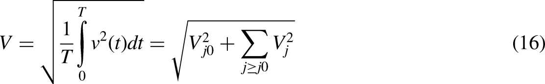
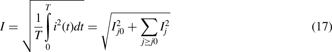
The frequency domain technique may offer information on the amplitude-frequency spectrum, but it does so at the expense of information relating to time. To get over this constraint in time, frequency-based methods are being developed to specify power amounts and quality parameters by using WT. This is similar to one of the key characteristics of TQWT, which is the ability to identify transients and harmonics. Equations (16) and (17) may be used to express the RMS value of the high-frequency harmonic in the suggested research.

V = \sqrt{\frac{1}{T} \int_{0}^{T} v^{2} (t) d t} = \sqrt{V_{j 0}^{2} + \sum_{j \geq j 0} V_{j}^{2}}

(16)

I = \sqrt{\frac{1}{T} \int_{0}^{T} i^{2} (t) d t} = \sqrt{I_{j 0}^{2} + \sum_{j \geq j 0} I_{j}^{2}}

(17)

where j = 1,2,.…10 in Equations (16) and (17) means the order figure of indication cycles. The models in one cycle are embodied as T. V and I embody the sampled vital signal achieved with the tender of TQWT. Here, Vj and Ij look like the harmonic signal attitude of all frequency components of 350 Hz and above.

Calculation of entropy

An Entropy provides information about the uncertainty related to the signal and its quantity. Thus, it can be understood that any information related to the signal defect can be obtained based on the entropy measurements. Entropy is defined as the degree to which disorder exists and it begins with a wavelet energy calculation. The arc voltage property can be reflected from the energy entropy E_i as in Equation (18) (Nir et al., 2020).

E_{i} = | C_{i} (t) |^{2}

(18)

In Equation (18), C_i(t) denotes the high-frequency coefficients components of the TQWT extracted arc V, and i denotes the count of the taking out stages. In this proposed approach, the energy distribution may be mathematically stated as the relation between the overall energy and the energy of the subband signal can be defined as the ratio of the total energies in Equation (19):

P_{i} = \frac{E_{i}}{E}, E = \sum_{i = 1}^{n} E_{i}

(19)

The normalized spectral entropy of a signal relayed on WT theory can be represented as in Equation (20).

E_{Spectral} = - \sum_{m = 1}^{N} P_{i} \log_{2} (P_{i})

(20)

For normalizations, the entropy numbers are measured in a range of 0 to 1. The normalization has been represented in Equation (21), where N is the frequency points or one-half the time series’ duration, whichever comes first.

E_{Normalized} = \frac{E_{Spectral}}{\log_{2} (N)}

(21)

The determination of the best possible number of levels of decomposition

The nonnormalized version of Shanon's entropy has been included in this paper so that the appropriate degree of decomposition or error signal may be selected. To get the most performance out of a good mother wavelet and to limit the amount of computing complexity involved, one of the most critical criteria is the selection of the optimal level. The amount of randomness included inside a voltage signal.

y_{n} = (y_{0}, y_{1}, \dots ., y_{n - 1})

(22)

D (y) = - \sum_{n}^{n - 1} | y_{n} |^{2} \ln | y_{n} |^{2}

(23)

The computation of entropy at each level of the decomposition is used to identify which degree of decomposition is the most effective. In the event that there exists a new j such that:

J (y)_{j} > J (y)_{j - 1}

(24)

Then the level j is omitted.

Selection of decomposition level and mother wavelet

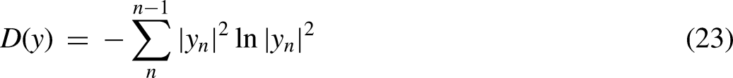
In the proposed work of the fault detection approach, the goal is to select an appropriate decomposition level after decomposing the signal into a specific number of levels. K as the statistical feature (Zhao and Li, 2017), has been used to select the best decomposition level. The shape of the probability distribution is portrayed by K. K measures the peaks of the signal and that is the most sensitive characteristic to detect the presence of disturbances. K measures the deviation from the mean of the probability density function of a random signal x(t) (Valenza et al., 2013). Therefore, it can be concluded that the level having the highest K value bears the highest deviation from its mean. This enables the extraction of more abundant fault features from the mode with the highest K value. The K values for all levels are calculated and represented in Table 1. The K is represented by Equation (25):

K = \frac{E {(x - μ)}^{4}}{σ^{4}}

(25)

Table 1.

Mother wavelet and decomposition degree selection.

Fundamental wavelet	Decomposition level	K (without noise)	K (without noise)
dB4	1	1.5 × 102	1.5 × 105
	2	1.87 × 102	1.81 × 105
	3	2.1 × 102	2.1 × 105
	4	2.03 × 102	1.91 × 105
	5	1.76 × 102	1.97 × 105
	6	1.75 × 102	1.87 × 105
	7	1.75 × 102	1.87 × 105
dB6	1	1.32 × 102	1.98 × 105
	2	1.55 × 102	2.2 × 105
	3	1.67 × 102	2.5 × 105
	4	1.74 × 102	2.67 × 105
	5	1.44 × 102	1.91 × 105
	6	1.34 × 102	1.9 × 105
	7	1.34 × 102	1.9 × 105
dB8	1	1.43 × 102	1.78 × 105
	2	1.56 × 102	1.9 × 105
	3	1.62 × 102	2.5 × 105
	4	1.76 × 102	2.65 × 105
	5	1.43 × 102	2.4 × 105
	6	1.4 × 102	2.3 × 105
	7	1.4 × 102	2.3 × 105
dB9	1	1.67 × 102	1.91 × 105
	2	1.77 × 102	2.1 × 105
	3	1.85 × 102	2.43 × 105
	4	1.97 × 102	2.5 × 105
	5	1.65 × 102	2.2 × 105
	6	1.65 × 102	2.1 × 105
	7	2.3 × 102	2.1 × 105
dB10	1	1.3 × 103	2.5 × 107
	2	2.09 × 103	2.8 × 107
	3	2.3 × 103	3.8 × 107
	4	2.02 × 103	4.1 × 107
	5	1.89 × 103	2.2 × 107
	6	1.85 × 103	1.8 × 107
	7	1.85 × 103	1.8 × 107

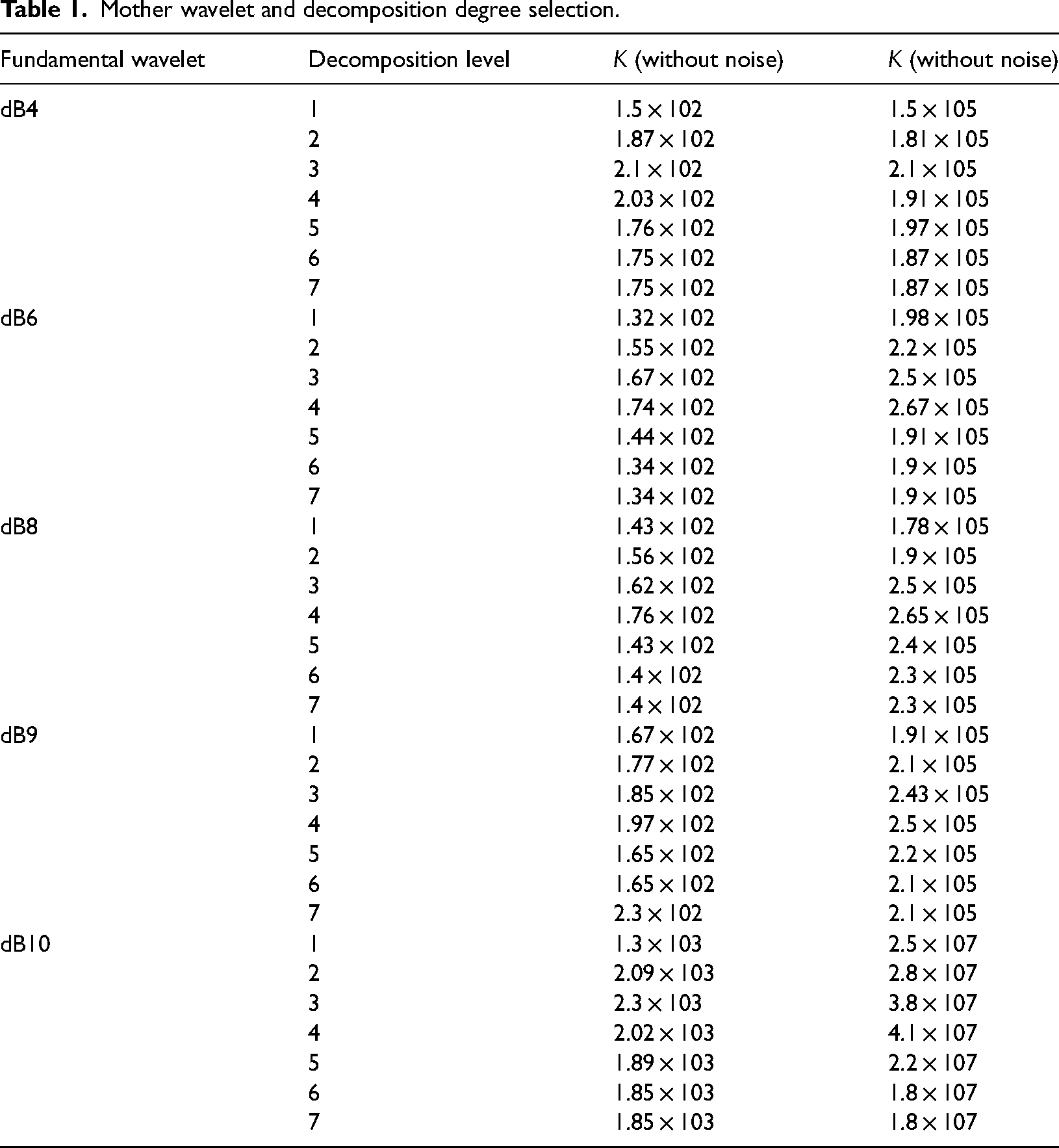
The influence of noise on the K value can also be investigated by adding 10 Gaussian noise to the current signal (Sharma et al., 2022). The existence of measurement noise in the signal does not interfere with decomposition level selection because the effect of noise on the K value is very small. The K value rises with the number of modes, and attains a maximum value of 2.3 × 103 at Level 3, then decreases further, and finally saturates at Level 5 and beyond. Therefore, for the fault detection method, the overall decomposition level is set to 5 and dB 10, which has the highest K value. This is to provide maximum data about the fault content of the signal.

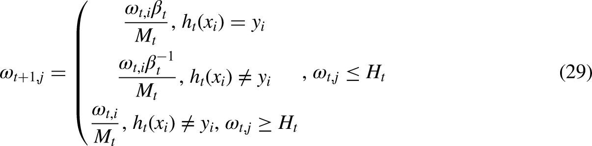
Enhanced AdaBoost machine learning classifier

To increase the speed and efficiency of the traditional AT, modified AT is predicated on two-threshold values (TVs) (Chou and Truong, 2021). The study by (Chou and Truong, 2021) also proposed an enhanced method that tackles the problem of the overbearing weight of samples at training by describing a TV that combines whether the sample is mistakenly categorized and whether the present weight value is higher than the TV. These improvements in the estimate of categorization errors and weight adjustments are made by (Chou and Truong, 2021): (1) The two-threshold exploring technique proposed in the paper is used to determine the two TVs of the two-threshold classifier. Applying the sample classification, the weighted error rate associated with the weak classifier is computed, as indicated by Equation (26):

ε_{j} = \sum_{i = 1}^{n} ω_{t, i} | h_{j} (x_{i}) - y_{i} |

(26)

h_{j} (x) = (\begin{matrix} 0, others \\ 1 \end{matrix} g_{j} (x) ε [{θ_{j}}^{(1)}, θ_{j}^{(2)}]

(27)

Setting the training weight for this round to updating the TV is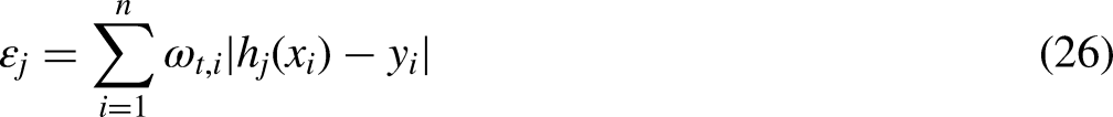

H_{t} = \sum_{t = 1}^{n} \frac{ω_{i, j}}{n}

(28)

The new weight update formula is as follows:

ω_{t + 1, j} = (\begin{matrix} \frac{ω_{t, i} β_{t}}{M_{t}}, h_{t} (x_{i}) = y_{i} \\ \frac{ω_{t, i} β_{t}^{- 1}}{M_{t}}, h_{t} (x_{i}) \neq y_{i} \\ \frac{ω_{t, i}}{M_{t}}, h_{t} (x_{i}) \neq y_{i}, ω_{t, j} \geq H_{t} \end{matrix}, ω_{t, j} \leq H_{t}

(29)

where

β_{t} = \frac{ε_{t}}{1 - ε_{t}}, M_{t} = \sum_{i = 1}^{n} ω_{t, i}

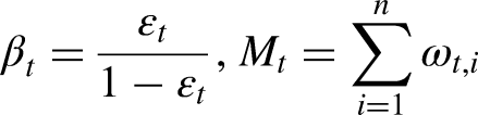
Optimal location selection of smart meters (SMs) using Jellyfish Optimizer (JFO)

It is necessary to install SMs to detect the defect in the distribution line, which can then determine what the problem is. It is possible to lower the total cost of installation by cutting down on the quantity of fault detectors. A crucial optimization plan must be put into place to reduce the number of SMs and pinpoint the location that would be best for one of these units (Every et al., 2017). The JFO is used to locate the SM in the most advantageous location possible (Chou and Truong, 2021). The equation that describes the objective function of the optimal location problematic is as follows:

Minimize $\sum_{g = 1}^{k} H_{g}$ (30) Subjected to $[X] * [H] \geq [b]$

where X resembles a connectivity matrix, and k denotes the number of buses. [X] can be represented as in Equation (31):

Matrix X_{m n} = {\begin{matrix} 1, i f m = n \\ 1, i f m and n are connected \\ 0, i f apart \end{matrix}

(31)

whereas b resembles a column matrix, and

[b] = [11111 \dots . .1]_{1 X N}^{T}

JFO technique

One of the most recent examples of metaheuristic optimization algorithms, known as the JFO, was created in the year 2020 by J-S Chou and D-N Truong (Chou and Truong, 2021). The behavioral process that jellyfish use to look for their food in the moving ocean current served as the basis for the JSO’s overall structure as an organization. The JFO’s implementation is controlled by three fundamental features of the jellyfish’s behavior, which are as follows: The jellyfish travels with the currents of the water or forms associations among swarms to facilitate its migration. A time control mechanism is in charge of directing the transition that takes place between these two motions. When the jellyfish swim about in quest of food, they are eventually drawn to the area that has the greatest quantity of food. This process draws them to the location where there is the most food. While calculating the total quantity of food that was followed by the JFO throughout its journey, it is important to take into account both the location of the JFO as well as its objective purpose. A time control system is in charge of deciding when to transition between these two different motions.

Ocean current

Jellyfish are drawn to the direction of the ocean current because it has an abundance of nutrients that are readily available. The direction of the ocean current is determined After determining which jellyfish is at the best place, in this study utilization the mean of the vectors acquired from all of them, which may be symbolized as Equations (32) and (33). In other words, the direction of the ocean current is determined by the average value of the vectors.

\vec{Trend} = \frac{1}{{Num}_{pop}} \sum {\vec{Trend}}_{i} = \frac{1}{{Num}_{pop}} \sum (H^{*} - g_{c} H_{i}) = H^{*} - g_{c} \frac{\sum H_{i}}{{Num}_{pop}} = H^{*} - g_{c} μ_{s}

(32)

\vec{Trend} = H^{*} - d f

(33)

Set df = g_cµ_s

It can be seen from Equation (32) that the inhabitants of jellyfish treated to be as NUM_pop, H* that represents the jellyfish’s current fit location, µ_s that looks like where found the jellyfish to be on average, g_c that is the factor that governs the attraction, and df that represents the difference between the most recent best jellyfish position and the determined mean position of all of the jellyfish.

In order to take into consideration, the way that jellyfish are distributed around the ocean, it has been assumed that they have a regular spatial distribution. As a result, a distance ± Y_sɕ_s of has been regarded to be within the immediate neighborhood of the specified average location having the probability for the existence of all jellyfish, ɕ where denotes the standard deviation that has been supported for the spatial distribution. Equation (34) is a mathematical expression that may be used to describe something.

d f = γ_{s} \times σ_{s} \times Random (0, 1)

(34)

Set

σ_{s} = Random (0, 1) \times μ_{s}

(35)

Hence,

d f = γ_{s} \times σ_{s} \times Random (0, 1) \times Random (0, 1) \times μ_{s}

(36)

So, taking into account the aforementioned mathematical expressions, the Equation (36) may be expressed more straightforwardly as follows:

d f = γ_{s} \times μ_{s} \times Random (0, 1)

(37)

where,

g_{c} = γ_{s} \times Random (0, 1)

(38)

Thus,

\vec{Trend} = H^{*} - γ_{s} \times Random (0, 1) \times μ_{s}

(39)

The most recent positional updates position of jellyfish may be expressed by the following:

H_{i} (k + 1) = H_{i} (k) + Random (0, 1) \times \vec{Trend}

(40)

Likely, Equation (40) is expressed as:

H_{i} (k + 1) = H_{i} (k) + Random (0, 1) \times H^{*} - γ_{s} \times Random (0, 1) \times μ_{s}

(41)

Equation (41), Y_s denotes the specified coefficient distribution, and the value Y_s = 3 was determined based on the results of the 30 separate trials conducted independently of one another.

Swarming occurrence of Jellyfish

There are two types of motion that the jellyfish swarm displays in the ocean currents: passive movement and active movement. The majority of the jellyfish exhibited a movement type referred to as active during the early phases of the creation of the swarm; however, as the formation continued for a longer period of time, the jellyfish shifted their motion from active to passive. In the situation when the jellyfish is moving in an active motion, the motion that it is maintaining is around its group, and the position update for this scenario may be found by using Equation (42):

H_{i} (k + 1) = H_{i} (k) + ξ_{s} \times Random (0, 1) \times (U_{B} - L_{B})

(42)

being U_B and L_B respectively, the search space's upper and lower bounds. ξs > 0 is analogous to the motion coefficient that controls the path taken by the jellyfish. At the beginning of the passive, a jellyfish is chosen at random. This jellyfish must be unique in comparison to the jellyfish that is being studied (Jf_j). Using a vector that extends from to, one may calculate the path that the motion will take (Jf_j). If there is more food at the place if the distance between the two is more than the distance between the two the jellyfish will go in that direction. On the other hand, if the extent of the food that is available at the position is less than what is available at the position, then travels in the opposite direction of the movement of (Jf_j). Because of this activity, the jellyfish can shift into a position that is more advantageous for it to look for food. Jellyfish can efficiently utilize the search space because of a behavior known as traversal, which may be mathematically described in Equation (43):

\vec{Step =} H_{i} (k + 1) + H_{i} (k)

(43)

where,

\vec{Step =} Random (0, 1) \times \vec{Direction}

(44)

\vec{Direction} = {\begin{matrix} H_{j} (k) - Z_{i} (k) i f f (H_{i}) \geq f (H) \\ H_{i} (k) - Z_{j} (k) i f f (H_{i}) < f (H) \end{matrix}

(45)

when there is a function that is similar to the aim, as well as a place that is similar to the jellyfish. The equation that represents the most recent location of the jellyfish may be found here.

H_{i} (k + 1) = H_{i} (k) + \vec{Step}

(46)

Time control mechanism

For the whole of the JFO’s execution, a time control system has been implemented in order to distinguish between the various types of motion. Not only does it control the movements of type A and type B swarms, but it also controls the movements of jellyfish in the direction of the ocean current.

Since it carries huge quantities of food, jellyfish are naturally attracted to the direction that the ocean current is moving in. Over the course of time, more and more jellyfish will gather together, eventually becoming a swarm. When there is a change in the temperature or wind factors, the jellyfish move into a different ocean current. This ultimately leads to the birth of another jellyfish swarm. The motions of a swarm of jellyfish may be broken down into two categories: active and passive motions. The jellyfish switch back and forth between the two categories. At the beginning, the passive motion is selected; later on, as more time passes, the active motion is integrated into the framework. The time control TC(K) mechanism was implemented so that this situation might be reproduced in C₀. The time control approach integrates a time control function and a constant to guide the traversal behavior of the jellyfish between following the direction of the ocean current and migrating within the swarm. This allows the jellyfish to switch between the two modes with precision. In this TC(K) ɛ [0,1] context, and C₀ is denoted by the value 0.5. When the process of JSO is being carried out, the value of is contrasted with the value of. If the value of TC(K) is greater than zero, the behavior of the inhabitant jellyfish is determined through ocean current; alternatively, if the value of C₀ is less than zero, the jellyfish moves about inside its own swarm. The temporal control function can be mathematically modeled using the TC(K) < C0 Equation, which means being Maxiter denotes the maximum iteration, while K is the number of iterations.

TC (k) = | (1 - \frac{k}{{Max}_{iter}}) \times [2 \times Random (0, 1) - 1] |

(47)

The beginning stages of the inhabitants of jellies

JSO uses a randomization process to carry out the process of population initialization. The inability to attract a diverse enough population is one of the weaknesses of this approach, which also contributes to the strategy’s tendency to converge more slowly than expected and to become stuck in a cycle of reaching only locally optimal solutions. So, the diversity of the starting population has been improved as a result of the development of a few different heat maps, a few are the logistic map, the tent map, and the final Liebovitch heat map. The logistic heat map, which had been established by the month of May, was implemented in order to produce inhabitants that are more varied than those generated by random selection and to eliminate the possibility of early convergence.

H_{k + 1} = η_{s} H_{k} (1 - H_{k}), 0 \leq H_{0} \leq 1

(48)

where Equation (48), H_k encapsulates the position's logistically chaotic worth for Kth jellyfish, η_s is defined as the number 4.0, and H₀ leads to an increase in the number of jellyfish in an area H₀ ɛ (0,1).

Boundary condition

There are oceans all across the surface of the world. Since the planet has a nearly spherical shape, a jellyfish that strays beyond the restricted search zone will ultimately find its way back to the opposite border. The equation that describes this reentering occurrence is as follows: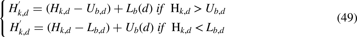

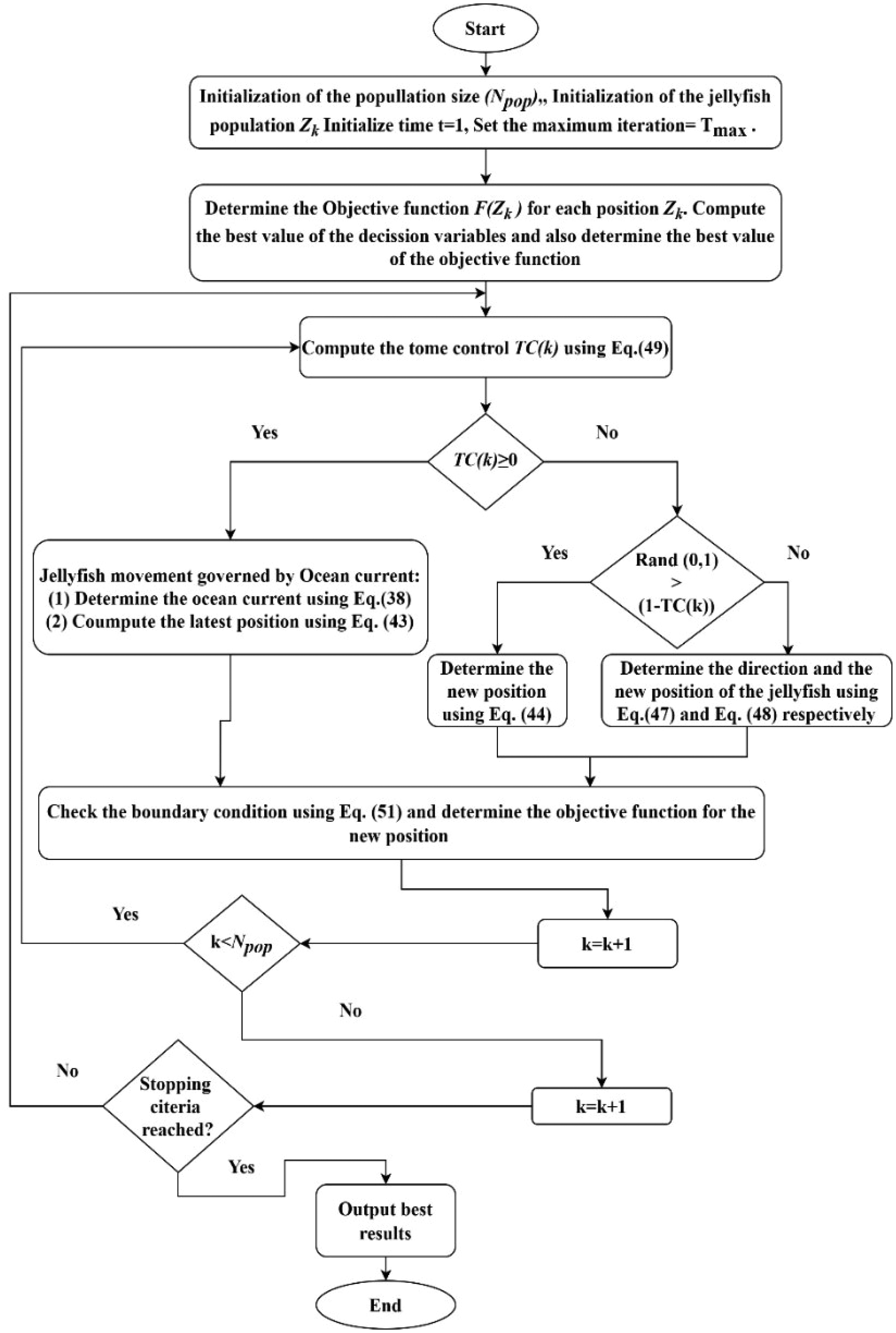
{\begin{matrix} H_{k, d}^{'} = (H_{k, d} - U_{b, d}) + L_{b} (d) i f H_{k, d} > U_{b, d} \\ H_{k, d}^{'} = (H_{k, d} - L_{b, d}) + U_{b} (d) i f H_{k, d} < L_{b, d} \end{matrix}

(49)

where in Equation (49), the location of the jellyfish is indicated for the dimension as Kth, Z_k,d if this is the updated position post, then the boundary limitations of the search region have been verified. The top limit of the search space for dimension is denoted by, whereas the lower limit is denoted by U_b,d, and L_b,d The jellyfish optimization approach for the optimum placement of SMs is depicted here in the form of a block diagram in Figure 2.

Figure 2.

The JFO flowchart for precisely inserting SMs.

Graph Search Technique for Partitioning Off Protective Zones

The topology of the power system makes use of vertices (V) and edges (E), both of which are topologies from the field of graph theory. These guidelines are outlined in further detail in reference (Joga et al., 2021a). For the purpose of zone separation, the following rules are currently being considered:

Rule 1: A new protection zone will be produced an original Bus is introduced together with the existing guard zone by a vertex. This will cause the formation of a new protection zone.

Rule 2 stipulates that if the protection zone contains any clones of buses, only one of them shall be maintained while the rest mirror zones should be eliminated.

These two guiding tenets are taken into consideration while solving the search problem, which entails finding the optimal location for the SM inside the protection zone. On the basis of the aforementioned two guidelines, a one-of-a-kind protection approach was provided. The stages of the method that are mentioned below have been validated for use on an IEEE 33-bus system, and the same validation process has been carried out for an IEEE 123-bus system. The procedures involved are shown in Figure 3. The first step involves managing each of the basic buses in an initial zone. This happens in the first stage. For instance, bus 1 is considered a zone under the IEEE 33 testing system.

Figure 3.

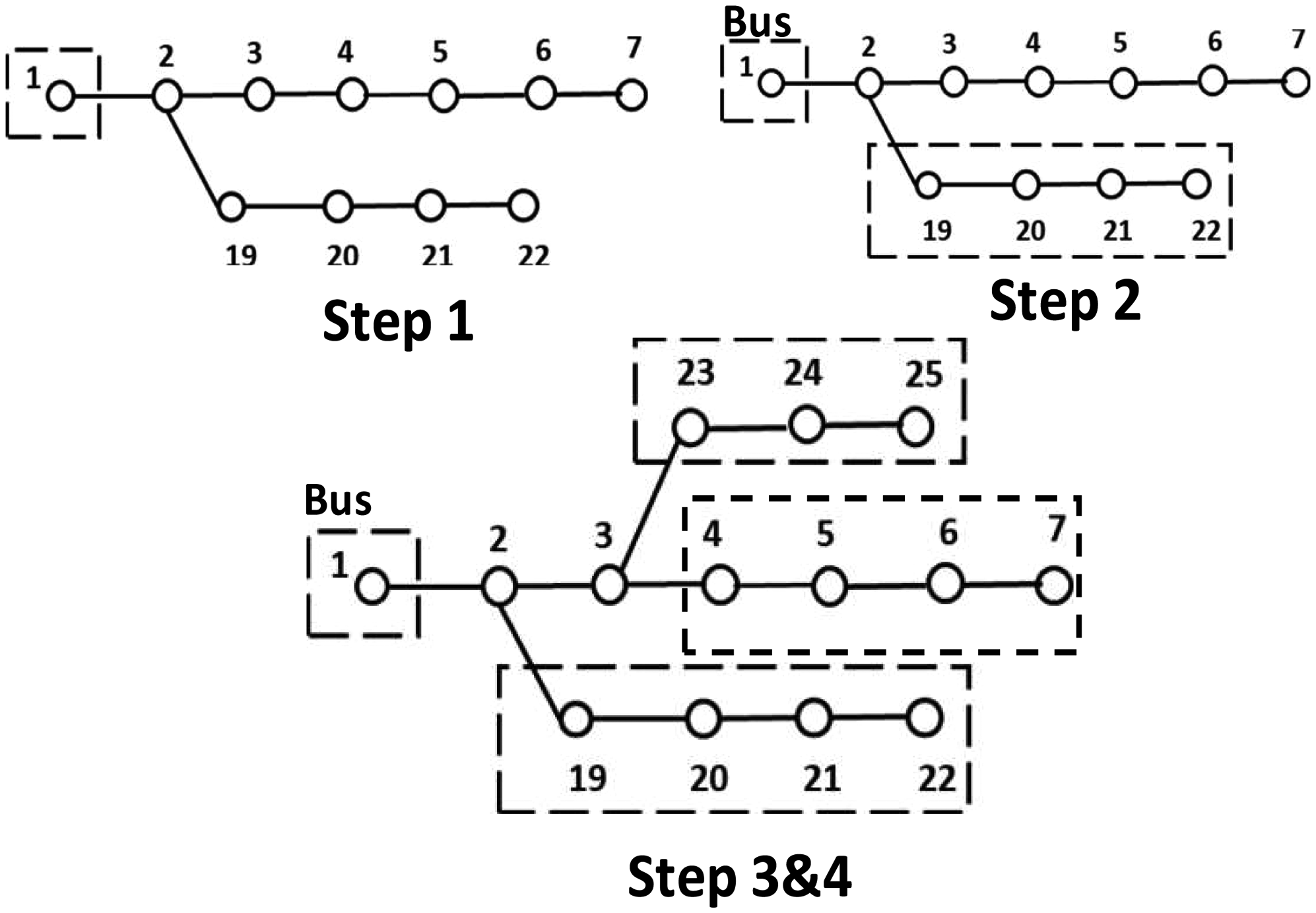
Suggested graph search method steps.

Second Step: At this step, the initial bus looks for other buses in the immediate area and joins forces with them all to create an alternate zone.

In the third step of the process, the search criteria include doing a comparison between the old zone and the new zone established in the second step. So, in the event that there are any buses that are equivalent to the ones being protected, this area (zone) will be eliminated so that all buses may be protected in the same manner.

The last step of the search process is when the search algorithm checks to check whether the sum of the buses in the zone and the network is equal. If this is the case, the search process is finished, and if it is not, the algorithm moves on to Step 2.

Results and discussions

Using the IEEE 33- and IEEE 123-bus systems, an evaluation is conducted on the technique that is recommended. Both Meera and Hemamalini (2017) and Marcos et al. (2017) provide information that is relevant to the IEEE 123- and the IEEE 33-bus system, respectively. Figure 4 illustrates the most advantageous position for the positioning of the measurement devices in relation to the use of JFO. It has been determined that the sample duration is 0.0997 milliseconds, which is equivalent to a sampling frequency of 10.025 kHz. As a result, the sampling frequency for the TQWT method has been determined to be 10.025 kHz. Together with the sampling frequency, the sample size has been an important factor to consider in this study that has been recommended. The total number of samples is 1024, and they were taken throughout the course of 20 cycles here.

Figure 4.

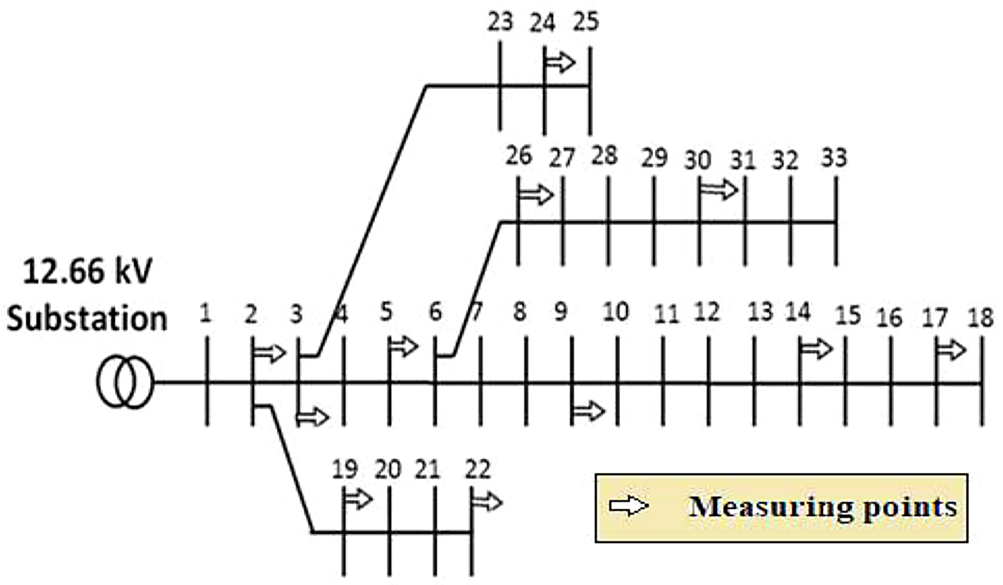
IEEE 33-bus system one-line diagram.

Figure 5 shows the implementation scheme of the proposed method. In such a scheme, meters are installed along the PDS, and data concentrators connect the data to the red box. The HIF scheme is shown with four function blocks: feature extraction and selection, TQWT-based HIF detection, zone-wise HIF location identification, and HIF execution.

Figure 5.

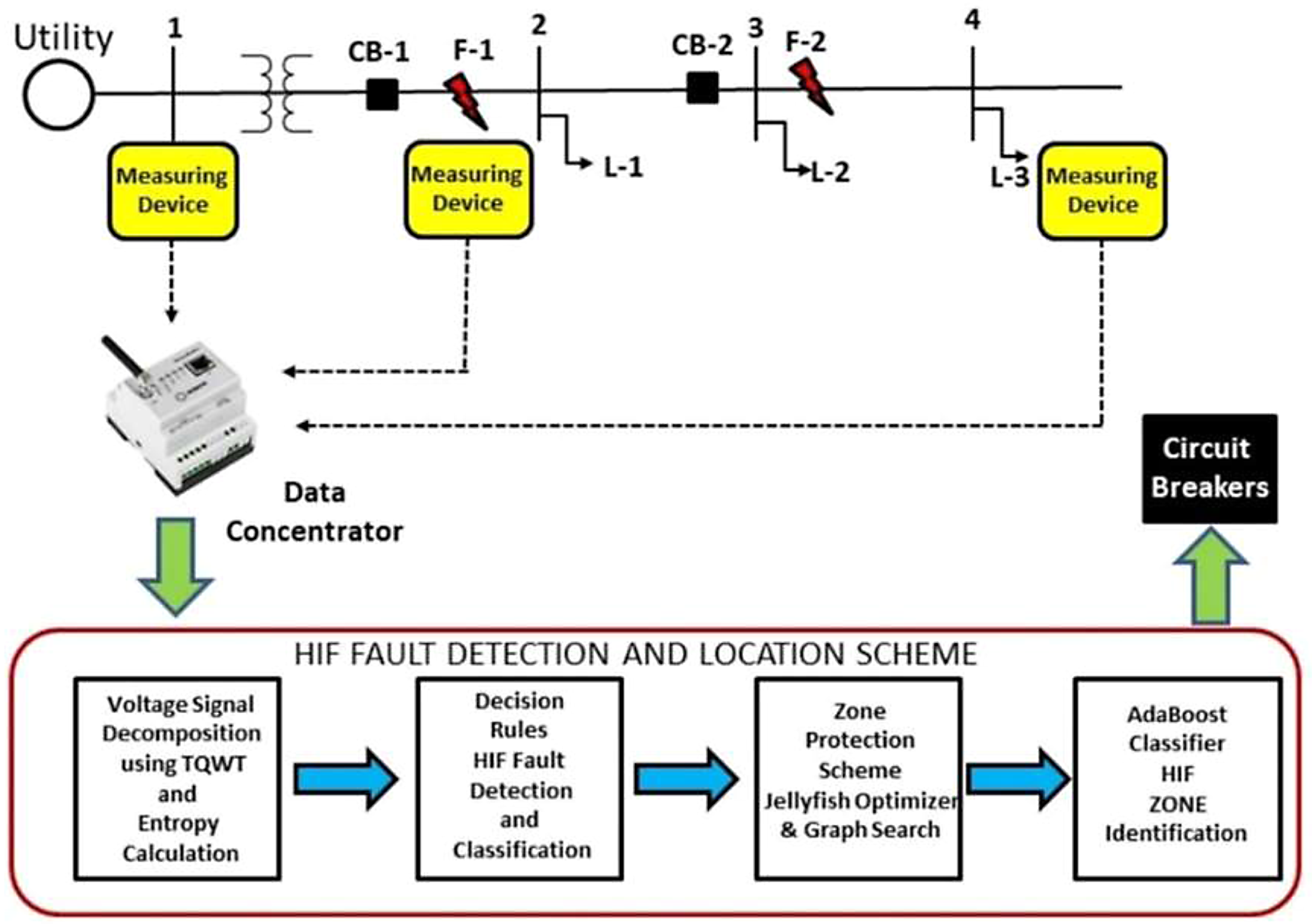
Functional block diagram of proposed HIF detection scheme.

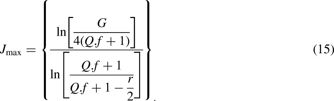
A two-stage proposed procedure has been represented in Figure 6 to detect, classify, and locate the zone of HIF in PDSs. In the first stage, healthier and fault signals that are collected from optimally placed meters are analyzed through TQWT using Equations (16) and (17). The decomposition level j depends on the total of the dominant-frequency components of the input signal and the value of j should preferably be smaller than its maximum, that is, Jmax which is shown in Equation (15). A smaller j initiates the aliasing of different components and a larger j creates a high computational burden (Yang et al., 2022). The correct approach for selecting the appropriate decomposition level and mother wavelet is presented in Table 1.

Figure 6.

The proposed method structure.

In Figures 7 and 8, the TQWT decomposition level and generated harmonics are shown respectively. As per Figure 8, up to 13th-order harmonics are the most dominating in the case of HIF fault. So up to seven levels of decomposing have been done but based on the K value concept up to the fourth level of decomposition has been chosen as this one is the most optimum level because up to this level, the K value increases after that it's decreasing which means at Level 4 maximum harmonic related information can be extracted. Third level of decomposition may create an aliasing problem and up to the seventh level of decomposition creates a computational burden. Following the determination of j, r, and Q are chosen to guarantee that the main and deviated components of the input signal are precisely extracted. This is done because the fundamental component, which has a frequency of 50 Hz, is necessary to choose appropriate r and Q values for a variety of PQD signals.

Figure 7.

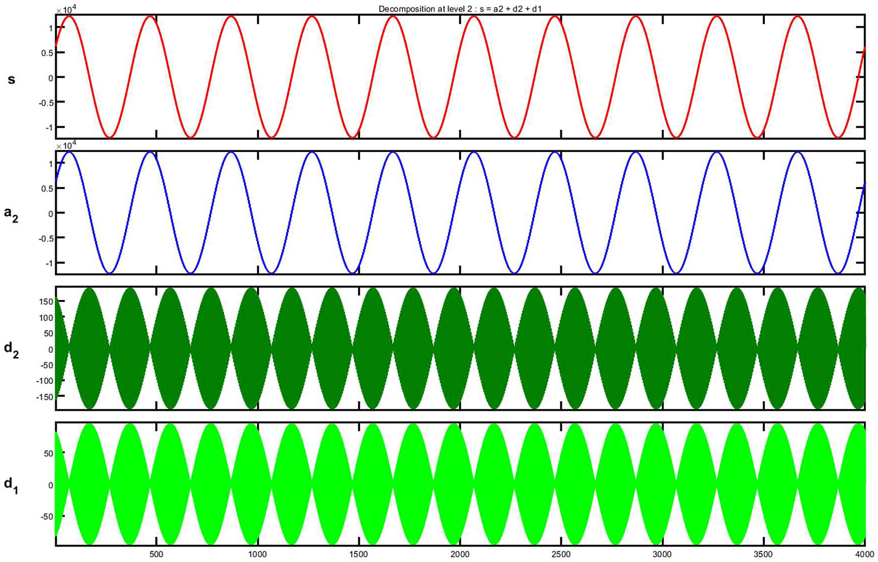
TQWT decomposition of faulted signal up to Level 2 of the voltage signal.

Figure 8.

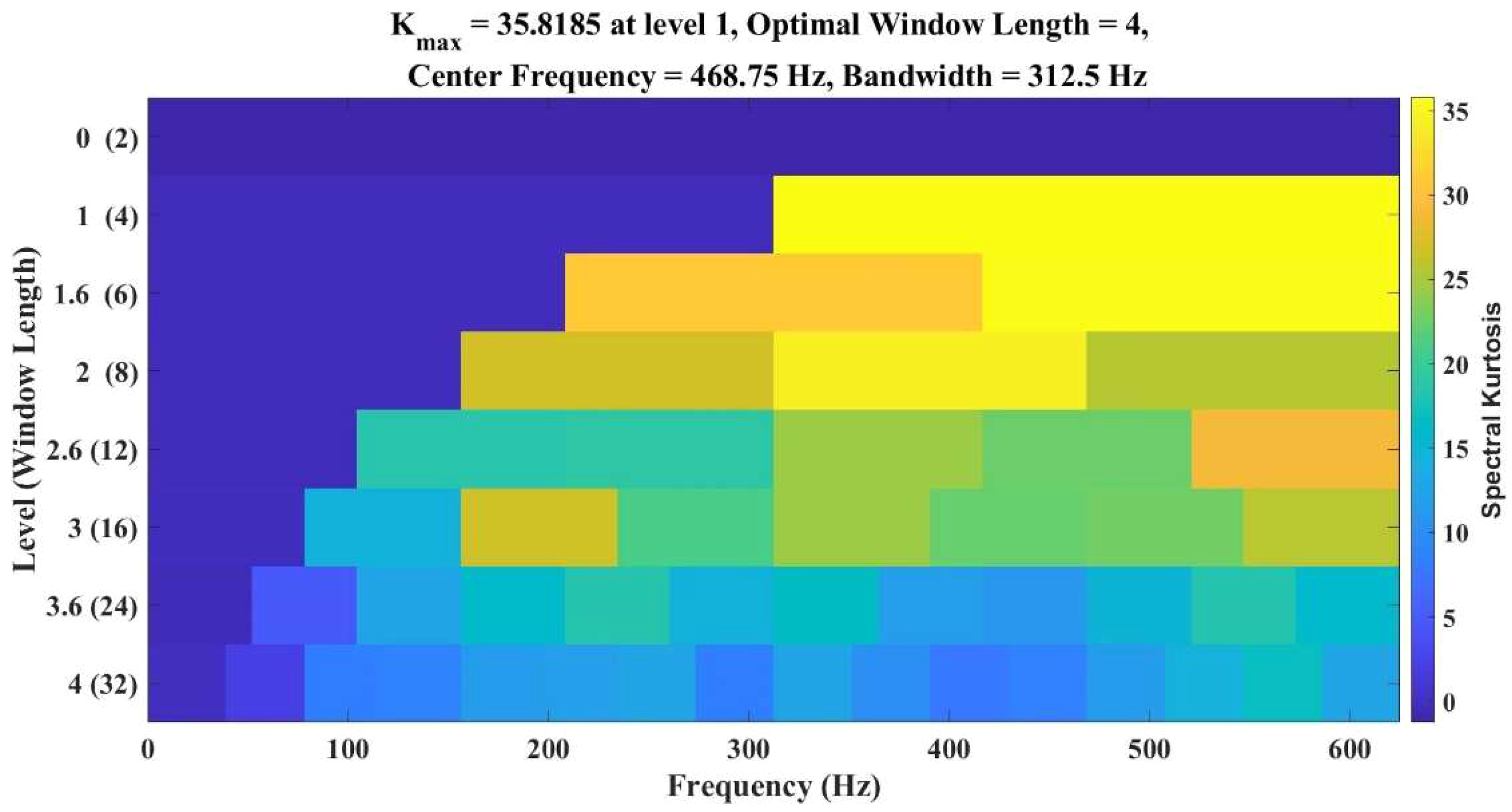
Kourtogram of generated harmonics during HIF fault in the voltage signal.

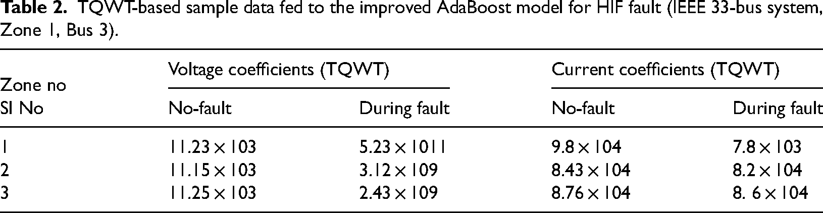
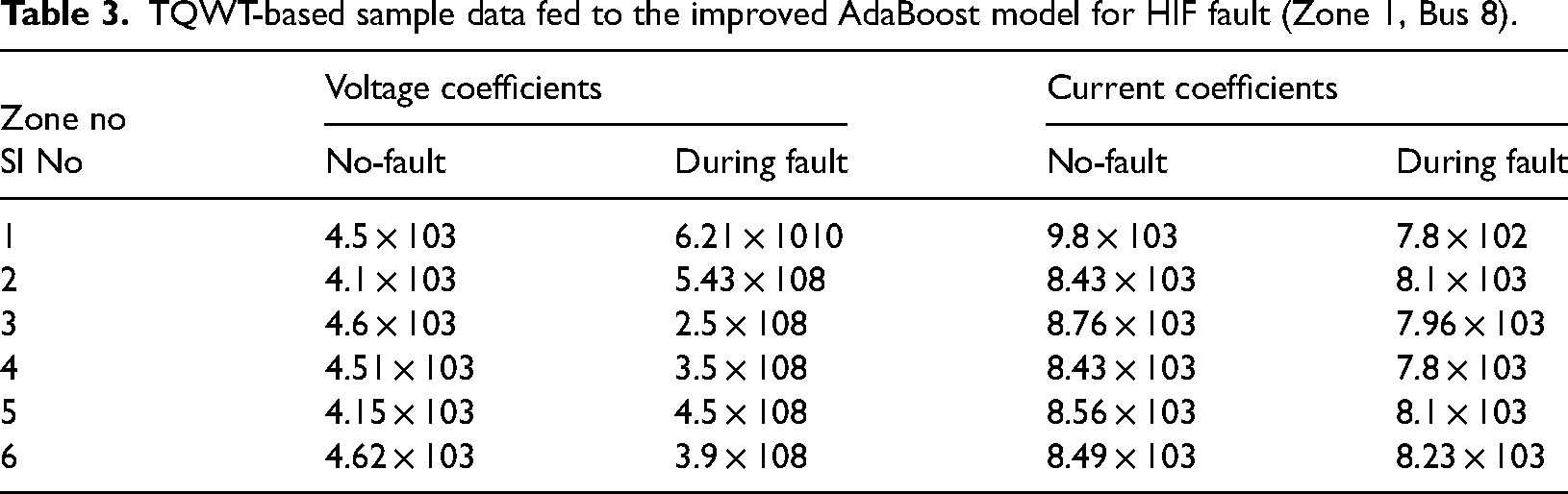
Tables 2 and 3, show that TQWT generated some of the voltage and current coefficients which are fed to the improved AdaBoost classifier to train the model for IEEE 33- and 123-bus systems respectively. It can be observed from these two tables that, in faulted (HIF) bus voltage coefficients are quite high rather than in healthy conditions whereas in the case of the current coefficient, it is much less than in the healthy condition. Hence conventional relays can’t detect this type of fault.

Table 2.

TQWT-based sample data fed to the improved AdaBoost model for HIF fault (IEEE 33-bus system, Zone 1, Bus 3).

Zone no	Voltage coefficients (TQWT)		Current coefficients (TQWT)
Sl No	No-fault	During fault	No-fault	During fault
1	11.23 × 103	5.23 × 1011	9.8 × 104	7.8 × 103
2	11.15 × 103	3.12 × 109	8.43 × 104	8.2 × 104
3	11.25 × 103	2.43 × 109	8.76 × 104	8. 6 × 104

Table 3.

TQWT-based sample data fed to the improved AdaBoost model for HIF fault (Zone 1, Bus 8).

Zone no	Voltage coefficients		Current coefficients
Sl No	No-fault	During fault	No-fault	During fault
1	4.5 × 103	6.21 × 1010	9.8 × 103	7.8 × 102
2	4.1 × 103	5.43 × 108	8.43 × 103	8.1 × 103
3	4.6 × 103	2.5 × 108	8.76 × 103	7.96 × 103
4	4.51 × 103	3.5 × 108	8.43 × 103	7.8 × 103
5	4.15 × 103	4.5 × 108	8.56 × 103	8.1 × 103
6	4.62 × 103	3.9 × 108	8.49 × 103	8.23 × 103

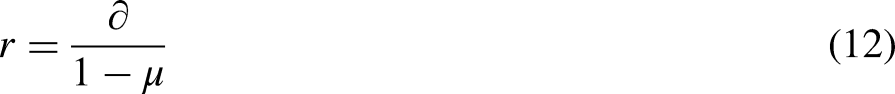
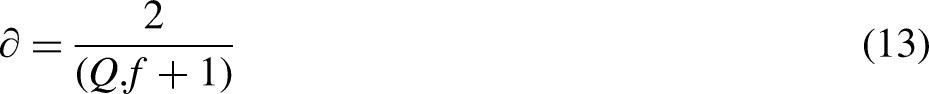
The parameter known as redundancy R is calculated by dividing the count of wavelet coefficients for the whole duration up to the input signal that is being processed by the TQWT (Reddy and Rao, 2016). As there are a total of 3072 coefficients in this system, and signal duration (in terms of sample counts), is 1024, the value of r in this context is 3. There is a correlation between the QF and the breadth of the bandpass filter. As the bandpass filter has a relatively low QF but a relatively broad passband, just a small number of levels are required to cover signal of interest spectral content. Due to the high QF that is linked with the narrow bandpass filter, there must be an increased number of levels to cover the signal's spectrum. As a result, in this approach, Q = 1 is decided upon because there are a total of five stages of decomposition, as shown in Figure 9. As per the filter specification in Equations (13) and (14), μ = 0.666 and β = 0.778, hence the value of R = 3.

Figure 9.

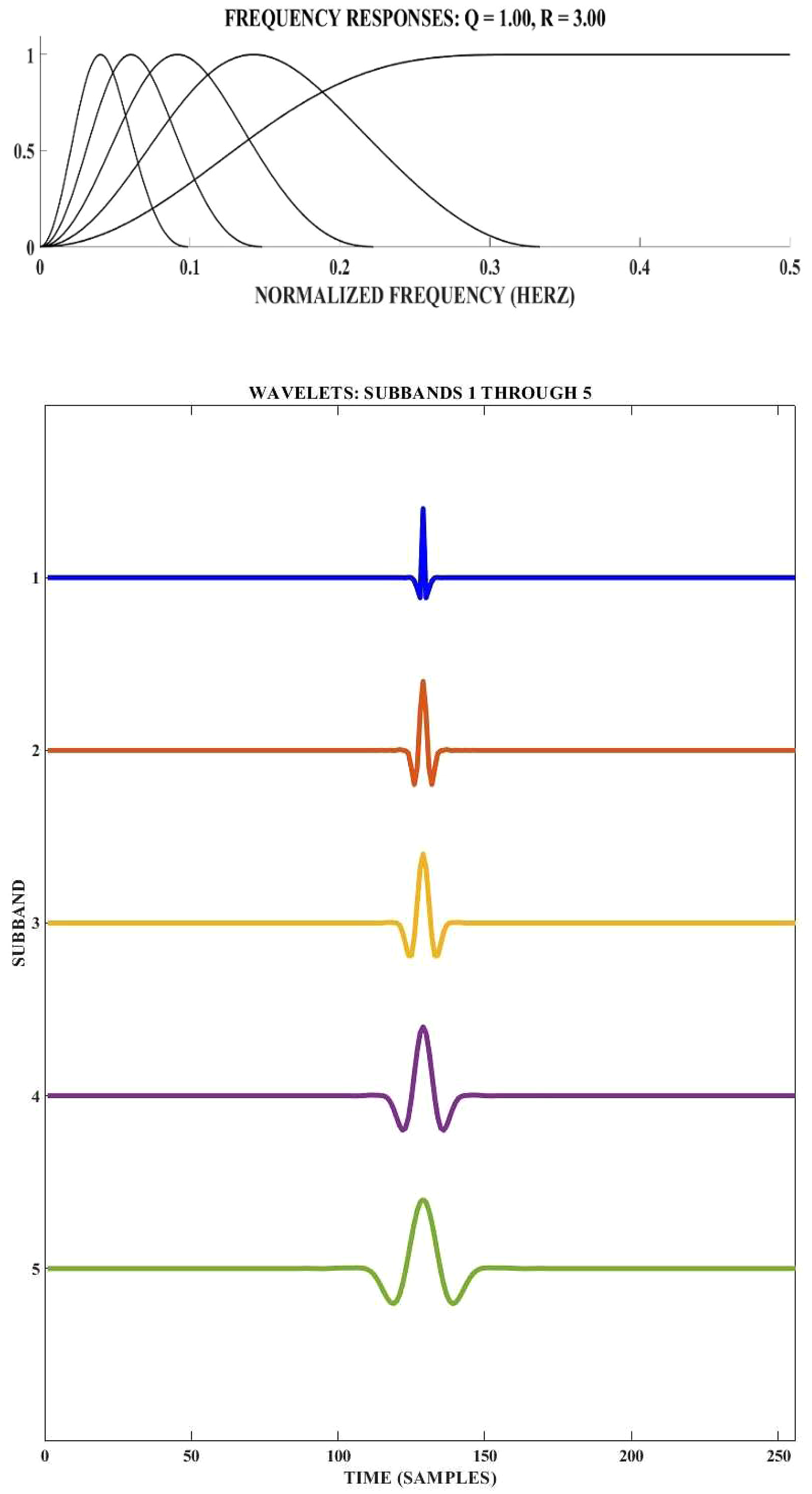
Frequency response and wavelet functions of wavelet subband of TQWT basis when Q = 1, R = 3, and J = 5: wavelet subband when Q = 1, R = 3, and J = 5.

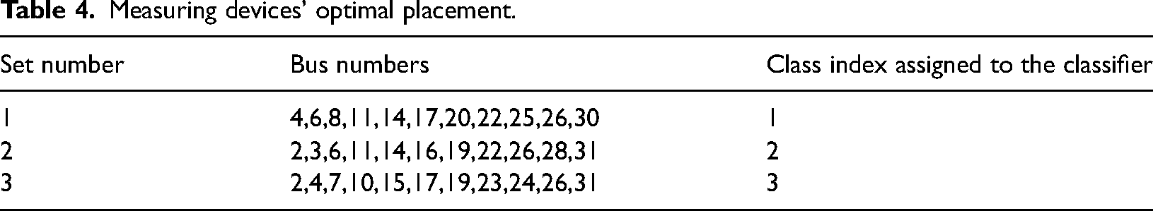
The meters are optimally placed through the JFO technique. To determine the entropy of a signal, it must be broken down into its constituent subbands. using Equations (18)–(21). The optimal solution is obtained as shown in Equation (30) and the optimal solutions are also shown in Table 4.

Table 4.

Measuring devices’ optimal placement.

Set number	Bus numbers	Class index assigned to the classifier
1	4,6,8,11,14,17,20,22,25,26,30	1
2	2,3,6,11,14,16,19,22,26,28,31	2
3	2,4,7,10,15,17,19,23,24,26,31	3

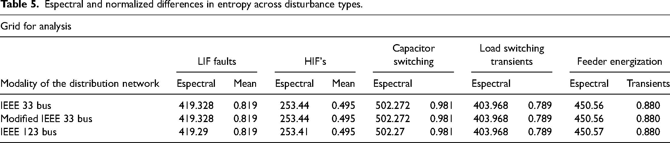
Values are used to determine the criteria for making decisions calculated by the mean entropy concept which are shown in Table 5 at each transient to detect and categorize HIF from low-impedance faults. Subsequently, a new zone protection outline is projected considering the concept of the graph. This strategy partitions a distribution network into zones, isolating the problematic area from the rest of the network. AdaBoost machine learning classifier is implemented to detect the zone of fault.

Table 5.

Espectral and normalized differences in entropy across disturbance types.

Grid for analysis
Modality of the distribution network	LIF faults		HIF's		Capacitor switching		Load switching transients		Feeder energization
Modality of the distribution network	Espectral	Mean	Espectral	Mean	Espectral		Espectral		Espectral	Transients
IEEE 33 bus	419.328	0.819	253.44	0.495	502.272	0.981	403.968	0.789	450.56	0.880
Modified IEEE 33 bus	419.328	0.819	253.44	0.495	502.272	0.981	403.968	0.789	450.56	0.880
IEEE 123 bus	419.29	0.819	253.41	0.495	502.27	0.981	403.968	0.789	450.57	0.880

The research work has been validated on the IEEE 33- and 123-bus unbalanced PDS. This section presents the HIF detection results using TQWT at different operating conditions. Different DG and noisy configurations are considered to verify the methods. The modeling and simulation are performed in MATLAB/SIMULINK and also verified in the real-time system using RTDS. In this section for the validation of the proposed method below mentioned case studies are considered.

Case 1: Shown the best mother wavelet and decomposition level to make this process faster

Case 2: Determine the optimal measuring position of the IEEE 33-bus system

Case 3: Calculation of normalized entropy for IEEE 33- and 123-bus system.

Case 4: Divide the zone of the IEEE 33-bus system based on the Graph Theory based concept

Case 5: Creating HIF faults in different buses and checking the accuracy level

Case 6: Verification of the method in IEEE 123 unbalanced network

Case 7: Evaluation of the proposed method using RTDS

A. Case 1: The best mother wavelet and decomposition level

K values have been used to select the suitable mother wavelet and the number of decomposition levels in TQWT to reduce the computational complexity which will make the process faster based on Equation (25) First K value for each level for a particular wavelet has been calculated using the Equation (25) and selected the optimum decomposition level. In this HIF fault analysis, dB10 with Level 4 is selected to be optimal to make it a faster one as it shows the highest value in Table 1.1 which signifies the combination of dB10 and fourth level of decomposition can extract the maximum features of HIF fault. Hence in this methodology, dB10 is used as the mother wavelet, and signals are decomposed up to level 4.

B. Case 2: Determine the optimal measuring position of the IEEE 33-bus system

In the distribution system, connection of measuring devices to each bus is not possible concerning the cost. So optimal placement of meters is essential to make the system observable and robust. To reduce the number of measuring devices in IEEE 33-radial distribution systems JFO techniques have been chosen. The optimal locations have been considered according to the results of thirty separate experiments of JSO. It is tabulated in Table 2.

C. Case 3: Calculation of normalized entropy

The various PQD are represented by their respective mean or normalized entropy values in Table 3, which is based on Equations (18)–(21). For the purposes of this study, normalized data have been selected to use across the various distribution networks. Through a comprehensive series of studies, it was determined that these values for the normalized entropy of any distribution system are unchangeable. To discriminate between HIF and non-HIF, these numbers are used as a benchmark value. In addition to SC faults (line-ground), the research looks at feeder-energizing transients, load-switching transients, and capacitor-switching transients. Calculations of normalized entropy values are performed in a number of different grid configurations, including the normal distribution, the realistic real-time distribution, and the integrated distribution of renewable energy sources. Given that the total length of the time series is 1024, the value of N is thus 512.

The outcomes that were recorded in Table 3 are used to inform the formulation of decision rules. The following are the decision criteria for the detection and categorization of high-impedance defects as opposed to low-impedance errors:

0.2 < Entropy <0.5 = HIF

0.5 < Entropy < 1.0 = non-HIF

According to these choice guidelines, signals with entropy values that are lower than 0.2 are considered to be in better health, but values that lie between 0.2 and 0.5 are considered to have high-impedance problems. Faults with low impedance are denoted by entropy values that are greater than 0.5.

D. Case 4: Divide the zone of the IEEE 33-bus system based on the graph theory-based concept

Based on the graph theory-based concept the IEEE 33 bus has been divided into three distinguished zones represented in Table 6.

E. Case 5: Creating HIF faults in different buses and checking the accuracy level

i) Fault Occurred in the radial distribution system

Table 6.

A graph protection zone selection for IEEE’s 33-bus system using a search algorithm.

Zone number	Bus number in IEEE 33-bus system
Zone 1	1, 2, 3,19,20,21,22,23,24,25
Zone 2	4, 5, 6, 26, 27, 28, 29, 30, 31, 32, 33.
Zone 3	7, 8, 9, 10, 11, 12, 13, 14, 15, 16,17, 18

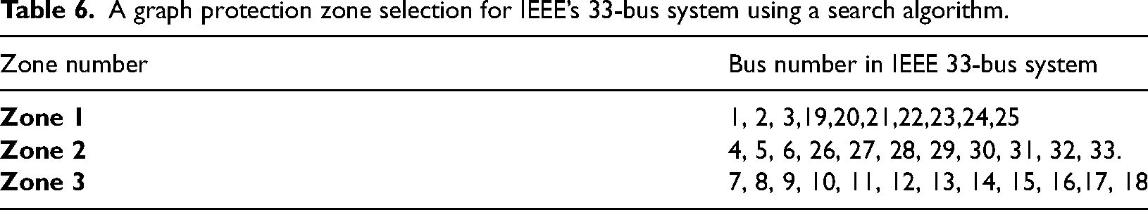
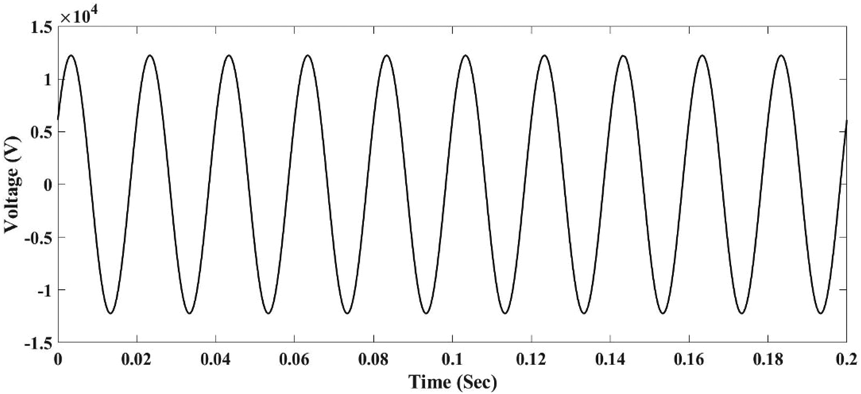
In 12.66 kV IEEE 33-bus radial distribution system is used to evaluate the proposed methodology. The Load and Bus data of the distribution system are considered (Joga et al., 2021a). In this scenario, the Arc Parameters are VP = VN = 5600 V, RP = 800 Ω, RN = 150 Ω, which form an asymmetric V-I curve. It is supposed that the line between bus 6 and 26 is subject to HIF, low-impedance fault, and other transients. The fault voltage levels and current signal levels are recorded by meters connected near the fault zone on buses 5, 26, and 30. The measured arc voltage is shown in Figures 10 and 11.

Figure 10.

Arc voltage at the location of high impedance fault.

Figure 11.

Zoom view of arc voltage at the location of high-impedance fault.

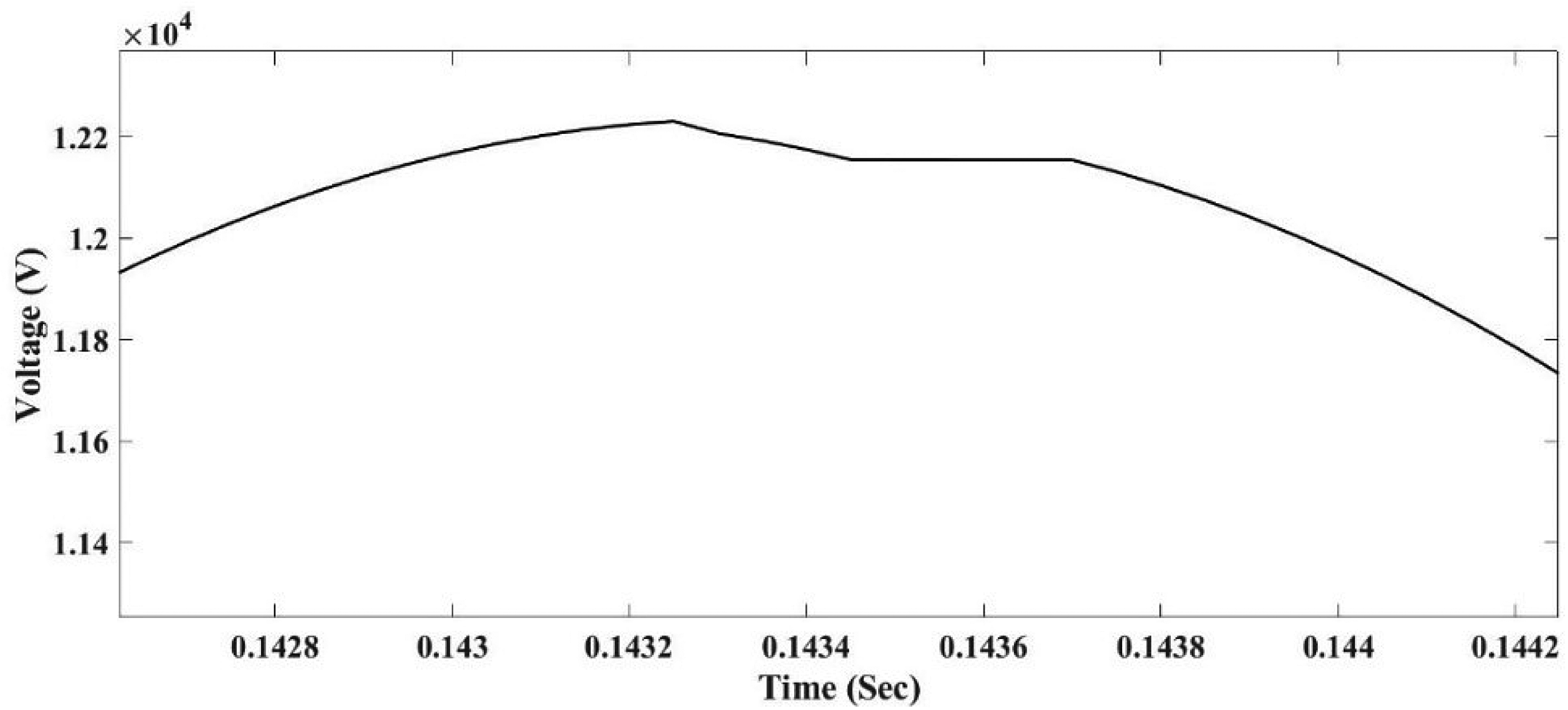
The arc voltage is further decomposed via a TQWT. The prefault data is divided into two subband levels with a QF of 1. The current waveform during an HIF is observed to be less than the line current, as shown in Figure 12.

Figure 12.

HIF current waveform at the fault location.

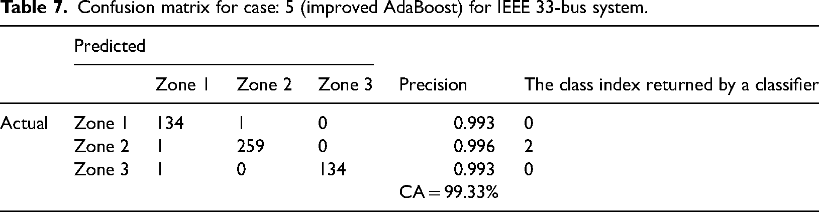
The scatter diagram visualizes the data sets in a Gaussian plane. It is drawn between Level-1 data sets to Level-2 data sets. The blue color data sets in the scatter diagram represent Zone 1, the red color data sets represent Zone 2, and the green color data sets represent Zone 3. The scatter diagram for case 5 is shown in Figure 13. It should be noted that 532 data sets have been poised from 11 fault detectors positioned across the test system. Table 7 shows the confusion matrix for Case 5. According to Table 5, 259 of the 260 fault samples are classified as Zone 2 in the confusion matrix, with a precision value of 0.99. An efficiency of 99.33% is achieved for the observed categorization task.

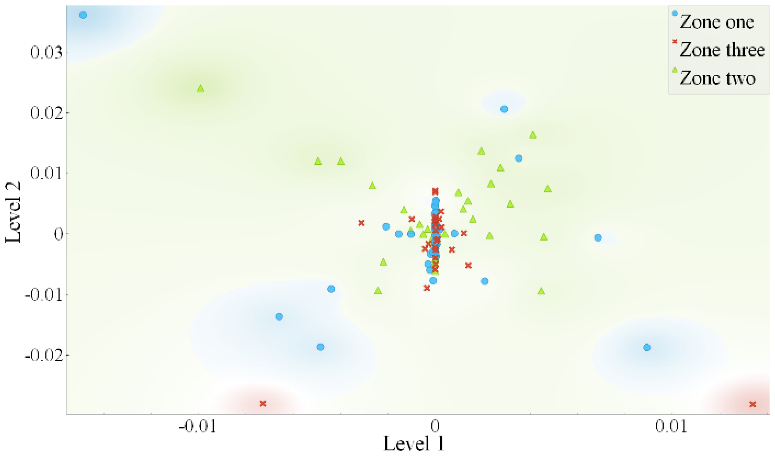
ii) Fault in another zone on IEEE 33 radial distribution system

Figure 13.

Scatter diagram for case. 5.

Table 7.

Confusion matrix for case: 5 (improved AdaBoost) for IEEE 33-bus system.

	Predicted				Precision	The class index returned by a classifier
		Zone 1	Zone 2	Zone 3	Precision	The class index returned by a classifier
Actual	Zone 1	134	1	0	0.993	0
	Zone 2	1	259	0	0.996	2
	Zone 3	1	0	134	0.993	0
					CA = 99.33%

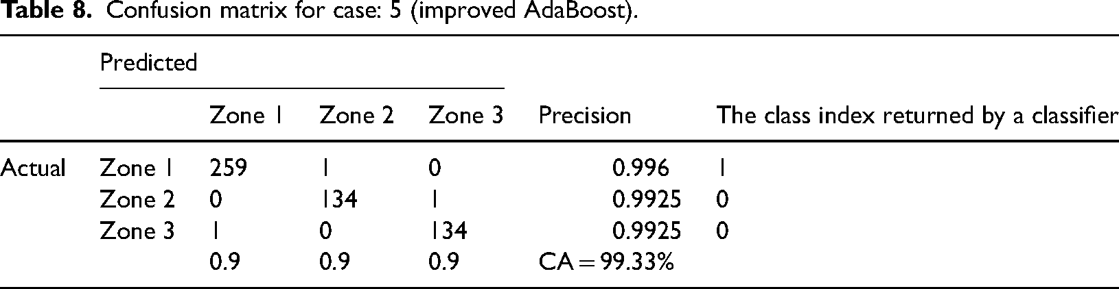
In this experiment, the fault signal data sets are acquired at the meters installed on Buses 24, and 22. In addition to this, the nonfault data sets are obtained at the various meters that are connected in the specified location. Here 530 data sets are gathered from all the meters and after applying TQWT the coefficients are fed into the AdaBoost classifier to classify the fault zone. Table 8 shows the confusion matrix for Case 5. According to Table 8, 259 of the 260 fault samples are classified as zone 1 in the confusion matrix, with a precision value of 0.99. The total efficiency of the observed categorization task is around 99.33%.

iii) Unbalanced distribution system with DG

Table 8.

Confusion matrix for case: 5 (improved AdaBoost).

	Predicted				Precision	The class index returned by a classifier
		Zone 1	Zone 2	Zone 3	Precision	The class index returned by a classifier
Actual	Zone 1	259	1	0	0.996	1
	Zone 2	0	134	1	0.9925	0
	Zone 3	1	0	134	0.9925	0
		0.9	0.9	0.9	CA = 99.33%

Practically most of the distribution networks are imbalanced after the integration of DG resources, storage units (ESD, and electrical vehicles (EV). In this work, the IEEE 33-bus standard test system is used to test the suggested technique (Dolatabadi et al., 2021). The block diagram of the IEEE 33 meshed distribution system with the DG placement is shown in Figure 14. Here DGs are connected at Buses 18, 22, 25, and 33. The DGs are linked by voltage source converters and regulated using the standard droop control approach. In this work, Buses 29 and 25, Buses 21 and 8, and Buses 22 and 12 are sewed together to form the radial bus system which is represented with a dotted line. In the IEEE 33-bus system, HIF is simulated between Buses 23 and 25. Here 530 data sets are captured. According to Table 9, it is observed that 259 fault data sets are identified and assigned to Zone 1 out of 260 fault data sets. This signifies that the occurrence of a fault is confined to Zone 1. The categorization problem has an overall efficiency of 99.33%.

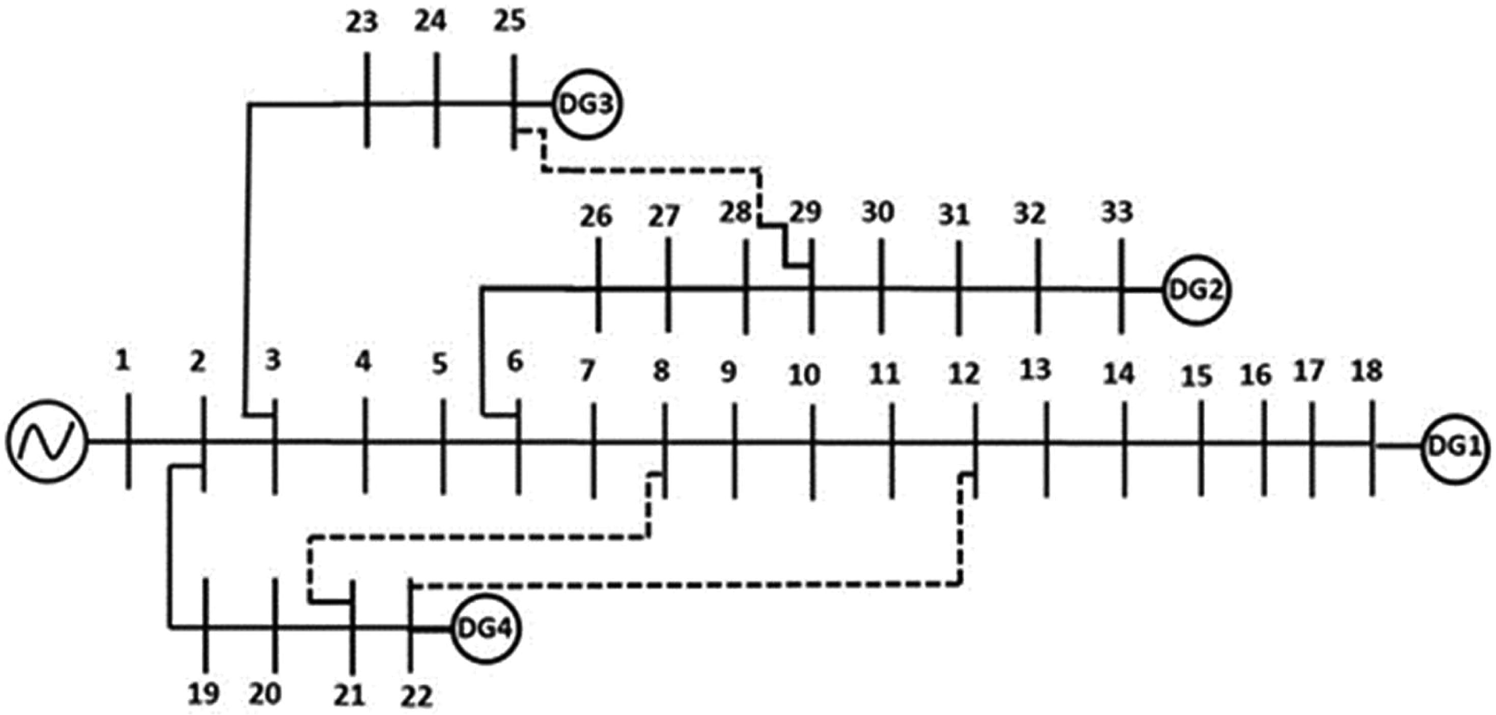
F. Case 6: Verification of the method in IEEE 123 unbalanced network

Figure 14.

Single line diagram of IEEE 33 distribution system.

Table 9.

Confusion matrix for case: 5 (improved AdaBoost classifier).

	Predicted				Precision	The class index returned by a classifier
		Zone 1	Zone 2	Zone 3	Precision	The class index returned by a classifier
Actual	Zone 1	259	1	0	0.996	1
	Zone 2	1	134	0	0.992	0
	Zone 3	1	0	134	0.992	0
					CA = 99.33%

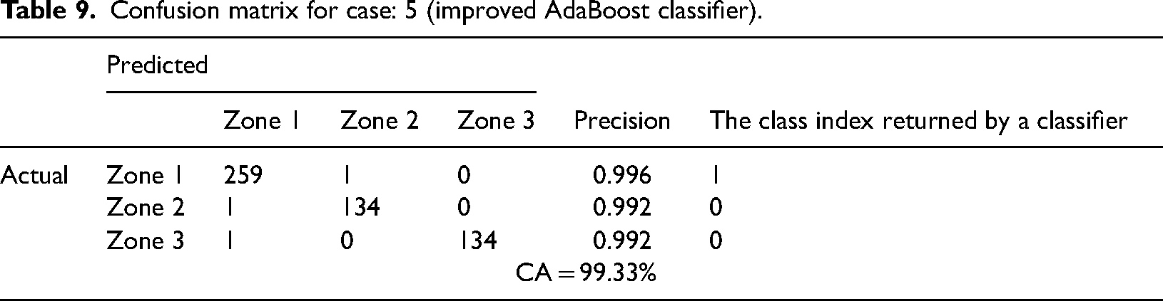
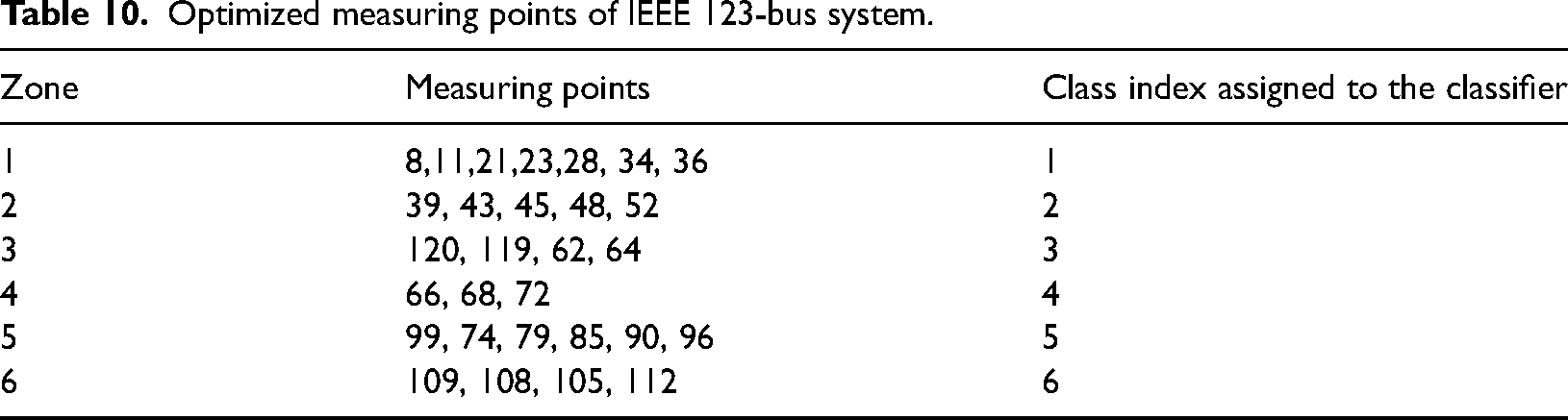
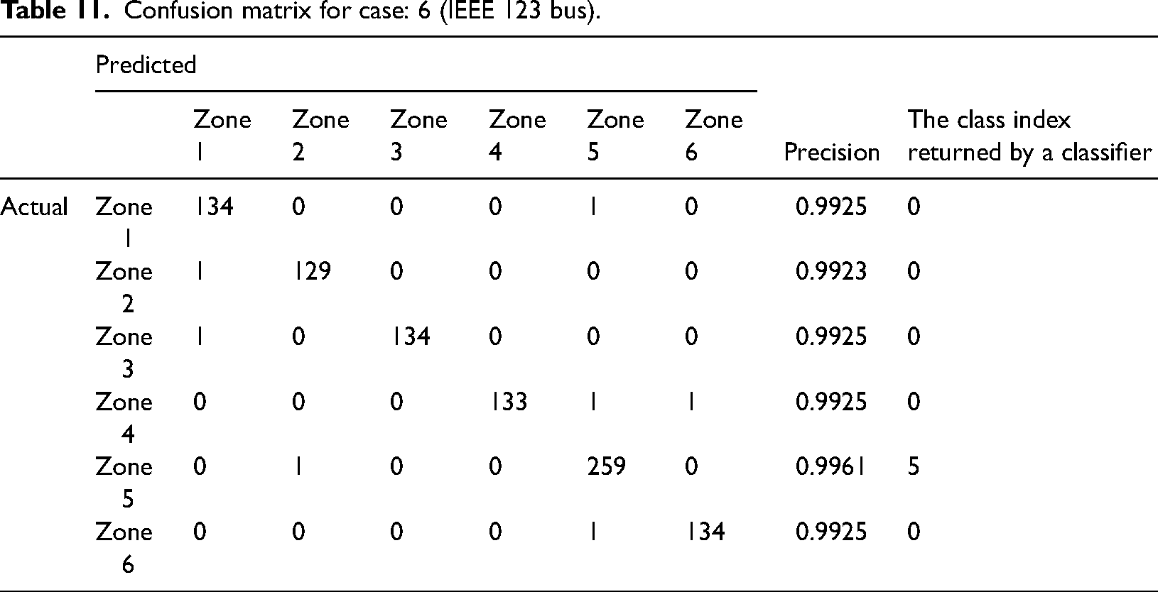
In this section, numerical simulations are performed in the modified IEEE 123-bus test case to demonstrate the proposed scheme. The single-line diagram of the IEEE 123-bus system is shown in Figure 15. Based on the Graph theory-based approach this network is divided into six zones which are shown in Figure 16. In Table 10 zones with specific buses are mentioned clearly. In this network, HIF has been created between Buses 85 and 86. According to Table 11, it is observed that 259 fault data sets are identified and assigned to Zone 5 out of 260 fault data sets. This signifies that the Zone 5 fault has occurred. The categorization problem has an overall efficiency of 99.46%.

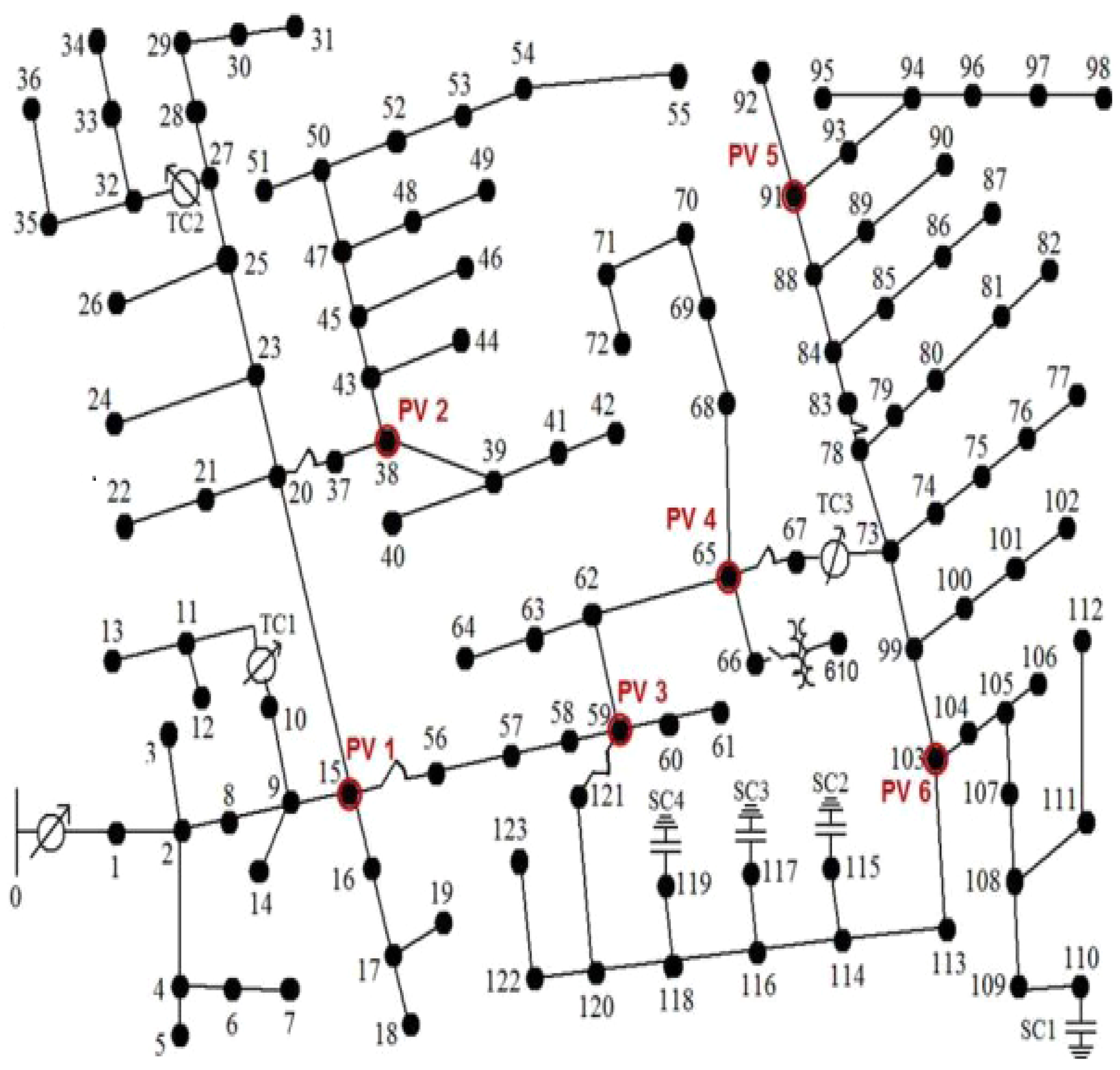
G. Case 7: Evaluation of the proposed method using RTDS

Figure 15.

IEEE 123 bus unbalanced distribution system.

Figure 16.

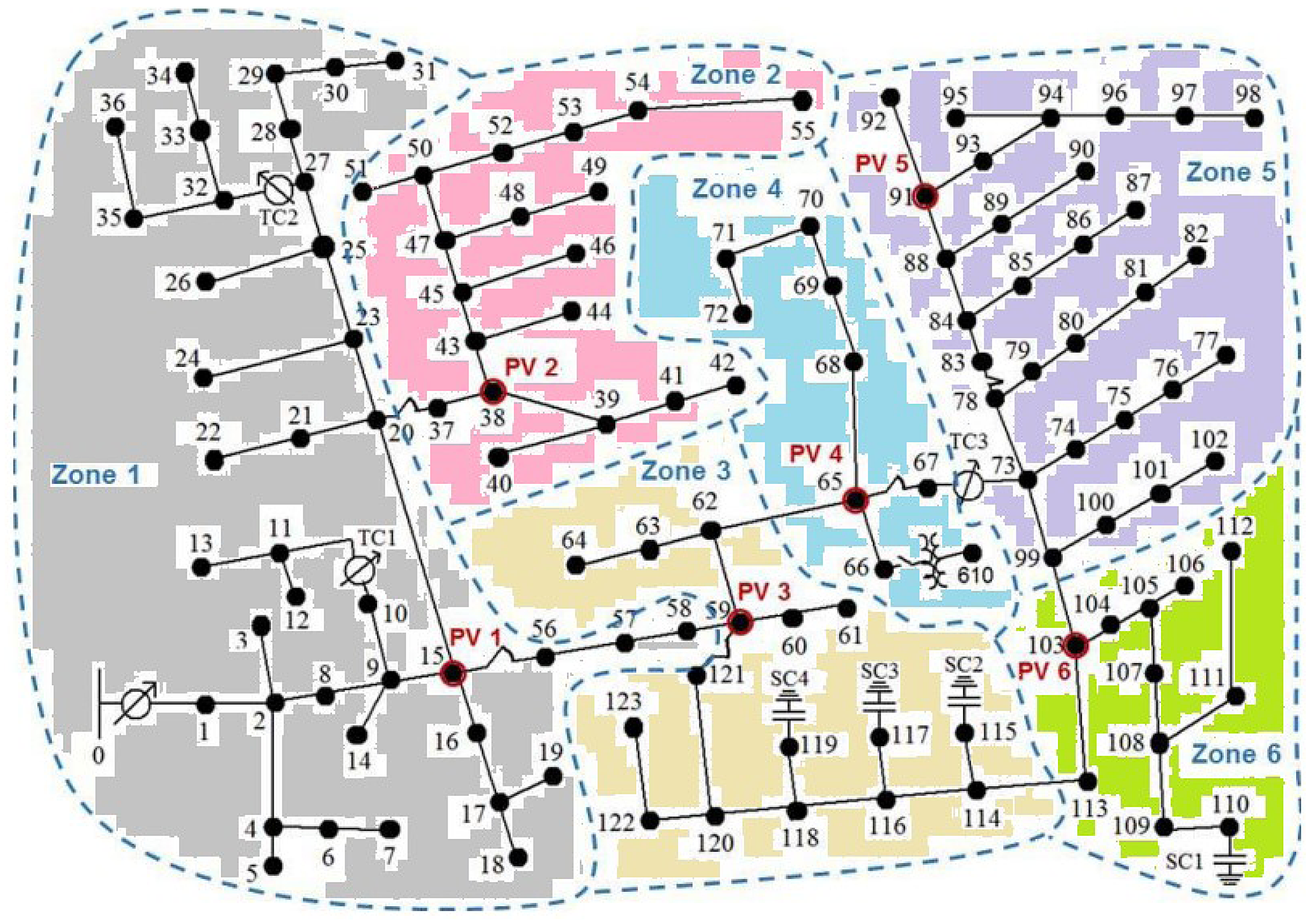
Zone division of IEEE 123 unbalanced distribution system.

Table 10.

Optimized measuring points of IEEE 123-bus system.

Zone	Measuring points	Class index assigned to the classifier
1	8,11,21,23,28, 34, 36	1
2	39, 43, 45, 48, 52	2
3	120, 119, 62, 64	3
4	66, 68, 72	4
5	99, 74, 79, 85, 90, 96	5
6	109, 108, 105, 112	6

Table 11.

Confusion matrix for case: 6 (IEEE 123 bus).

	Predicted							Precision	The class index returned by a classifier
		Zone 1	Zone 2	Zone 3	Zone 4	Zone 5	Zone 6	Precision	The class index returned by a classifier
Actual	Zone 1	134	0	0	0	1	0	0.9925	0
	Zone 2	1	129	0	0	0	0	0.9923	0
	Zone 3	1	0	134	0	0	0	0.9925	0
	Zone 4	0	0	0	133	1	1	0.9925	0
	Zone 5	0	1	0	0	259	0	0.9961	5
	Zone 6	0	0	0	0	1	134	0.9925	0

For the experimental verification of the proposed method in the hardware platform, the authors have fed the IEEE 33-bus distribution system in the RTDS system. The considered model is simulated in PSim and the simulation has been carried out by utilizing Opal-RT RTS OP5600 chassis with RT lab form of 11.X. Voltage signals consequently produced by Opal-RT real-time test system, have been sent to IO cards ML605 to gather the required information. The assessment of the proposed strategy for the location of HIF incorporates (i) the impact of sampling rates; (ii) the impact of random noise; and (iii) evaluation under DGs.

i) Influence of sampling rate

Sampling rates are very important for the measurement of voltage/current signals utilizing the HIF detection technique. The digitization of voltage and current signals uses sampling rates in such a way that the signature of the signal should be intact. To assess the impact of the sampling rate for detecting HIF, four different sampling frequencies are considered, that is, 4, 10, 51.2, and 89.6 kHz have been chosen. The proposed strategy precisely identifies HIF at all sampling frequencies. The proposed methodology can detect HIF accurately at all sampling frequencies. But here particular the industrial sampling frequency has been used, that is, 12.5 kHz for this work. The hardware model of the proposed scheme is shown in Figure 17.

ii) Fault in IEEE 33 radial distribution under noisy condition

Figure 17.

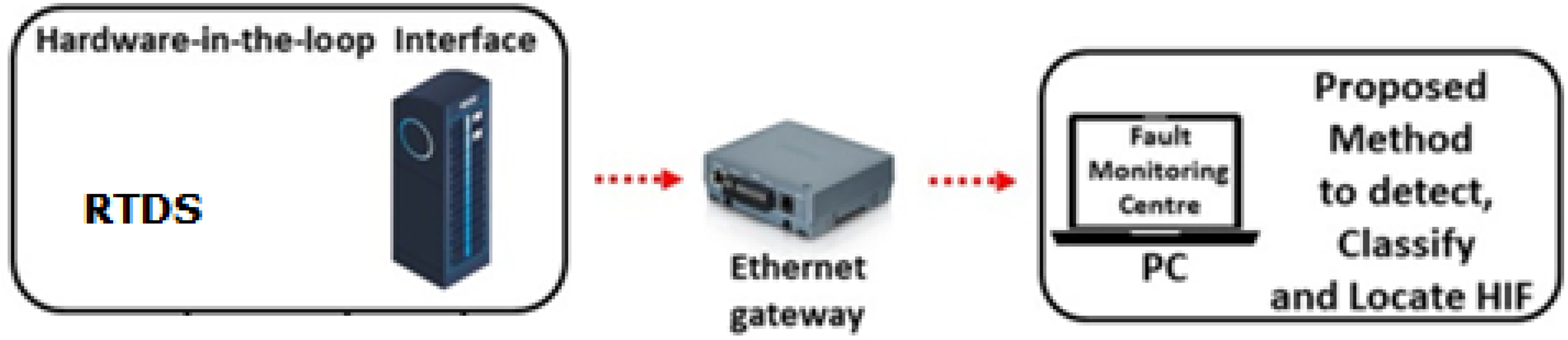
Hardware model of the proposed scheme.

The detection of the HIF zone has been subjected to a noisy environment in the hardware platform. Proper analysis of the noise impact is performed to evaluate the effectiveness of the projected approach. The signal-to-noise ratio (SNR) technically denotes noise, which is given by Equation (50).

{SNR}_{d b} = 20 \log_{10} (\frac{X_{signal}}{X_{noise}})

(50)

Here the problem occurred between Buses 5 and 16 in the presence of noise levels of 35, 25, and 10 dB. TQWT signal-processing technology is used to evaluate the fault signal and fault data sets are gathered at SMs positioned on Buses 14 and 17. Levels 4 and 5 detail coefficients derived from the fault signal. The nonfault data sets are obtained from the SMs located throughout the test system. The arc voltage at various noisy conditions is shown in Figure 18(a). In Figure 18(b), Kurtogram of noisy (10 dB) has been shown where up to 13th order harmonics are visible.

Figure 18.

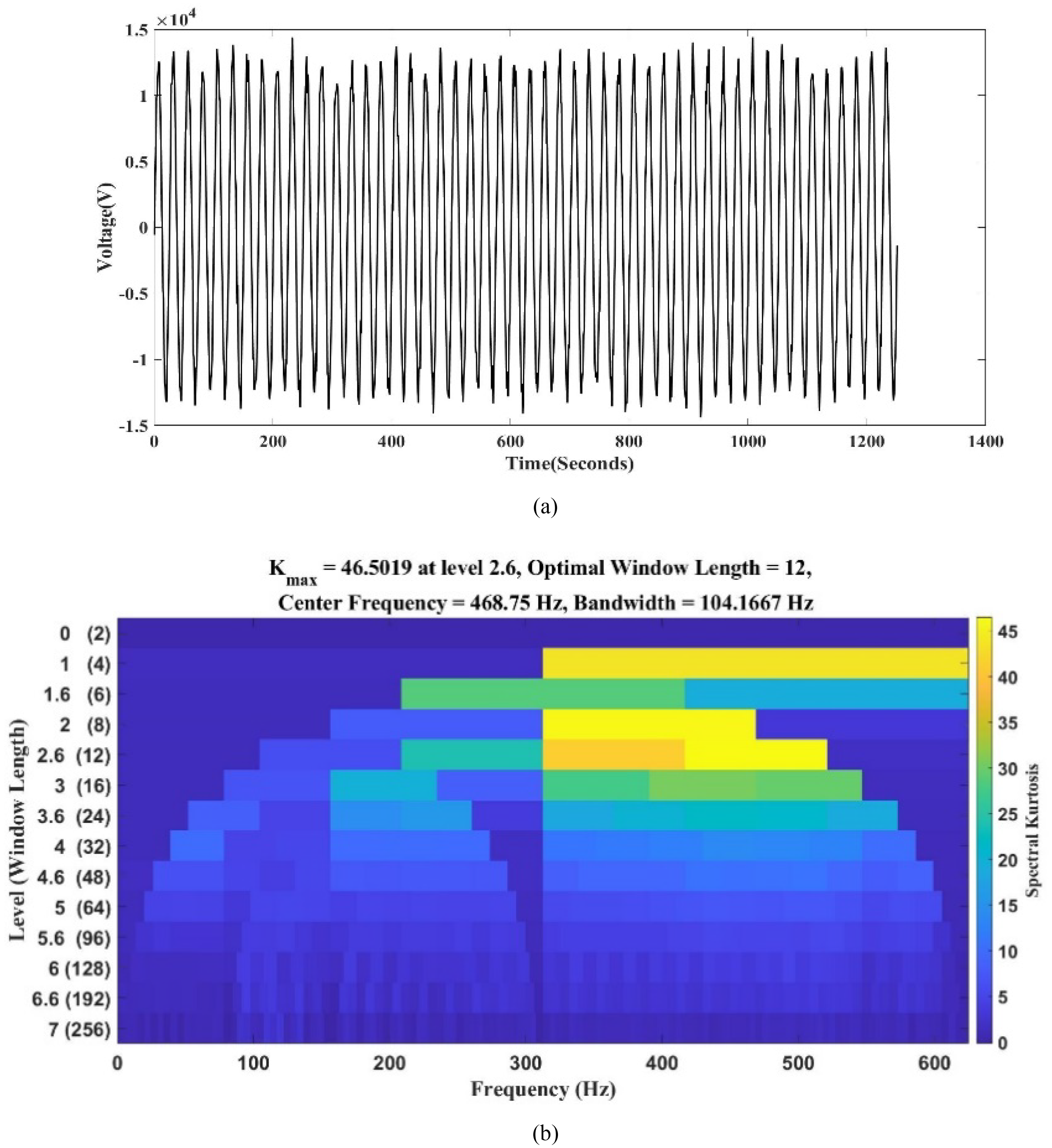
(a) Arc Voltage at various noisy conditions (25 dB and 10 dB), and (b) Arc Kourtogram of voltage at various noisy conditions (10 dB).

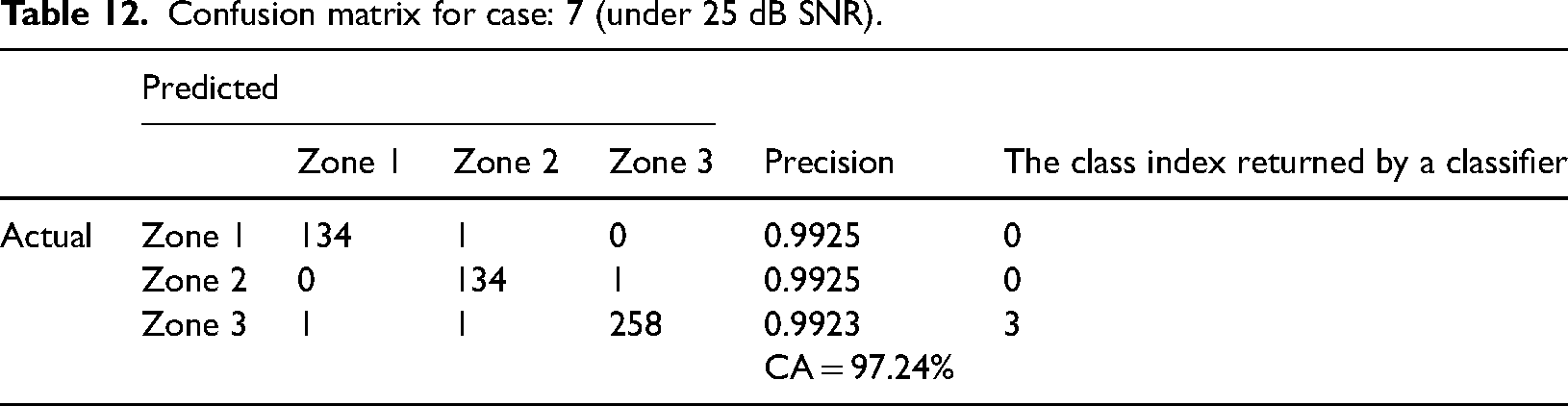
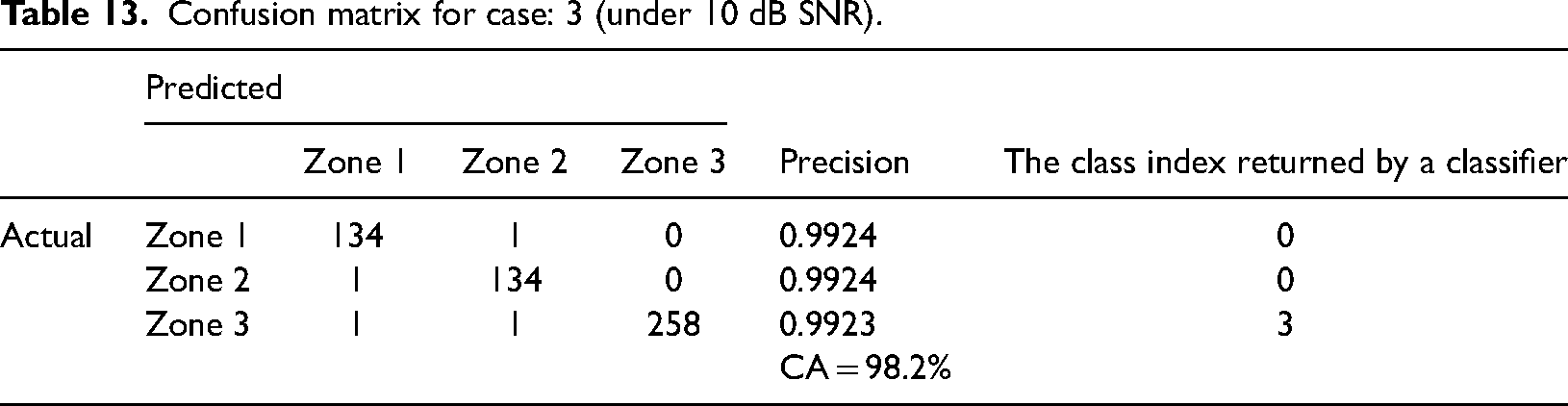
Here 260 fault signals are given to the classification task. In 25 dB SNR noisy condition, out of 260 fault signals, 250 signals are categorized as Zone 3 as its fault zone, with a classification accuracy of 99.24%. The confusion matrix of Case 7 under 25 dB SNR noisy condition is shown in Table 12. In 15 dB SNR noisy condition, out of 260 fault signals, 258 signals are categorized as Zone 3 as its fault zone with a classification accuracy of 99.23%. The confusion matrix of Case 3 under 25 dB SNR noisy condition is shown in Table 13.

iii) Performance of the proposed method in the presence of DG

Table 12.

Confusion matrix for case: 7 (under 25 dB SNR).

	Predicted				Precision	The class index returned by a classifier
		Zone 1	Zone 2	Zone 3	Precision	The class index returned by a classifier
Actual	Zone 1	134	1	0	0.9925	0
	Zone 2	0	134	1	0.9925	0
	Zone 3	1	1	258	0.9923	3
					CA = 97.24%

Table 13.

Confusion matrix for case: 3 (under 10 dB SNR).

	Predicted				Precision	The class index returned by a classifier
		Zone 1	Zone 2	Zone 3	Precision	The class index returned by a classifier
Actual	Zone 1	134	1	0	0.9924	0
	Zone 2	1	134	0	0.9924	0
	Zone 3	1	1	258	0.9923	3
					CA = 98.2%

To meet the recent trend, grid-connected DG has been considered in the IEEE 33-bus system and verified this method in a hardware platform using RTDS. In this case, a wind farm with wind-driven DFIG including an AC/DC/AC insulated-gate bipolar transistor (IGBT)-based pulse width modulation (PWM) converter has been considered. The value of HIF at various inception angles with varying fault resistance is considered at Nodes 27, 10, and 3 in association with the DGs and measured data collected from the optimal location of the measuring points of the IEEE 33-bus system. In Table 14, it is shown that fault occurs at Zone 2 as external HIF has been created at this zone, and here the success rate is 99.25%.

Table 14.

Confusion matrix after considering DGs in IEEE 33-bus system.

N = 400	Predicted				%
N = 400		Zone 1	Zone 2	Zone 3	%
Actual	Zone 1	134	1	0
	Zone 2	1	259	0
	Zone 3	1	0	124
					99.25

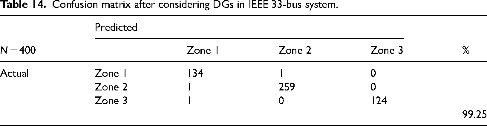
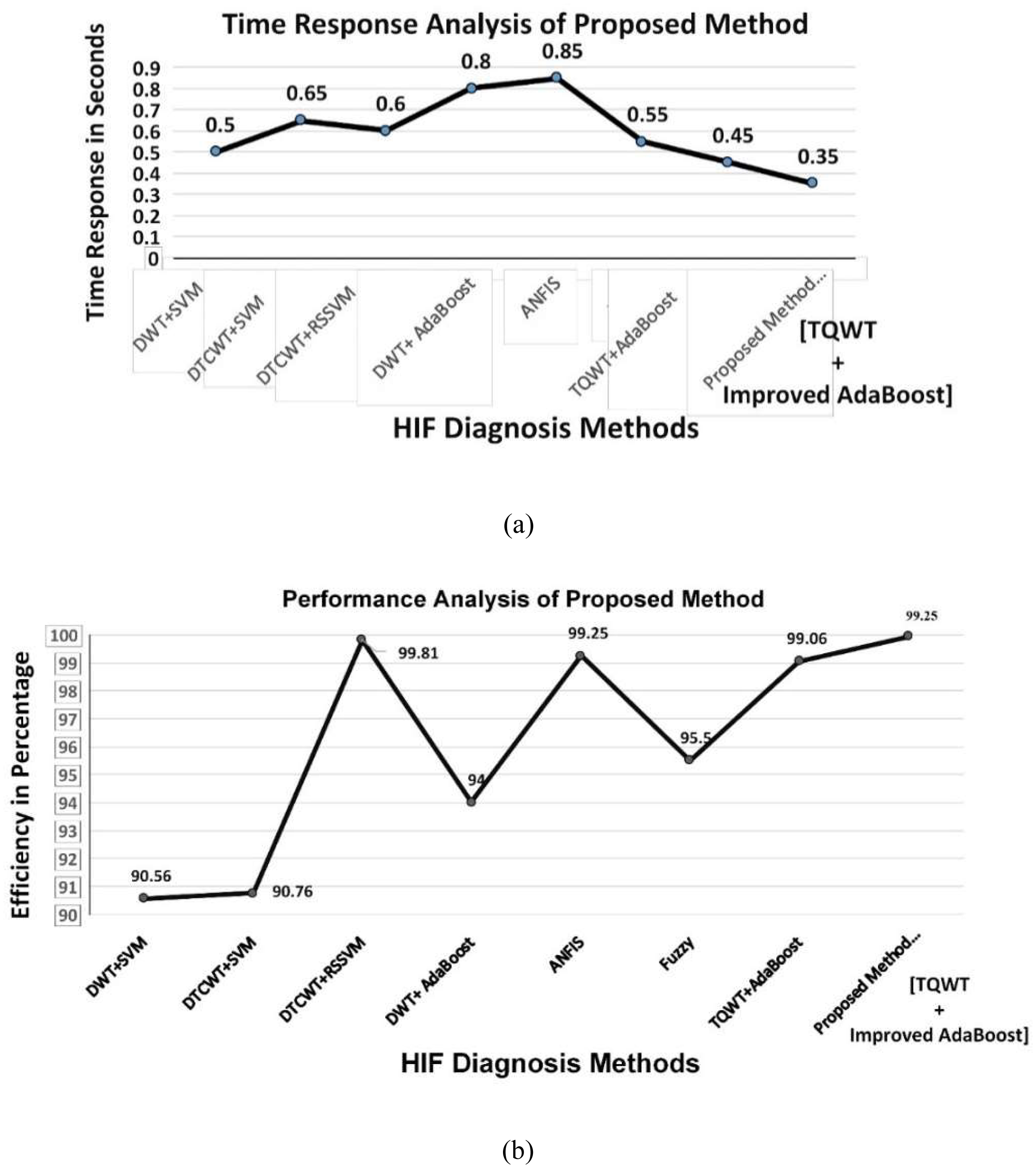
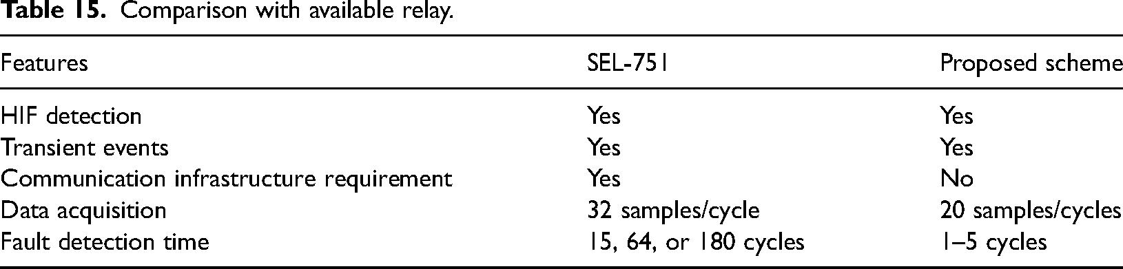
Figure 19(a) describes that the improved AdaBoost needs the lowest time as compared with the other existing methods and Figure 19(b) depicts the pictorial view of the performance analysis of the proposed method. Table 15 shows the comparison of the proposed method with SEL 751.

Figure 19.

Part figures (a) and (b) performance analysis of improved AdaBoost.

Table 15.

Comparison with available relay.

Features	SEL-751	Proposed scheme
HIF detection	Yes	Yes
Transient events	Yes	Yes
Communication infrastructure requirement	Yes	No
Data acquisition	32 samples/cycle	20 samples/cycles
Fault detection time	15, 64, or 180 cycles	1–5 cycles

Analytical summary of the proposed work

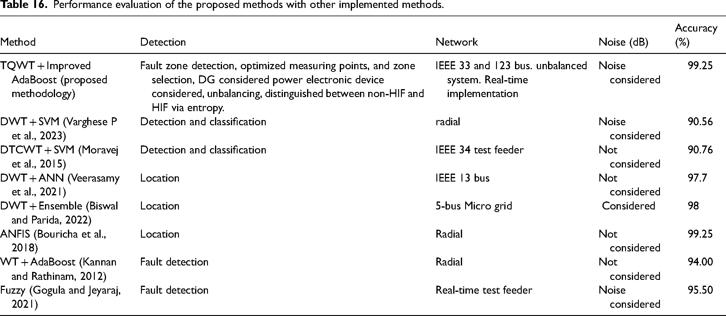
The effectiveness of the projected TQWT-based voltage/current-based HIF fault-finding methodology has been accomplished in the manuscript. This method is first verified for HIF faults in the IEEE 33 bus distribution system and then the IEEE 123 unbalanced distribution system. The presented method is verified under different conditions to justify its performance. The TV of the projected approach doesn’t alter and remains fixed for all extensive test cases as it normalized based on Equation (21). This article proposes a fault zone identification technique for balanced and unbalanced distribution systems utilizing voltage signals. The suggested approach places measurement devices at appropriate locations using the Jellyfish Search optimization technique to create a new zone protection strategy. The suggested approach is used on IEEE 33-bus balanced and IEEE 123-bus unbalanced distribution systems. This strategy works with distributed generation, power electronics devices, and noise. The outcome analysis shows the methodology’s overall 99.06% efficiency. The comparative analysis of the proposed approach has been shown in Table 16. This study concludes that the proposed system ensures measurement equipment in each Zone. The proposed technology is cost-effective compared to conventional zone protection methods. This strategy reduces memory.

Table 16.

Performance evaluation of the proposed methods with other implemented methods.

Method	Detection	Network	Noise (dB)	Accuracy (%)
TQWT + Improved AdaBoost (proposed methodology)	Fault zone detection, optimized measuring points, and zone selection, DG considered power electronic device considered, unbalancing, distinguished between non-HIF and HIF via entropy.	IEEE 33 and 123 bus. unbalanced system. Real-time implementation	Noise considered	99.25
DWT + SVM (Varghese P et al., 2023)	Detection and classification	radial	Noise considered	90.56
DTCWT + SVM (Moravej et al., 2015)	Detection and classification	IEEE 34 test feeder	Not considered	90.76
DWT + ANN (Veerasamy et al., 2021)	Location	IEEE 13 bus	Not considered	97.7
DWT + Ensemble (Biswal and Parida, 2022)	Location	5-bus Micro grid	Considered	98
ANFIS (Bouricha et al., 2018)	Location	Radial	Not considered	99.25
WT + AdaBoost (Kannan and Rathinam, 2012)	Fault detection	Radial	Not considered	94.00
Fuzzy (Gogula and Jeyaraj, 2021)	Fault detection	Real-time test feeder	Noise considered	95.50

Conclusions

In this work, a unique graph theory and improved AdaBoost -based approach for detection, classification, and zone identification of HIFs in distribution systems are proposed. In TQWT, the QF can be adjusted based on the oscillatory nature of the signal. Furthermore, this transform is based on expansion factors and is achieved using an oversampled filter bank with perfect reconstruction using real-valued sampling factors. An entropy measurement-based approach is applied to extract specific features from the decomposed signal. Entropy measurements provided decision rules for recognizing and classifying high-impedance defects. An improved AdaBoost machine learning classifier technique is applied to detect the faulted zones. Choosing a proper decomposition level based on the K value and the use of an improved AdaBoost makes the mythology faster than the other existing method which has been proved by Figure 19. The proposed methodology can be used for the commercial relay feeder protection system as it is verified in the hardware model with high efficiency. Despite alterations in the configuration of the power system distribution network, the proposed technique pinpoints faulty zones. The proposed technique collects more data/information from optimally located measuring devices, reducing the cost of the proposed method. A sampling frequency selection approach improves the accuracy of this technique. This methodology has been tested for both balanced and unbalanced networks under noisy conditions. The proposed approach is successful under both high-noise and low-noise conditions, demonstrating the robustness of the algorithm. The authors of this paper have shown that choosing an appropriate number of decomposition levels minimizes the computational complexity and speeds up the method. The proposed approach is verified using the real-time platform by developing the IEEE 33-bus test system, the unbalanced modified IEEE 33-bus test system, and the IEEE 123-bus test system. It is also used in real-time systems. This proposed technique shows excellent accuracy in all case studies. Therefore, this technique can suitably be applied in a real-time power system distribution network to identify, classify, and pinpoint high-impedance problems.

Footnotes

Acknowledgments

The authors are grateful for the support of the Researchers Supporting Project (number RSP2024R258), King Saud University, Riyadh, Saudi Arabia.

Declaration of conflicting interests

The authors declared no potential conflicts of interest with respect to the research, authorship, and/or publication of this article.

Ethical approval

This article does not contain any studies with human or animal participants.

ORCID iDs

Daniel Eutyche Mbadjoun Wapet

Mohamed Metwally Mahmoud

Data Availability Statement

Data are available on request from the authors.

References

Biswal

Parida

(2022) A novel high impedance fault detection in the micro-grid system by the summation of accumulated difference of residual voltage method and fault event classification using discrete wavelet transforms and a decision tree approach. Electric Power Systems Research 209: 108042–108059. DOI: https://doi.org/10.1016/j.epsr.2022.108042.

Bouricha

Bouthiba

Boukhari

, et al. (2018) High Impedance Faults Location in the Distribution Networks Using Adaptive Neuro-Fuzzy Inference System. In: Proceedings of 2018 3rd International Conference on Electrical Sciences and Technologies in Maghreb, CISTEM 2018.

CAO

Miao

Q-G

Liu

J-C

, et al. (2013) Advance and prospects of AdaBoost algorithm. Acta Automatica Sinica 39(6): 745–58.

Chou

Truong

(2021) A novel metaheuristic optimizer inspired by behavior of jellyfish in ocean. Applied Mathematics and Computation 389: 125535–125582. DOI: https://doi.org/10.1016/j.amc.2020.125535.

Ding

Zhou

Yin

(2019) Fault detection and diagnosis of a Wheelset-bearing system using a multi-Q-factor and multi-level tunable Q-factor wavelet transform. Measurement: Journal of the International Measurement Confederation 143: 112–24.

Dolatabadi

Ghorbanian

Siano

, et al. (2021) An enhanced IEEE 33 bus benchmark test system for distribution system studies. IEEE Transactions on Power Systems 36(3): 2565–72.

Dubey

Jena

(2020) Impedance angle-based differential protection scheme for microgrid feeders. IEEE Systems Journal 15(3): 3291–3300.

Elmetwaly

Younis

Abdelsalam

, et al. (2023) Modeling, simulation, and experimental validation of a novel MPPT for hybrid renewable sources integrated with UPQC: an application of jellyfish search optimizer. Sustainability (Switzerland) 15(6): 5209–5239.

Every

Dorrell

(2017) Leveraging smart meter data for economic optimization of residential photovoltaics under existing tariff structures and incentive schemes. Applied Energy 201: 158–73.

10.

Gautam

Brahma

(2013) Detection of high impedance fault in power distribution systems using mathematical morphology. IEEE Transactions on Power Systems 28(2): 1226–34.

11.

Gogula

Jeyaraj

(2021) A Wavelet-Fuzzy Combined Approach for Detection on High Impedance Faults in Distribution Systems. In: 3rd IEEE international virtual conference on innovations in power and advanced computing technologies, i-PACT 2021. 27–29 November 2021, IEEE, Kuala Lumpur, Malaysia. DOI: https://doi.org/10.1109/i-PACT52855.2021.9697042.

12.

Huang

Z-J

Wang

J-M

, et al. (2021) High impedance fault detection in overhead distribution feeders using a DSP-based feeder terminal unit. IEEE Transactions on Industry Applications 57(1): 179–86.

13.

Hamatwi

Imoru

Kanime

, et al. (2023) Comparative analysis of high impedance fault detection techniques on distribution networks. IEEE Access 11: 25817–34.

14.

Ibrahim

Alkuhayli

Beroual

, et al. (2023) Enhancing the functionality of a grid-connected photovoltaic system in a distant Egyptian region using an optimized dynamic voltage restorer : application of artificial rabbits optimization. Sensors (Switzerland) 23(16): 7146.

15.

Ibrahim

Mahmoud

HAl Thaiban

, et al. (2023) Operation of grid-connected PV system with ANN-based MPPT and an optimized LCL filter using GRG algorithm for enhanced power quality. IEEE Access (September): 1.

16.

Izadi

Mohsenian-Rad

(2022) A synchronized Lissajous-based method to detect and classify events in synchro-waveform measurements in power distribution networks. IEEE Transactions on Smart Grid 13(3): 2170–84.

17.

Jalil

Samet

Ghanbari

, et al. (2021) An enhanced Cassie-Mayr-based approach for DC series arc modeling in PV systems. IEEE Transactions on Instrumentation and Measurement 70: 1–10. DOI: https://doi.org/10.1109/TIM.2021.3124832.

18.

Joga

SRK

Sinha

Maharana

(2021a) Genetic algorithm and graph theory approach to select protection zone in distribution system. Lecture Notes in Electrical Engineering 688: 165–74. doi:https://doi.org/10.1007/978-981-15-7241-8_13.

19.

Joga

SRK

Sinha

Maharana

(2021b) Performance study of various machine learning classifiers for arc fault detection in AC microgrid. IOP Conference Series: Materials Science and Engineering 1131(1): 012012.

20.

Kannan

Rathinam

(2012) High impedance fault classification using wavelet transform and artificial neural network. In: Proceedings of 4th international conference on computational intelligence and communication networks, 3–5 November 2012, Mathura, IEEE, 2012, pp. 831–37. DOI:https://doi.org/10.1109/CICN.2012.122.

21.

Ledesma

JJG

De Araujo

RPDARP

(2021) A method for the approximate location of high impedance faults using neural networks. IEEE Latin America Transactions 19(3): 351–58.

22.

Liu

, et al. (2022) An FTU-based method for locating single-phase high-impedance faults using transient zero-sequence admittance in resonant grounding systems. IEEE Transactions on Power Delivery 37(2): 913–22.

23.

Mahmoud

Atia

Esmail

, et al. (2023) Application of whale optimization algorithm based FOPI controllers for STATCOM and UPQC to mitigate harmonics and voltage instability in modern distribution power grids. Axioms 12(5): 420–446. DOI: https://doi.org/10.3390/axioms12050420.

24.

Mahmoud

Esmail

Atia

, et al. (2022) Voltage quality enhancement of low-voltage smart distribution system using robust and optimized DVR controllers : application of the Harris Hawks algorithm. International Transactions on Electrical Energy Systems 2022: 18.

25.

Mahmoud

Ratib

Aly

, et al. (2022) Wind-driven permanent magnet synchronous generators connected to a power grid: existing perspective and future aspects. Wind Engineering 46(1): 189–99.

26.

Marcos

Fernando E. Postigo

Mateo

Carlos

Gomez

Tomás

, et al. (2017) “A review of power distribution test feeders in the United States and the need for synthetic representative networks.” Energies 10(11).

27.

Meera

Hemamalini

(2017) Optimal siting of distributed generators in a distribution network using artificial immune system. International Journal of Electrical and Computer Engineering 7(2): 641–49.

28.

Metwally Mahmoud

(2023) Improved current control loops in wind side converter with the support of wild horse optimizer for enhancing the dynamic performance of PMSG-based wind generation system. International Journal of Modelling and Simulation 43(6): 952–66.

29.

Moravej

Mortazavi

Shahrtash

(2015) DT-CWT based event feature extraction for high impedance faults detection in distribution system. International Transactions on Electrical Energy Systems 25(12): 3288–3303.

30.

Nir

Sela

Beck

, et al. (2020) Machine-learning iterative calculation of entropy for physical systems. Proceedings of the National Academy of Sciences of the United States of America 117(48): 30234–40.

31.

Oliveira

RAd

Bollen

MHJ

(2023) Deep learning for power quality. Electric Power Systems Research 214: 108887–108899. DOI: https://doi.org/10.1016/j.epsr.2022.108887.

32.

Ozansoy

(2020) Performance analysis of skewness methods for asymmetry detection in high impedance faults. IEEE Transactions on Power Systems 35(6): 4952–55.

33.

Reddy

GRS

Rao

(2016) Extraction of fundamental component in power quality application using tunable-Q wavelet transform. International Journal of Signal Processing, Image Processing and Pattern Recognition 9(8): 355–80.

34.

Shaowen

Yong

(2015) A kind of improved AdaBoost algorithm. In: Proceedings of 7th international conference on intelligent computation technology and automation, 25 -26 October 2014, Changsha, China, IEEE, 16–18. DOI:https://doi.org/10.1109/ICICTA.2014.11.

35.

Sharma

Samantaray

Bhende

(2022) VMD-enabled current-based fast fault detection scheme for DC microgrid. IEEE Systems Journal 16(1): 933–44.

36.

Sheng

Liu

Jia

, et al. (2024) An improved high-impedance fault identification scheme for distribution networks based on kernel extreme learning machine. International Journal of Electrical Power and Energy Systems 155: 109543–109553. DOI: https://doi.org/10.1016/j.ijepes.2023.109543.

37.

Shi

Huang

Shen

, et al. (2019) Dual-guidance-based optimal resonant frequency band selection and multiple ridge path identification for bearing fault diagnosis under time-varying speeds. IEEE Access 7: 144995–12.

38.

Silva

Costa

Santana

, et al. (2020) Evolving neuro-fuzzy network for real-time high impedance fault detection and classification. Neural Computing and Applications 32(12): 7597–7610.

39.

Teimourzadeh

Member

(2021) High impedance single-phase faults diagnosis in transmission lines via deep reinforcement learning of transfer functions. IEEE Access 9: 15796–809.

40.

Thirumala

Prasad

Jain

, et al. (2018) Tunable-Q wavelet transform and dual multiclass SVM for online automatic detection of power quality disturbances. IEEE Transactions on Smart Grid 9(4): 3018–28.

41.

Liu

(2017) AdaBoost typical algorithm and its application research. In: MATEC Web of Conferences. 5 December 2017, China, EDP Sciences, pp. 222–228. DOI: https://doi.org/10.1051/matecconf/201713900222.

42.

Valenza

Citi

Scilingo

, et al. (2013) Point-process nonlinear models with Laguerre and Volterra expansions: instantaneous assessment of heartbeat dynamics. IEEE Transactions on Signal Processing 61(11): 2914–26.

43.

Varghese P

Subathra

MSP

Thomas George

, et al. (2023) Application of signal processing techniques and intelligent classifiers for high-impedance fault detection in ensuring the reliable operation of power distribution systems. Frontiers in Energy Research 11: 1114230–1114264.

44.

Veerasamy

Wahab

NIA

Othman

, et al. (2021) LSTM recurrent neural network classifier for high impedance fault detection in solar PV integrated power system. IEEE Access 9: 32672–87.

45.

Wang

Cui

(2022) Nonlinear modeling analysis and arc high-impedance faults detection in active distribution networks with neutral grounding via Petersen coil. IEEE Transactions on Smart Grid 13(3): 1888–98.

46.

Xiao

Guo

Chen

(2022) High-impedance fault detection method based on one-dimensional variational prototyping-encoder for distribution networks. IEEE Systems Journal 16(1): 966–76.

47.

Yang

Guo

Zhang

, et al. (2022) Classification of multiple power quality disturbances by tunable-Q wavelet transform with parameter selection. Energies 15(9.

48.

Yuan

Sheng

Zhuang

, et al. (2024) A novel fault diagnosis method for second-order bandpass filter circuit based on TQWT-CNN. PLoS ONE 19(2)): 1–19. DOI: https://doi.org/10.1371/journal.pone.0291660.

49.

Zhang

, et al. (2022) Feature enhancement based on regular sparse model for planetary gearbox fault diagnosis. IEEE Transactions on Instrumentation and Measurement 71: 1–16.

50.

Zhang

, et al. (2019) Research and application of AdaBoost algorithm based on SVM. In: Proceedings of 2019 IEEE 8th Joint International Information Technology and Artificial Intelligence Conference, 24–26 May 2019, IEEE, Chongqing, China, pp. 662–66. DOI:https://doi.org/10.1109/ITAIC.2019.8785556. 662–66.

51.

Zhao

(2017) Fault diagnosis of wind turbine bearing based on variational mode decomposition and Teager energy operator. IET Renewable Power Generation 11(4): 453–60.

Applications of tunable-Q factor wavelet transform and AdaBoost classier for identification of high impedance faults: Towards the reliability of electrical distribution systems

Abstract

Keywords

Introduction

Major contributions

The problematization of the issue

Simulation of the HIF

Method for the decomposition of signals based on the TQWT

Calculation of entropy

The determination of the best possible number of levels of decomposition

Selection of decomposition level and mother wavelet

Enhanced AdaBoost machine learning classifier

Optimal location selection of smart meters (SMs) using Jellyfish Optimizer (JFO)

JFO technique

Ocean current

Swarming occurrence of Jellyfish

Time control mechanism

The beginning stages of the inhabitants of jellies

Boundary condition

Graph Search Technique for Partitioning Off Protective Zones

Results and discussions

Analytical summary of the proposed work

Conclusions

Footnotes

Acknowledgments

Declaration of conflicting interests

Ethical approval

ORCID iDs

Data Availability Statement

References