Sage Journals: Discover world-class research

Abstract

Palestine lacks sufficient conventional energy sources that meet the daily needs of the Palestinian people, and consequently, it heavily relies on neighboring countries for its supply with energy compensations. Wind energy is recognized as an abundant, effective, and eco-friendly power source, but it poses several challenges in harnessing due to the inherent variability of wind characteristics. The main objective of this research study is to delve into the wind energy landscape in Palestine, and to offer some insights into the feasibility of wind speed forecasting for implementing sustainable energy solutions, with a special focus on ARIMA; a widely used statistical method for time series forecasting. It specifically explores the potential of using ARIMA models to forecast wind speed using a data captured from a meteorological station located in east Jerusalem, Palestine for a duration of 2 years—January 1, 2021 to December 31, 2022. To find the optimal values of ARIMA parameters (p, d, q) for the considered study site, a set of experiments were conducted and the model's forecasting accuracy was evaluated using three metrics: RMSE, MAE, and the coefficient of determination (R²). The results have shown that ARIMA (21,2) emerges as the most accurate structure with an input period that demonstrates superior estimation with minimal RMSE (1.74), minimal MAE (1.58) and higher R² (0.76) values. This means that the optimal estimation is achieved when an autoregressive process is based on the previous two lagged observations and the moving average process incorporates the dependency between the observation and the residual error from a second-order moving average applied to the lagged observations. These findings give valuable insights into the feasibility and precision of wind speed forecasting models for sustainable energy solutions, and emphasize the potential for harnessing wind energy in the region as clarified by ARIMA forecasting accuracy.

Keywords

Wind speed time series forecasting performance Arima RMSE MAE R-squared

Introduction

In the current era of the information age, the investment in renewable energy sources is attracting a global attention worldwide. Many countries are now investing huge budgets in renewable energy projects to meet their current and future energy needs (Elsaraiti and Merabet, 2021). The sun and wind energies are among the most important sources of energy sustainability in Palestine, where solar energy has received an in-depth study, but wind energy lacks studies at the national level, although it is one of the solutions to generate electricity, as it provides a clean and practical solution to generate energy from wind using small turbines similar to home solar projects (Hanifi et al., 2020). Since the wind speed is the main factor on which the amount of energy production depends, and there are not enough monitoring stations in terms of the highest construction and operational costs, the researchers are currently working toward the development of digital models that deeply analyze and predict the highly variable wind speed values at a specific study site for one region and circulate them to other areas (Chodakowska et al., 2023). Since the wind chaotic nature is large and considers a main challenge for producing energy. However, predicting wind speed accurately at a specific site must be given special attention when considering projects related to the installation of wind farms. Thus, before the development and installation of wind power applications at a site; the main challenge that requires special attention throughout the feasibility study is the wind speed profile at that site (Chen et al., 2022). In this regard, an accurate and deep analysis of wind profiles must be carried out to achieve higher prediction accuracy of wind energy at a meteorological station to get the optimal benefits out of the wind (Shang et al., 2022).

To compensate for their energy demands, the Palestinian people depend on neighboring countries. They lack their own sustainability in energy due to several challenges such as the bad political situations they live in, the economic issues induced by lockout and limited income, and other environmental and social issues (Alsamamra et al., 2022). For this reason, most areas of Palestine suffer from a severe shortage of energy supplies throughout the year, without any radical solutions appearing on the horizon (Juaidi et al., 2022b). Currently, the Palestinian Authority considers renewable energy sources as one of the top governmental priorities in its sustainable development goals (SDGs) plan for the coming years. It encourages and supports all development projects targeting this sustainable goal.

The geographical nature of Palestine helps to install wind turbines in some areas with good wind speed characteristics for generating electricity (Salah et al., 2022). The presented study is an important work since studies in exploring long-term wind speed profiles in east Jerusalem to predict wind are very limited. Although there are similar contributions conducted worldwide, the research community emphasized that the nature and characteristics of wind speed differ from location to location (site-dependent), and an optimal solution for one location is not necessary to be valid for others. Due to the lack of similar contributions in Palestine, this study's output will be used as a reference point for those who are planning to invest in wind energy projects in the region.

Palestine suffers from the scarcity of traditional energy sources, higher energy consumption prices, as well as the control of the occupation authority over the quantities that feed the Palestinian lands. As a result of this, the Palestinians always seek to rely more on alternative energy sources, as this approach comes in line with the growing global trends to exploit alternative energy sources. In this regard, the Palestinian Authority is continuously supporting all individuals and any collective initiative that works to produce electric energy from alternative sources (Ibrik, 2019). This was also represented in the Palestinian government enacting regulatory legislation that encourages investors to invest in renewable energy and regulates the relationship between the parties involved in any investment (PCBS, 2024). Also, the Ministry of Higher Education (MOHE) has worked to encourage the national universities to develop academic programs in renewable energy and support researchers in this field, recognizing the importance of the energy sector in general and an alternative energy in particular, because they believe that this sector contributes to achieving the independence of the energy sector which is one of the main factors in the independence of countries and sustainable development. Also, they believe that any sustainable energy project will create new job opportunities in society, since this sector opens many opportunities, and it is considered as one of the highest demanded professionals in the world (Abdallah and Camur, 2022).

Compared to other nearby countries, the energy sector in Palestine has special considerations due to several reasons: unstable political and economic conditions, a scarcity of natural resources, high population density, fully dependent on nearby countries and difficult financial problems (Hamed et al., 2012). Due to its weak economy, Palestine desperately needs all kinds of energy, the Palestinian government has recently adopted the renewable energy polices and implemented many projects aimed to increase the investment in the renewable energy sector (Juaidi et al., 2022a). Globally, in the next 30 years, the consumption of renewable energy will keep growing by a factor of 147% (Sun and Jin, 2022). However, investment projects in sustainable and clean energy have attracted global attention; for every 1 USD spent on fossil fuels, there is 1.7 USD is spent on clean energy compared to a 1:1 ratio 5 years ago (Li et al., 2023a). Compared to all sources of renewable energy, in 2021 wind-based energy increased by an amount of up to 17%, which was 45% higher growth compared to the year 2020, and it was the highest among all renewable energy technologies (GWEC, 2021). In their report, the Global Wind Energy Council (GWEC) stated that the international generated electricity based on wind power systems has an increase of 94 GW between the years 2021 and 2022 (GWEC, 2022). However, a precise knowledge of wind speed conditions at a wind farm plays a crucial role to the success of a project during assessments and operational phases. Furthermore, the increase of grid-connected wind power technology and the nonstationary of wind speed, the stability of the power system is a challenge (Kitaneh et al., 2012). Therefore, designing accurate wind speed forecasting models will help in building efficient wind power systems to get the best utilization out of this nature energy source by minimizing the side effects of wind uncertainties on the stability of these systems (Kosanoglu, 2022).

The remaining parts of the article are structured as follows. A review of the related work is presented in the second section. The technical description of the ARIMA model and its components are discussed in the third section. The fourth section presents the dataset and discusses the research methodology. The fifth section overviews the common performance metrics used to evaluate the proposed model. The results and their discussions are presented in the sixth section. The last section summarizes the main findings and provides further research lines.

Related work

Internationally, the significance in contributing intraday marketplaces is expanding as the amount of renewable irregular energy production expands. Being reasonable on the network closer to distribution time aids both power systems and market participants by shrinking the need for related costs and reserves. Additionally, the intraday marketplace is a vital instrument for market contributors to coordinate unforeseen shifts in energy consumption and outages (Shoaib et al., 2019). Wind speed has strong intermittency and randomness, and the continuous growth of the scale of the wind power systems might lead to a frequent destruction of the stability of the power system and a regular fluctuation in its frequency. A precise estimation of wind speed can have a direct impact on controlling wind power turbines in a single meteorological station as well as in a large-scale wind power integration (Hur, 2021). Consequently, building efficient prediction models for wind speed becomes an essential step for improving the operational control level of wind turbines (Hu and Wang, 2015). Accordingly, efficient wind speed prediction can help in providing accurate estimates of the predictable power of a wind turbine for short-, medium-, and long-term time intervals; which leads to an improvement in operating costs, investment profits, and production (Liu et al., 2019). Therefore, the production of wind power from short and long terms has special focus by system operators to guarantee consistent supply in electricity, thus running the system steadily in terms of auxiliary services, quality, and system stability (Mi et al., 2018).

Despite the chaotic nature of the wind, there are some predictive methods for forecasting. The scientific research has made great efforts to increase the accuracy of the prediction models of wind speed. These models can be basic preprocessing methods, predictive models, and hybrid strategies with the main aim of minimizing the prediction error of wind speed time series data (Hong and Satriani, 2020). For basic predictive models, different methods have been presented. The physical model commonly employs physical attributes like temperature and pressure to forecast wind speed (Zeng et al., 2020). Numerical methods for weather prediction are an example of such technologies. But, due to the weak correlation between physical parameters and short-term wind speed, this technology behaves well for medium- and long-term wind speed forecasting (Demolli et al., 2019). Additionally, it requires a long duration of operational activities and a huge volume of computational resources. Although statistical models obtain some knowledge from the observed data, the need to adapt any measurement to finetune the model a priori is not required, that is, the tolerance between the data and the online measurements adaptability (Adebiyi et al., 2014). However, the prediction of short-term wind speed is usually predicted by examining the fundamental laws of chronological wind speed data (Salman et al., 2018). Lately, researchers focused more on artificial intelligence methods that model the human brain. Nowadays, a combined approach of physics and statistical methods is widely employed to wind power estimation (Sahoo et al., 2019). The accuracy of time series forecasting process varies based on the prediction model, as time series data can have linear and nonlinear features and suffer from disturbances and randomness (Manwell et al., 2010). This indicates that adopting traditional methods will be inefficient, which has encouraged the scientific community to think about novel techniques for the optimal prediction of wind speeds and their future levels (Chandra et al., 2021).

Wind speed forecasting problems have been addressed from the early 1980s by Brown et al. (1984) who proposed to provide data on the uncertainty of forecasting wind speeds. Currently, by referring to the literature related to sustainable energy, wind speed forecasting, and wind power is advancing promptly. A major track in this advancement is devoted to building time series models such as AR, ARMA, ARIMA, etc. Torres et al. (2005) applied ARMA models to predict hourly wind speed in Navarre, Spain and made a comparative analysis with persistence models, they concluded that ARMA model outperforms the persistence model with minimum prediction errors. Cadenas and Rivera (2007) conducted an experiment to forecast wind speed for three regions located in Mexico. The model was developed using a hybrid ARIMA–ANN. The ARIMA models were exploited to forecast time series wind speed data, and the prediction errors were employed to construct the ANN to describe the nonlinear behavior that the ARIMA model could not characterize. The experimental results showed that hybrid models outperform ARIMA and ANN with higher accuracy in wind speed predictions for the three sites. In this regard, ARIMA models have been widely employed in the last years to model wind speed variations for large time lags. They are simple to implement and can be interpreted as discretized forms of differential equations. For the description of any fluctuation induced on short time periods of about 10 min, ARIMA models can be adopted by taking large number of regressions and moving average with higher order terms to construct frequency decompositions (Contreras et al., 2003). Moreover, ARIMA models are reasonable in terms of computational costs since they are constructed by applying lightweight iterative procedures (Dimri et al., 2020).

Liu et al. (2012) suggested hybrid methods of ARIMA–Kalman and ARIMA–ANN to forecast hourly wind speed. The extracted results have shown that both methods produce good outputs, and they are suitable for forecasting dynamic wind power systems. Du et al. (2019) used ARIMA techniques to forecast loads in power systems with better accuracy. Rejesh et al. applied ARIMA model to forecast wind speed with an accuracy enhancement by an amount of 42% compared with the persistence technique. Tyass et al. (2022) conducted experiments on a meteorological station located in Casablanca, Morocco using seasonal ARIMA model to forecast short-term wind speed. The experimental results have denoted that the applied model achieved excellent forecasting accuracy. The ARIMA model can provide better model accuracy for nonstationary time series by converting them into an associated stationary time series by extracting the differences and keeping the basic statistical features the same (Mantalos et al., 2010).

When comes to wind speed data analysis, two major problems arise that need careful inspection: ARIMA models’ applications and their usefulness. Wind speed can be modeled using some statistical models such as Weibull distribution, other statistical models such as Gaussian distribution might not give an accurate description of the wind (Hoolohan et al., 2018), this also includes any increment in the distribution of wind speed that clearly shows fat tails (Dumitru and Gligor, 2017). The adaption of any ARIMA model needs to check whether dataset is stationary with compilation of invertibility conditions. ARIMA models in the form (0, d, q) are stationary time series, but in order to identify whether the model is indicated correctly, the time series must satisfy the other condition invertibility. Since all ARIMA models with structure (p, d, 0) are invertible based on the parameters’ values, they may not be stationary. Hence, the model may have various representations; for example, it is practical to look for the simplest descriptions to estimate wind speed (Hussin et al., 2021). Grigonytė and Butkevičiūtė (2016) conducted an experiment to find the best ARIMA structure (p, d, q) for wind speed forecasting in the Baltic region locality, which was the model (3, 1, 1). They concluded that this structure can be used in several seasons of the year including summer, winter, and autumn seasons, for spring seasons the model should be changed due to unexpected changes in wind speed data.

Recently, wind speed distribution at east Jerusalem was studied by Alsamamra et al. (2022). In this work, the authors explored the distribution of the wind to find the optimal estimation of the two Weibull parameters using 10 years daily data based on five numerical methods. The experimental results showed that out of the five estimation methods, both the method of moment and the empirical method were the optimal statistical methods in determining the Weibull shape and scale parameters that correctly describe the wind speed distribution. Furthermore, Salah et al. (2022) made a comparative analysis among several machine-learning algorithms to predict wind speed using a ground wind speed dataset collected from a meteorological station located in east Jerusalem. Wind speed data was experimented using six machine-learning techniques, namely support vector regression, random forest, multiple linear regression, ridge regression, lasso regression, and long short-term memory. The results showed that the random forest followed by the long short-term memory provides better prediction accuracy compared to the other techniques for the study site.

In summary, researchers proposed various models to address the technical issues of wind speed prediction. They can be normally categorized into three groups: statistical models, machine learning models, and deep learning models (Li et al., 2023b). Statistical models such as ARIMA model are widely employed methods in different climatological sites because it can be easily applied to short-term forecasting scenarios, and require minimum resources and simple calculations that offer economic solutions for time series data analysis. Thus, it is capable of effectively handling variations in time series data. It is particularly well-suited for scenarios with relatively stable demands and moderate variations. However, to achieve good performance accuracy of ARIMA models, it is very important to determine an accurate model's parameters. These parameters were found in the literature to assign different values depending on the length of the time series data, the stationarity of the time series and the region. Therefore, this research study aims at proposing an optimal ARIMA model to forecast hourly wind speed for a time series data gathered from a meteorological station installed in east Jerusalem region from January 1, 2021 to December 31, 2022. The performance accuracy of the model was validated based on MAE, RMSE, and R-squared. The extracted results were also compared with relevant contributions from the literature. The importance of this work stems from the fact that Palestine lacks sufficient conventional energy sources that meet Palestinian people’s daily needs. A high percentage of energy needs is provided by some nearby countries. Thus, to the best of the authors’ knowledge, it is the first study to tackle the problem of modeling wind speed in east Jerusalem. Although similar studies are available worldwide, the characteristics of wind may differ from location to another, thus any forecasting model is site-dependence; that is, an optimal forecasting model for a specific location might not be the optimal for others.

ARIMA model

The ARIMA model is the most broadly applied approach to working with time series and its analysis. It was first introduced by Box and Jenkins in 1970 (Box and Jenkins, 1970). It is useful in such a way that it may characterize various time series data like pure autoregressive, pure moving average, and combined approach. Thus, ARIMA (p, d, q) is the general model, where p, d, and q are autoregressive parameter, number of differencing operators, and moving average parameter, respectively.

AR

An AR is employed to forecast a time series where AR(1) denotes the first-order autoregressive and Y_t is regressed on Y_t−1. The autoregressive model of p^th order is represented by AR(p). In multiple regression models, the variable of interest is predicted using a linear combination of a set of predictors. A linear combination of a set of past values of the variable is used to build the autoregression model. The term autoregression implies that it is a regression of a variable versus itself. Hence, any autoregressive model of p^th order can be mathematically represented as:

y_{t} = c + \emptyset_{1} y_{t - 1} + \emptyset_{2} y_{t - 2} + \emptyset_{3} y_{t - 3} + \dots + \emptyset_{p} y_{t - p} + ε_{t}

(1)

where

ε_{t}

is the white noise. It is almost similar to a multiple regression, but it uses a set of lagged values of

y_{t}

as predictors. It is an autoregressive model of p^th order denoted by AR(p). An autoregressive model is remarkably elastic at treating various patterns of time series data. Any change in the parameters

\emptyset_{1}, \emptyset_{2}, \dots, \emptyset_{p}

will result a new time series pattern. Also, any variance in the error term

ε_{t}

will only affect the scale of the time series, not its patterns.

MA

The dependent variable in moving average process is normally estimated considering both a constant and a moving average of error terms, that is, it is also a regression which is based on current and lagged error terms that behave like a first-order moving average process denoted by MA(1). Instead of using predecessor values of the forecast variable in the regression process, past forecast errors are used in a moving average model in a regression-like model. Additionally, q number of error terms included in the model typically follows the q^th order moving average process, denoted by MA(q) which is written as.

y_{t} = c + ε_{t} + θ_{1} ε_{t - 1} + θ_{2} ε_{t - 2} + θ_{3} ε_{t - 3} + \dots + θ_{q} ε_{t - q}

(2)

where

ε_{t}

is the white noise, and the represented moving average model with q^th order is denoted by MA(q). The values of

ε_{t}

will not be observed, thus it is not really considered a regression in the regular case. Each value of

y_{t}

can represent a weighted moving average of the set of past forecasting errors.

ARIMA

Differencing with moving average model and autoregression can be combined together to obtain a non-seasonal ARIMA model. As a consequence, the generated model can be mathematically represented as.

y_{t}^{'} = c + \emptyset_{1} y_{t - 1}^{'} + \emptyset_{2} y_{t - 2}^{'} + \emptyset_{3} y_{t - 3}^{'} + \dots + \emptyset_{p} y_{t - p}^{'} + θ_{1} ε_{t - 1} + θ_{2} ε_{t - 2} + \dots + θ_{q} ε_{t - 3} + ε_{t}

(3)

where

y_{t}^{'}

is the differenced series—it may encompass multiple times of differencing. Both lagged values of

y_{t}

and errors are involved in the predictors (the right-hand side of equation (3)). It is called ARIMA (p, d, q) model, where p is the order of the autoregressive component, d is the degree of the first order differencing, and the order of the moving average part is denoted by q.

A nonstationary time series can be converted to stationary by applying d number of times differencing, it is integrated of order d, denoted by I(d). By referring to the above section, the ARIMA model is expressed by ARIMA (p, d, q) which indicates that the AR is of the p^th order, and the time series is thus incorporated d number of times and the moving average takes the q^th order of differencing. This indicates that if both MA and AR models are of the first order, and the time series has a stationary characteristic at the first order differencing, the ARIMA model is then denoted as ARIMA (1, 1, 1). It is worth noting that an ARIMA model is a theoretic model and is not obtained from any economic theory. The ARIMA model can predict a given time series using its own past values. It can be pertained to any non-seasonal time series of numbers that exhibit patterns and is not a time series of random occurrences. A key characteristic of the time series data is to be collected over a series of constant and regular intervals.

Dataset and methodology

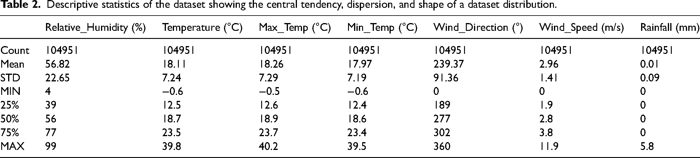
In this work, we explore the potential of using ARIMA models to forecast wind speed using a data captured from a meteorological station located in Palestine for a duration of 2 years—January 1, 2021 to December 31, 2022. The collected wind data were constantly logged at an altitude of 20 m by a rotating cup generator anemometer installed in Jabal Al-Mukabber's village nearby east Jerusalem with an accuracy of (3%), and the calibration was performed by a linear regression uncertainty with a percentage of 0.2% to 5.0%. As shown in Table 1, the dataset contained seven variables. The captured records have a frequency of 10 min. Some preliminary preprocessing steps were applied in order to process the data, the original data were thoroughly reviewed for errors, and few null and missing values were filled by taking the average of five previous values. Also, a statistical analysis was used to clarify the main attributes of the time series data as shown in Table 2, we found out that each attribute had (104951) readings. The average values of the relative humidity were found to be 56.82%, the mean temperature (18.11°C), mean maximum temperature (18.26°C), mean minimum temperature (17.97°C), and mean rainfall (0.01 mm). The mean value of wind speed was 2.96 m/s with wind direction values ranging from 0 to 360 degrees, the wind direction's mean showed that the overall wind direction was southwest. The standard deviation of the time series was also found to check the stationarity of the dataset. Besides, 75% of the values are less than or equal to (3.8 m/s), which is a reasonable value that is suitable for installing small wind turbines, about 75% of the air temperature values were below 24°C, 75% of wind direction was originated from the northwest and 50% nearly to the south. The peak value of wind speed was (11.9 m/s), while the peak value of the air temperature was found to be around (40°C). A graphical representation of the first 5 days of January 2021 was presented in Figure 1 to provide a clear visualization of the wind speed values and their variation.

Figure 1.

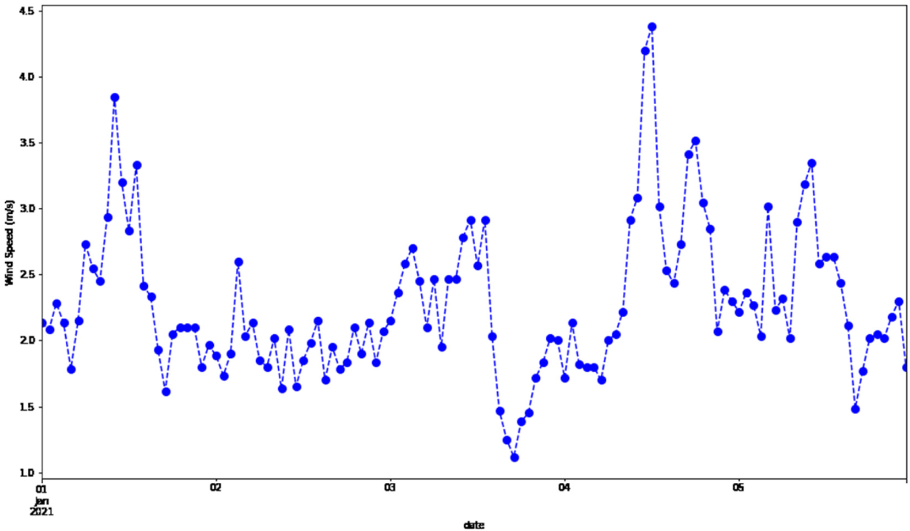
An example of five-day time series wind speed data.

Table 1.

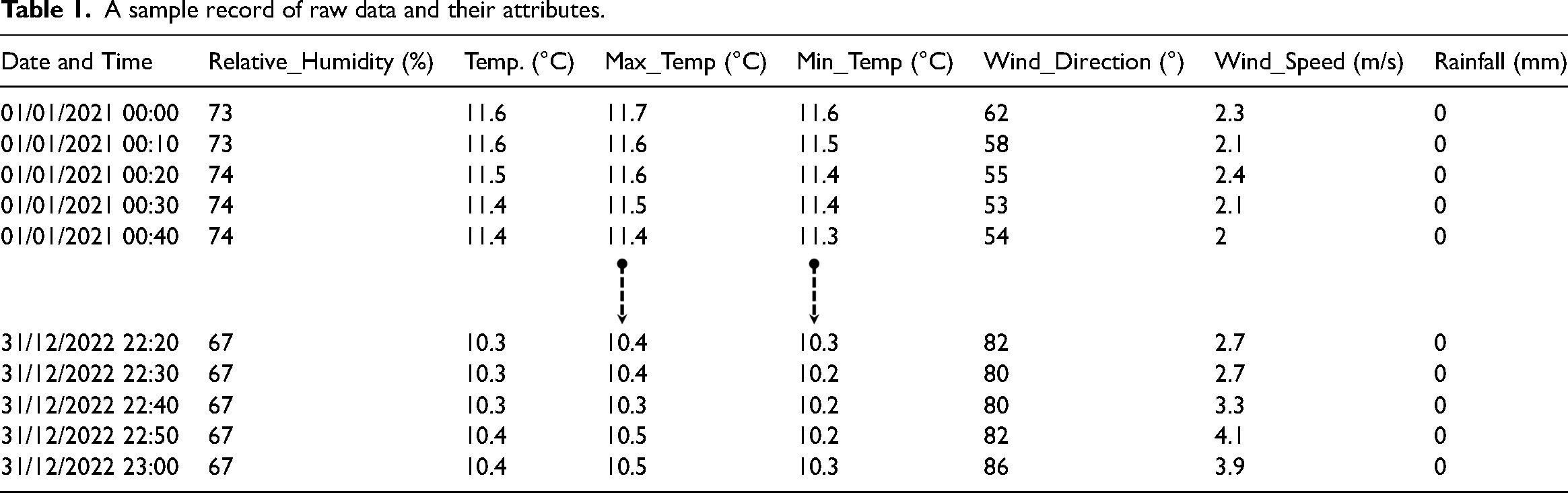
A sample record of raw data and their attributes.

Table 2.

Descriptive statistics of the dataset showing the central tendency, dispersion, and shape of a dataset distribution.

	Relative_Humidity (%)	Temperature (°C)	Max_Temp (°C)	Min_Temp (°C)	Wind_Direction (°)	Wind_Speed (m/s)	Rainfall (mm)
Count	104951	104951	104951	104951	104951	104951	104951
Mean	56.82	18.11	18.26	17.97	239.37	2.96	0.01
STD	22.65	7.24	7.29	7.19	91.36	1.41	0.09
MIN	4	−0.6	−0.5	−0.6	0	0	0
25%	39	12.5	12.6	12.4	189	1.9	0
50%	56	18.7	18.9	18.6	277	2.8	0
75%	77	23.5	23.7	23.4	302	3.8	0
MAX	99	39.8	40.2	39.5	360	11.9	5.8

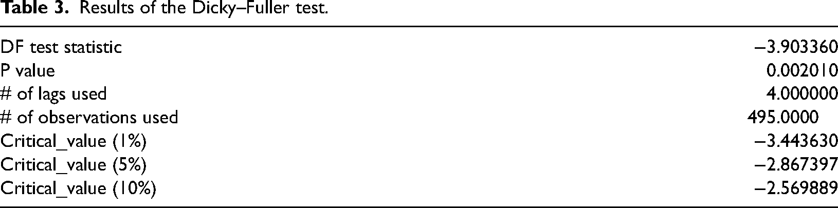
By referring to the Box–Jenkins methodology for proposing an ARIMA model, the data stationarity and seasonality criteria must be carried out. Regarding the seasonality criterion for the considered wind speed time series dataset, there were no peaks at seasonal frequencies, and thus, no trends for seasonal wind speed which reveals no random variations in the wind speed data as illustrated in Figures 1 and 2. Also, referring to Figure 2, it is clearly shown that the trend and residuals reveal that the time series is stationary. In addition to that, by referring to Table 3, which shows the results of the Dicky–Fuller test; a widely used unit root test method to evaluate the stationarity of a time series, the test values clearly indicate that the wind speed data had no unit roots and can be characterized as a stationary time series. As a consequence, the null hypothesis was rejected at a 95% level of confidence (Dickey–Fuller test: −3.903, P < 0.05%).

Figure 2.

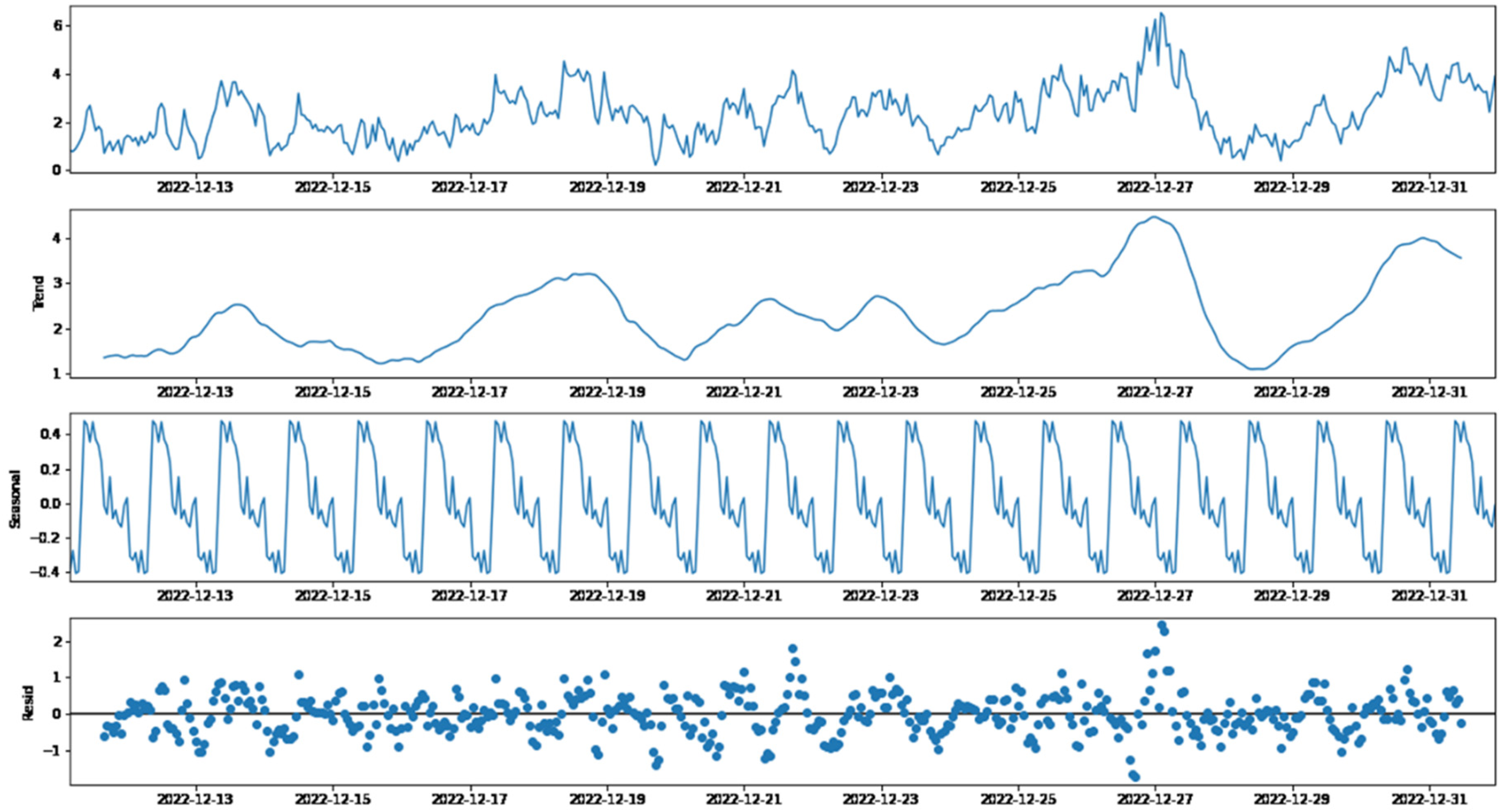
Decomposition example of the time series into trend, seasonal, and residual components.

Table 3.

Results of the Dicky–Fuller test.

DF test statistic	−3.903360
P value	0.002010
# of lags used	4.000000
# of observations used	495.0000
Critical_value (1%)	−3.443630
Critical_value (5%)	−2.867397
Critical_value (10%)	−2.569889

In this regard, ACF and PACF are two measures that are typically used to find the association between current and past values of a series and to indicate which past values are the most valuable in predicting the future ones. With these measures, researchers can determine the order of processes in the ARIMA model. The autocorrelation of stationary data might reduce to zero almost quickly, whereas for a nonstationary time series, it is significantly at a distance from zero for many times. Some samples of ACF and PACF of the observed time series are presented in Figure 3, and as it is observed, the autocorrelation function (ACF) decays quickly to zero and there are no clear patterns in both plotted samples. As a consequence, the considered time series dataset seems to be stationary.

Figure 3.

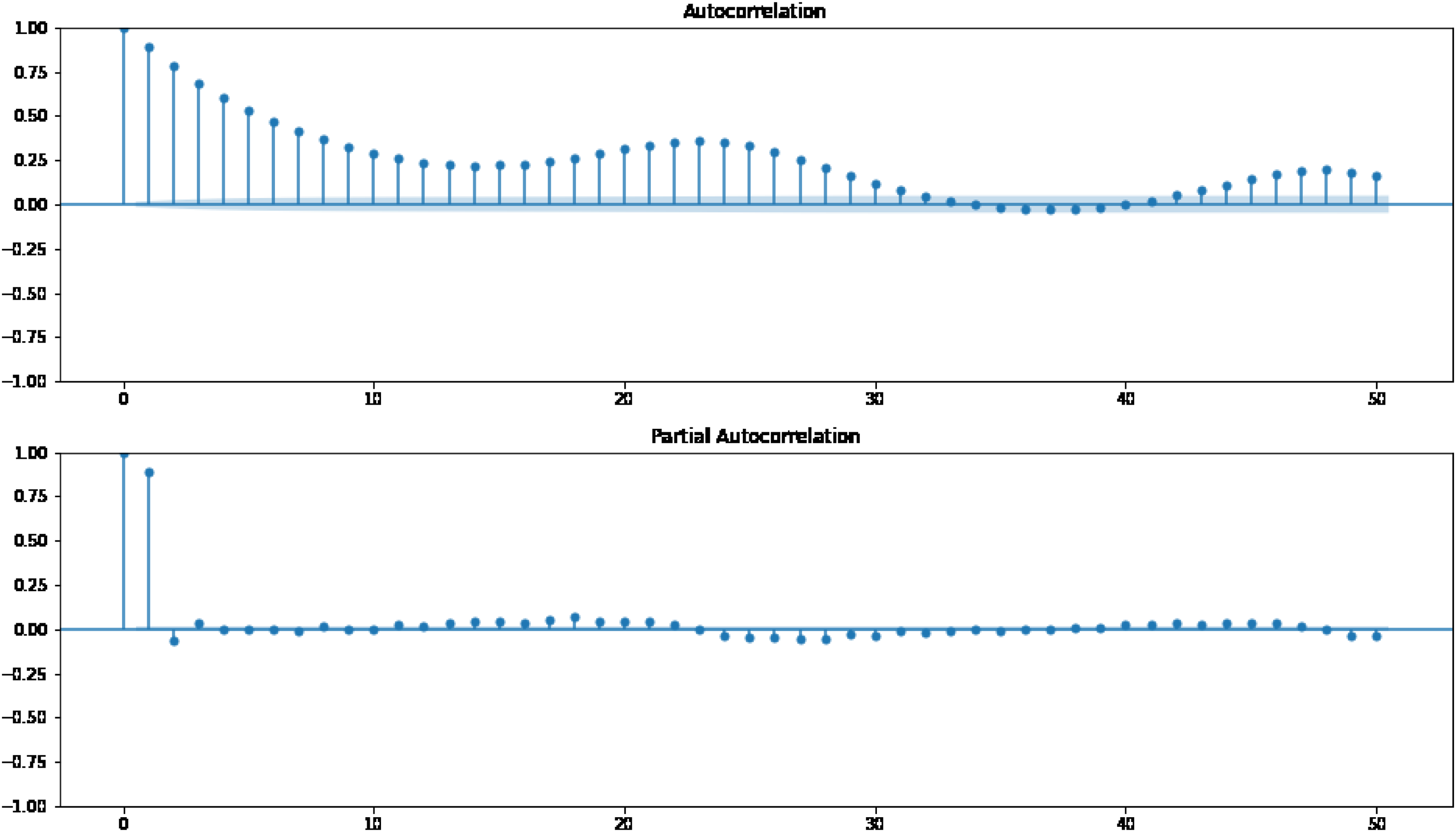
Plots of ACF and PACF.

Working with stationary time series, a set of ARIMA (p, d, q) models was constructed by changing the values of p and q with integers ranging [0–4]. The maximum value is 5, which was selected to keep frugality in mind. Among the possible constructed models, the optimal model was detected after capability check. The analysis of ACF and PACF functions did not show the accurate values of p and q. But as the scientific literature argued, the d parameter mostly takes the value 0, in some scenarios it might also take the value 1 to avoid the weak stationarity cases. To find the optimal model, the parameters p and q can be assigned various values. For each pair of values, a new model was constructed.

Figure 4 illustrates the flowchart of ARIMA model. The time series dataset is first checked to determine whether it is stationary or nonstationary. This test can be made by utilizing several methods such as data visualization, summary statistics, and statistical methods. If the data is stationary, the plots of ACF and PACF will be created to find patterns in the data and to identify the occurrence of AR and MA components in the residuals. If the dataset is nonstationary, a new step is necessary to make the series stationary by converting a stationary time series by using the differencing technique. Differencing the time series is the change between a set of consecutive data points in the series by subtracting the current value from its predecessor, or from a lagged value. Next, the estimation of the optimal parameters for the ARIMA model is done to identify the best fit ARIMA model on the fly, and then check the accuracy of the model using several performance metrics. Finally, the model will be built and validated by making a comparative analysis between actual and predicted values in the validation sample.

Figure 4.

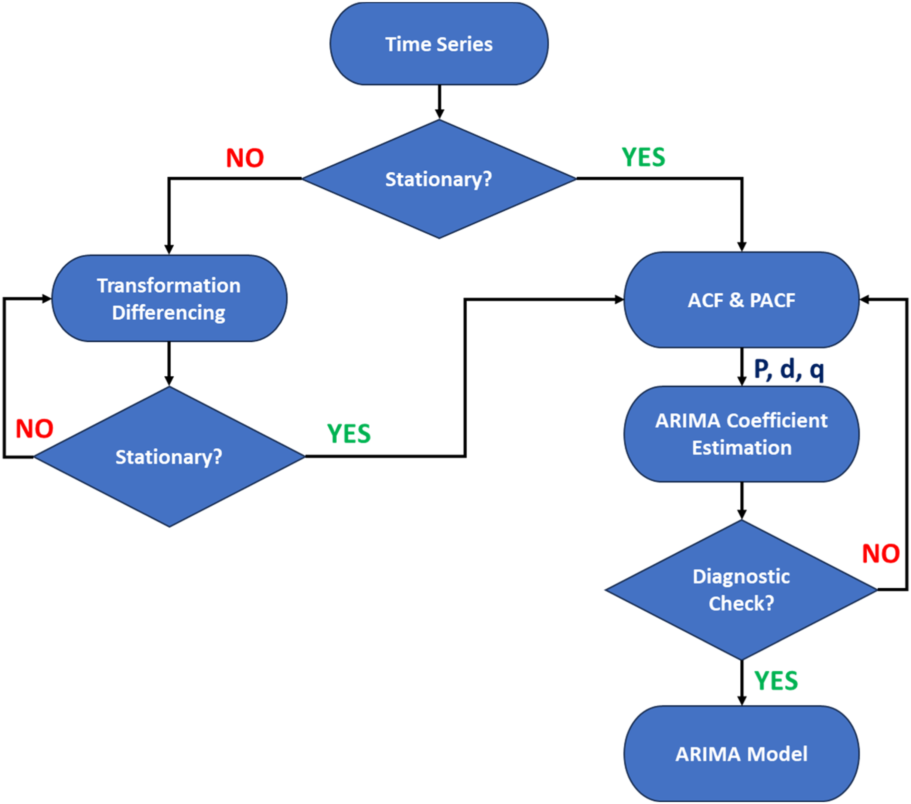
Flowchart of the ARIMA time series forecasting model (Mani and Volety, 2021).

Performance metrics of wind speed forecasting

RMSE

As given in equation (4), the RMSE is the most widely applied performance metric to estimate the average value of the prediction error by calculating the differences between predicted and observed/actual values.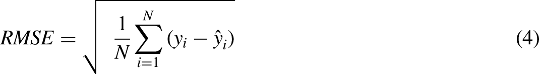

R M S E = \sqrt{\frac{1}{N} \sum_{i = 1}^{N} (y_{i} - {\hat{y}}_{i})}

(4)

where

y_{i}, {\hat{y}}_{i}

, N is the actual value, the predicted value, and the number of samples, respectively. Small values of RMSE imply that the suggested forecasting model provides better accuracy (Hyndman and Athanasopoulos, 2018).

MAE

As indicated by equation (5), the MAE represents the mean of absolute differences between actual and predicted values; it corresponds to the estimated level of absolute error.

\frac{1}{N} \sum_{i = 1}^{N} | y_{i} - {\hat{y}}_{i} |

(5)

where

{\hat{y}}_{i}

y_{i}

, and N is the predicted value, actual value, and the number of samples or prediction points, respectively. Smaller values of MAE mean that the suggested forecasting model gives better accuracy (Hyndman and Athanasopoulos, 2018).

R-square

The coefficient of determination or R-square (R²) (equation (6)) represents the level of correlation between actual and predicted values; it can be described as the variance of the dependent variable which is predicted from the set of independent variables. It is mainly used in time series datasets having large amplitudes.

R^{2} = 1 - \frac{\sum_{i = 1}^{N} {(y_{i} - {\hat{y}}_{i})}^{2}}{\sum_{i = 1}^{N} {(y_{i} - \bar{y})}^{2}}, f o r \bar{y} = \frac{1}{N} \sum_{i = 1}^{N} y_{i}

(6)

where

y_{i}, \bar{y}

{\hat{y}}_{i}

, N is the actual value, the average value, the predicted value, and the number of samples, respectively. As R² value approaches 1, it indicates that the model gives higher forecasting accuracy (Dabbaghiyan et al., 2016).

Results and discussions

To find the optimal values of the ARIMA parameters for the study site, several experiments were conducted by adjusting the values of p and q [0–4], for each pair, a new model was constructed and validated. As it is clearly observed from Figure 2, the plot provides a time series data that exhibits a repetitive behavior with visible and regular recurring cycles. This periodic behavior assures that the underlying process of interest can be regular, and the frequency of oscillations that describes the behavior of the series will help to identify it. The series mainly shows two types of ﬂuctuations: sinusoidal waves with bottom and top peaks and a slower frequency that seems to be repeated periodically. Typically, nonstationary data cannot be modeled or predicted. The results extracted from nonstationary time series can be inconsistent or unreliable, because they can relate two variables where neither of them exists. To determine the orders p and q, the plots of both ACF and partial autocorrelation function (PACF) were examined as illustrated in Figure 3. These plots clearly show that the values tend to deteriorate quickly to zero without clear patterns, which is also verified using the Dicky–Fuller test results, which confirms stationarity nature of the dataset. The PACF plots provide that the AR (2) model is more suitable for the observed data, because of the cut-off at lag 2.

After accomplishing the stationarity test of the time series, the next step is to check whether AR or MA terms are needed to correct any autocorrelation required to fit the ARIMA model. The analysis of autocorrelation and partial autocorrelation did not give the correct values of the parameters p and q. However, referring to the literature, the d parameter should take either 0 or 1 for stationary time series. The zero values differencing models (d = 0) were also presented in the results (Table 4) to confirm that these models can provide higher prediction errors compared to d = 1. Consequently, the best model was found by assigning different values [0–4] for both p and q parameters. A new model was built for each pair of values, and some statistical performance metrics were used to compare between the assigned AR and MA values (p and q parameters). The best forecasting wind speed model was found to be ARIMA (2, 1, 2) which means that; an autoregressive AR(2) process in which the current observation value is based on the previous two lagged observations, the weak stationarity of the wind speed time series was avoided by taking the first order differencing of the raw observations, that is, subtraction of the current value with its previous time step value, and moving average MA(2) incorporates that the dependency between the observation and the residual error from a second order moving average is applied to the lagged observations.

Table 4.

Experimental results of various error metrics to identify the optimal parameters for the ARIMA (p, d, q) model.

Parameters	RMSE	MAE	R-square	Parameters	RMSE	MAE	R-square
(2, 1, 2)	1.738	1.583	0.762	(2, 0, 2)	1.975	1.811	0.741
(4, 1, 4)	1.748	1.593	0.724	(2, 0, 3)	1.975	1.811	0.741
(1, 1, 2)	1.747	1.593	0.760	(4, 0, 2)	1.973	1.811	0.687
(2, 1, 1)	1.747	1.594	0.760	(3, 0, 0)	1.976	1.811	0.738
(1, 1, 1)	1.749	1.595	0.760	(1, 0, 2)	1.977	1.812	0.734
(2, 1, 3)	1.751	1.598	0.757	(2, 0, 1)	1.972	1.813	0.757
(1, 1, 4)	1.759	1.6	0.753	(3, 0, 4)	1.983	1.815	0.671
(3, 1, 2)	1.76	1.602	0.752	(1, 0, 1)	1.977	1.819	0.753
(3, 1, 4)	1.768	1.609	0.587	(1, 0, 0)	1.977	1.819	0.753
(3, 1, 1)	1.77	1.611	0.748	(2, 0, 0)	1.978	1.819	0.753
(3, 1, 3)	1.782	1.615	0.576	(2, 0, 4)	1.985	1.822	0.724
(4, 1, 3)	1.783	1.635	0.661	(1, 0, 4)	1.985	1.823	0.724
(0, 0, 1)	1.915	1.725	0.200	(4, 1, 2)	2.078	1.902	0.005
(0, 0, 0)	1.915	1.728	0.000	(2, 1, 4)	2.081	1.907	0.158
(0, 0, 2)	1.916	1.732	0.194	(0, 1, 2)	2.091	1.917	0.200
(0, 0, 4)	1.922	1.754	0.462	(0, 1, 3)	2.092	1.918	0.225
(0, 0, 3)	1.922	1.755	0.403	(1, 1, 3)	2.092	1.918	0.203
(4, 0, 4)	1.935	1.77	0.674	(4, 1, 0)	2.102	1.931	0.197
(3, 0, 2)	1.971	1.806	0.684	(3, 1, 0)	2.105	1.932	0.050
(4, 0, 3)	1.971	1.806	0.684	(4, 1, 1)	2.103	1.933	0.223
(1, 0, 3)	1.974	1.809	0.740	(2, 1, 0)	2.107	1.933	0.019
(4, 0, 0)	1.974	1.809	0.743	(0, 1, 4)	2.108	1.939	0.394
(4, 0, 1)	1.974	1.81	0.741	(0, 1, 1)	2.172	2.004	0.000
(3, 0, 1)	1.974	1.81	0.741	(1, 1, 0)	2.182	2.014	0.181
(3, 0, 3)	1.972	1.81	0.687	(0, 1, 0)	2.197	2.031	0.197

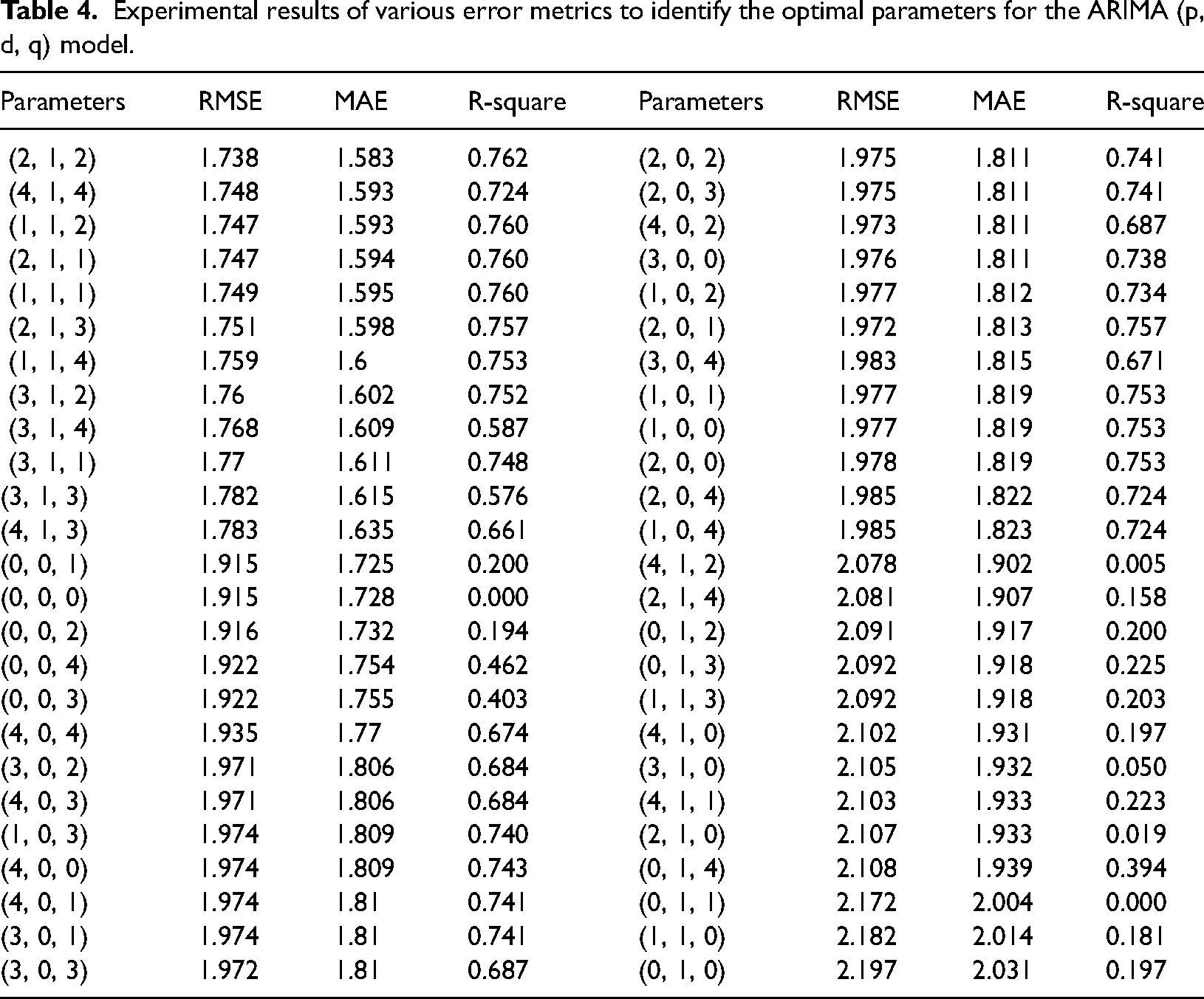
Table 4 shows the experimental results of various error metrics to identify the optimal parameters for the ARIMA model. It is clearly shown that the highest value for both p and q are 4 and 4, respectively. Since the model should give high prediction accuracy with the lowest errors and should be the easiest one. When p and q take larger values, the model becomes more complex to calculate and analyze. The best forecasting model was selected based on accuracy and performance. To evaluate the models and select the best one that describes the wind speed data accurately, several accuracy methods were employed. The results presented in Table 4 show that ARIMA (21,2) gives the most accurate estimation with minimal RMSE (1.74), minimal MAE (1.58), and higher R² (0.76) values. It is achieved when the autoregressive process is based on the previous two lagged observations, and the moving average process relates the dependency between the observations and the residual errors using a second-order moving average applied to the lagged observations. By referring to Table 4, it was found the MAE values for all models ranging from 1.58 to 2.03, where the RMSE values come to be in the range of 1.73 to 2.19, and the values of R² ranged from 0 to 0.76. Furthermore, ARIMA (4, 1, 4) gives good wind speed prediction with lower errors. However, ARIMA (2, 1, 2) has a simpler construction and the difference of errors is not big enough to choose a more complex model. A comparison of the actual wind speed data with the best ARIMA (2, 1,2) model for three days is presented in Figure 5. It is observed that both curves are matched and the ARIMA (2, 1, 2) model is well representing the observed wind speed pattern. The training dataset predicted by the model described well the actual training wind speed values with an overestimation for values less than 3 m/s and underestimation of wind speed for values greater than 3 m/s, while the ARIMA model failed to describe the test wind speed dataset.

Figure 5.

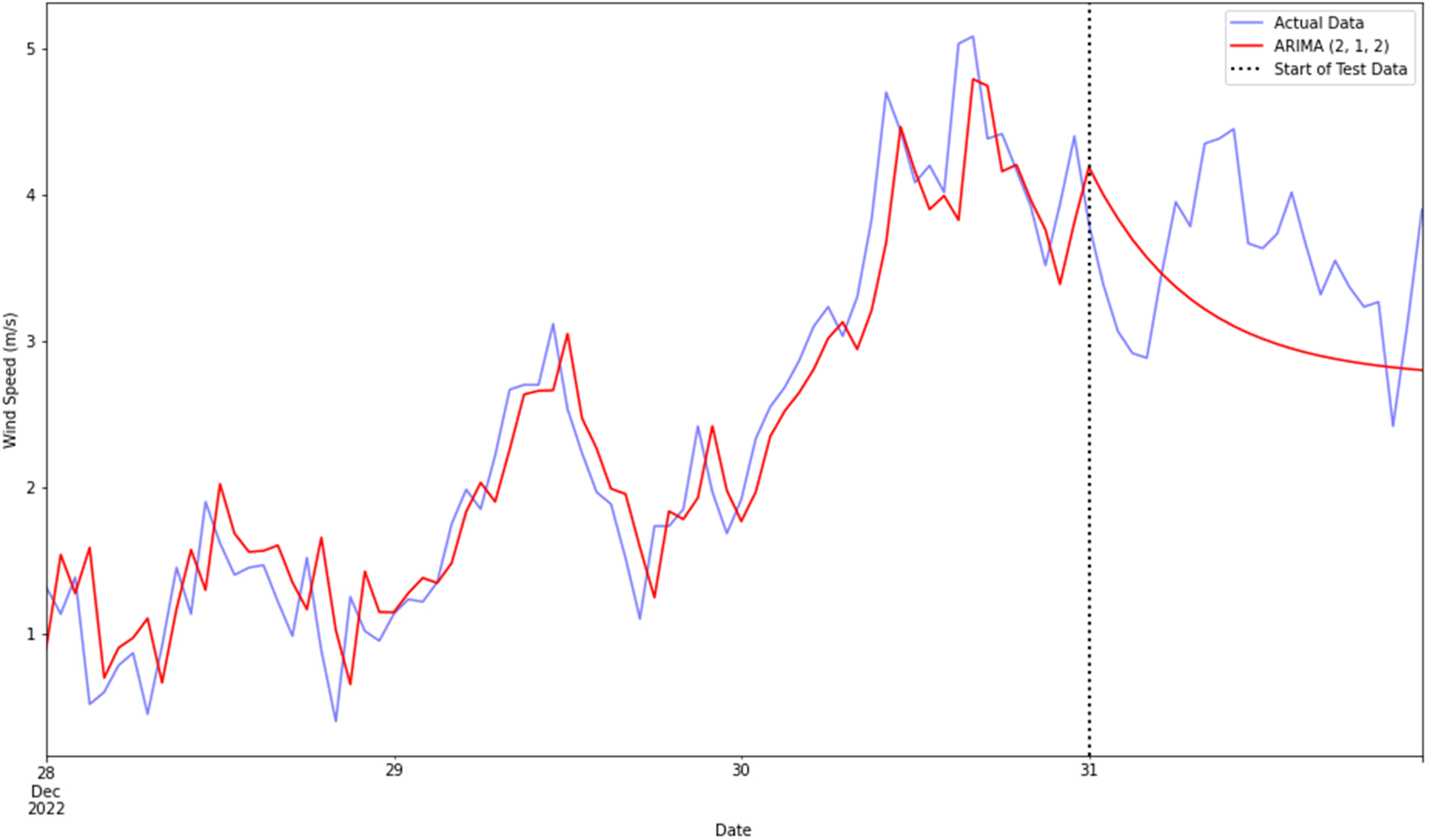
Wind speed forecasting of ARIMA (21,2) versus actual data.

To sum up, the performance of the ARIMA models was estimated using wind speed dataset using various evaluation metrics. RMSE, MAE, and R² were used to assess the models, and the results have shown that ARIMA model achieves acceptable forecasting accuracy of wind speed in east Jerusalem as compared with similar studies from the literature.

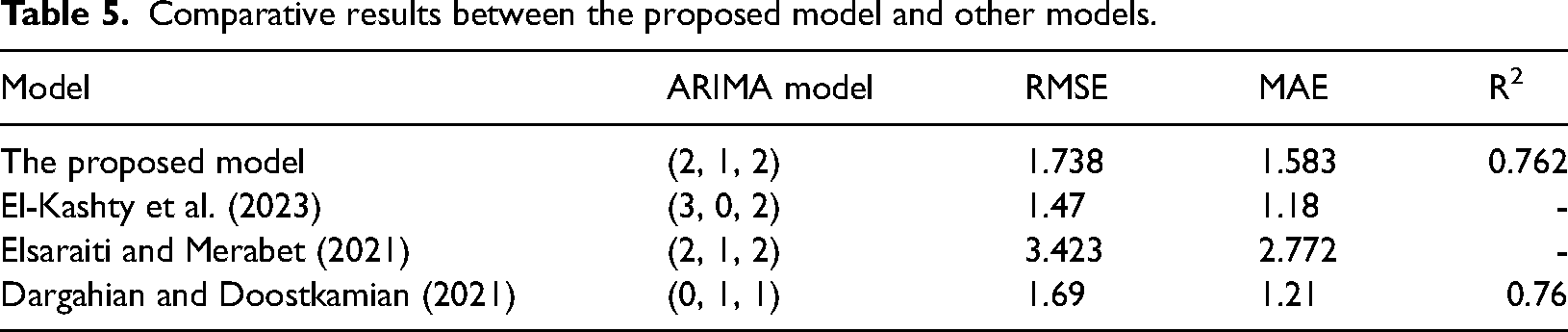
As it is clearly emphasized in the literature, the analysis of wind speed is site-dependent; that is, it depends on the intrinsic nature of the wind and its characteristics. Nevertheless, to study how the proposed model behaves compared to other similar studies, Table 5 summarizes the results along with some of those presented in the literature. El-Kashty et al. (2023) modeled the wind speed for short and long term in Ras-Gharib, Egypt by using several time-series forecasting methods. The authors used daily wind speed data from January 2017 to December 2021. Among the compared methods, ARIMA (3, 0, 2) provided the best statistical performance with RMSE (1.47) and MAE (1.18). Elsaraiti and Merabet (2021) studied the effectiveness of predicting wind speed for Halifax region, Canada. They used a short time series wind data from 1 May 2021 to 20 June 2021, and the results have shown that ARIMA (2, 1, 2) provided the best statistical performance with RMSE (3.423) and MAE (2.772). In Iran, Helmand Basin, wind speed spatial patterns assessment and forecasting models were studied by Dargahian and Doostkamian (2021), daily data from 1990 to 2018 collected from seven stations in Helmand region were used to conduct the study. The authors concluded that the statistical performance of ARIMA (0, 1, 1) model was more accurate for Zahak station than others with values 1.69, 1.21, and 0.76, for RMSE, MAE, and R², respectively. As shown in the table, the statistical performance of ARIMA (2, 1, 2) model presented in this work provides reasonable values when compared to that in the literature.

Table 5.

Comparative results between the proposed model and other models.

Model	ARIMA model	RMSE	MAE	R²
The proposed model	(2, 1, 2)	1.738	1.583	0.762
El-Kashty et al. (2023)	(3, 0, 2)	1.47	1.18	-
Elsaraiti and Merabet (2021)	(2, 1, 2)	3.423	2.772	-
Dargahian and Doostkamian (2021)	(0, 1, 1)	1.69	1.21	0.76

These results give a baseline that allows to establishing the optimal ARIMA structure and the length of the input period in the study site. The conducted study revealed that the identification of the optimal ARIMA model can give a significant improvement in accuracy compared to the casual structures for three days ahead forecast. As indicated in the literature, the ARIMA model can produce better results when applied to small datasets. However, for large datasets, to obtain better forecasts, it is highly recommended to propose a couple of ARIMA models with other effective methods combined together as hybrid models or using models generated based on deep learning paradigms.

Conclusion

In this work, we developed and evaluated a set of ARIMA models for wind speed forecasting using a data captured from a meteorological station located in east Jerusalem, Palestine for a duration of 2 years—January 1, 2021 to December 31, 2022. To find the optimal values of ARIMA parameters (p, d, q), a set of experiments were conducted and the model's forecasting accuracy was evaluated using three metrics: RMSE, MAE, and the coefficient of determination (R²). The results have shown that ARIMA (21,2) emerges as the most accurate ARIMA structure and the length of the input period demonstrate superior estimation with minimal RMSE (1.74), minimal MAE (1.58), and higher R² (0.76) values.

The output of this work exhibits a number of points to consider (a) it should be indicated that with the tremendous growing of wind-based applications, power utilities in Palestine have to integrate a variety of renewable energy systems, an accurate estimate of wind speed plays a vital role in socioeconomic benefits resulting from an appropriate power grid supervision in the Palestinian territories; (b) this study can help in ease managing of wind farm programs and operations, for the obtained ARIMA models can not only get the best accuracy when compared with existing models but also can be simply calculated; and (c) the findings suggest that ARIMA models remain effective for short-term wind speed prediction and could aid decision-makers in Palestine to discover the local wind potential and offer some insights into the feasibility of wind speed forecasting for sustainable energy solutions.

In the future research work, we will conduct a deep analysis to explore the behavior of the ARIMA model per season, and explore hybrid models that combine ARIMA with other forecasting techniques to further improve the performance under different conditions. Another line of research would be to obtain other wind speed datasets from different measurement sites in Palestine and make a comparative analysis.

Footnotes

Declaration of conflicting interests

The authors declared no potential conflicts of interest with respect to the research, authorship, and/or publication of this article.

Funding

The authors received no financial support for the research, authorship, and/or publication of this article.

ORCID iD

Saeed Salah

References

Abdallah

Çamur

(2022) Assessing the potential of wind energy as sustainable energy production in Ramallah, Palestine. Sustainability 14: 9352.

Adebiyi

Adewumi

Ayo

(2014) Comparison of ARIMA and artificial neural networks models for stock price prediction. Journal of Applied Mathematics 2014: 614342.

Alsamamra

Salah

Shoqeir

, et al. (2022) A comparative study of five numerical methods for the estimation of Weibull parameters for wind energy evaluation at eastern Jerusalem, Palestine. Energy Reports 8: 4801–4810.

Box

GEP

Jenkins

(1970) Time Series Analysis: Forecasting and Control. San Francisco: Holden-Day.

Brown

Katz

Murphy

(1984) Time series models to simulate and forecast wind speed and wind power. Journal of Climate and Applied Meteorology 23: 1184–1195.

Cadenas

Rivera

(2007) Wind speed forecasting in the south coast of Oaxaca, México. Renewable Energy 32: 2116–2128.

Chandra

Goyal

Gupta

(2021) Evaluation of deep learning models for multi-step ahead time series prediction. IEEE Access 9: 83105–83123.

Chen

Tang

Zeng

, et al. (2022) Short-term wind speed forecasting based on long short-term memory and improved BP neural network. International Journal of Electric Power Energy Systems 134: 107365.

Chodakowska

Nazarko

, et al. (2023) ARIMA Models in solar radiation forecasting in different geographic locations. Energies 16: 5029.

10.

Contreras

Espínola

Nogales

, et al. (2003) ARIMA Models to predict next-day electricity prices. IEEE Transactions on Power Systems 18: 1014–1020.

11.

Dabbaghiyan

Fazelpour

Abnavi

, et al. (2016) Evaluation of wind energy potential in province of Bushehr, Iran. Renewable and Sustainable Energy Reviews 55: 455–466.

12.

Dargahian

Doostkamian

(2021) Assessment and forecasting spatial pattern changes of dust and wind speed using ARIMA and ANNs model in Helmand basin, Iran. Journal of Earth System Science 114: 1–11.

13.

Demolli

Dokuz

Ecemis

, et al. (2019) Wind power forecasting based on daily wind speed data using machine learning algorithms. Energy Conversion and Management 198: 111823.

14.

Dimri

Ahmad

Sharif

(2020) Time series analysis of climate variables using seasonal ARIMA approach. Journal of Earth System Science 129: 149–158.

15.

Wang

Yang

, et al. (2019) A novel hybrid model for short-term wind power forecasting. Applied Soft Computing 80: 10–17.

16.

Dumitru

Gligor

(2017) Daily average wind energy forecasting using artificial neural networks. Procedia Engineering 181: 829–836.

17.

El-Kashty

Daoud

El-Araby

(2023) Forecasting of short-term and long-term wind speed of Ras-Gharib using time series analysis. International Journal of Energy Research 13: 258–272.

18.

Elsaraiti

Merabet

(2021) A comparative analysis of the ARIMA and LSTM predictive models and their effectiveness for predicting wind speed. Energies 14: 6782.

19.

Global Wind Energy Council (2021) Global Wind Report 2021. Brussels, Belgium: Global Wind Energy Council.

20.

Global Wind Energy Council (2022) Global Wind Report 2022. Brussels, Belgium: Global Wind Energy Council.

21.

Grigonytė

Butkevičiūtė

(2016) Short-term wind speed forecasting using ARIMA model. Energetika 62: 17–26.

22.

Hamed

Flamm

Azraq

(2012) Renewable energy in the Palestinian territories: Opportunities and challenges. Renewable and Sustainable Energy Reviews 16: 1082–1088.

23.

Hanifi

Liu

Lin

, et al. (2020) A critical review of wind power forecasting methods—past, present and future. Energies 13: 3764.

24.

Hong

Satriani

TRA

(2020) Day-ahead spatiotemporal wind speed forecasting using robust design-based deep learning neural network. Energy 209: 118441.

25.

Hoolohan

Tomlin

Cockerill

(2018) Improved near surface wind speed predictions using Gaussian process regression combined with numerical weather predictions and observed meteorological data. Renewable Energy 126: 1043–1054.

26.

Wang

(2015) Short-term wind speed prediction using empirical wavelet transform and Gaussian process regression. Energy 93: 1456–1466.

27.

Hur

(2021) Short-term wind speed prediction using extended Kalman filter and machine learning. Energy Reports 7: 1046–1054.

28.

Hussin

Yusof

Jamaludin

, et al. (2021) Forecasting wind speed in peninsular Malaysia: An application of ARIMA and ARIMA-GARCH models. Pertanika Journal of Science Technology 29: 88–96.

29.

Hyndman

Athanasopoulos

(2018) Forecasting: principles and practice, 2nd ed. Melbourne: OTexts.

30.

Ibrik

(2019) Techno-economic analysis of wind energy resources based on real measurements in West Bank–Palestine. International Journal of Energy Economics and Policy 9: 26–32.

31.

Juaidi

Abdallah

Ayadi

, et al. (2022a) Wind energy in Jordan and Palestine: Current status and future perspectives. Renewable Energy Products Distribution 13: 37–45.

32.

Juaidi

Montoya

Ibrik

, et al. (2022b) An overview of renewable energy potential in Palestine. Renewable and Sustainable Energy Reviews 65: 943–960.

33.

Kitaneh

Alsamamra

Aljunaidi

(2012) Modeling of wind energy in some areas of Palestine. Energy Conversion and Management 62: 64–69.

34.

Kosanoglu

(2022) Wind speed forecasting with a clustering-based deep learning model. Applied Science 12: 13031.

35.

Herdem

Nathwani

, et al. (2023a) Methods and applications for artificial intelligence, big data, internet of things, and blockchain in smart energy management. Energy and AI 11: 100208.

36.

Shen

, et al. (2023b) Exploring time series models for wind speed forecasting: A comparative analysis. Energies 16: 7785.

37.

Liu

Sun

Liu

, et al. (2019) On wind speed pattern and energy potential in China. Applied Energy 236: 867–876.

38.

Liu

Tian

(2012) Comparison of two new ARIMA-ANN and ARIMA-Kalman hybrid methods for wind speed prediction. Applied Energy 98: 415–424.

39.

Mani

Volety

(2021) A comparative analysis of LSTM and ARIMA for enhanced real-time air pollutant levels forecasting using sensor fusion with ground station data. Cogent Engineering 8: 1936886.

40.

Mantalos

Mattheou

Karagrigoriou

(2010) Forecasting ARMA models: A comparative study of information criteria focusing on MDIC. Journal of Statistical Computation and Simulation 80: 61–73.

41.

Manwell

McGowan

Rogers

(2010) Wind Energy Explained: Theory, Design and Application. Hoboken, NJ: John Wiley & Son.

42.

Liu

(2018) Wind speed forecasting method based on deep learning strategy using empirical wavelet transform, long short-term memory neural network and Elman neural network. Energy Conversion and Management 156: 498–514.

43.

Palestinian Central Bureau of Statistics (PCBS). Available online: http://www.pcbs.gov.ps/ (Online; last accessed on February 29, 2024).

44.

Sahoo

Jha

Singh

, et al. (2019) Long short-term memory (LSTM) recurrent neural network for low-flow hydrological time series forecasting. Acta Geophysics 67: 1471–1481.

45.

Salah

Alsamamra

Shoqeir

(2022) Exploring wind speed for energy considerations in eastern Jerusalem-palestine using machine-learning algorithms. Energies 15: 2602.

46.

Salman

Heryadi

Abdurahman

, et al. (2018) Weather forecasting using merged long short-term memory model (LSTM) and autoregressive integrated moving average (ARIMA) model. Journal of Computer Science 14: 930–938.

47.

Shang

Chen

, et al. (2022) Short-term wind speed forecasting system based on multivariate time series and multi-objective optimization. Energy 238: 122024.

48.

Shoaib

Siddiqui

Rehman

, et al. (2019) Assessment of wind energy potential using wind energy conversion system. Journal of Cleaner Production 216: 346–360.

49.

Sun

Jin

(2022) A hybrid approach to multi-step, short-term wind speed forecasting using correlated features. Renewable Energy 186: 742–754.

50.

Torres

García

Blas

, et al. (2005) Forecast of hourly average wind speed with ARMA models in Navarre (Spain). Solar Energy 1: 65–77.

51.

Tyass

Bellat

Raihani

, et al. (2022) Wind speed prediction based on seasonal ARIMA model. International Conference on Energy and Green Computing 336: 28–33.

52.

Zeng

Sun

Farnham

(2020) Skillful statistical models to predict seasonal wind speed and solar radiation in a Yangtze river estuary case study. Scientific Reports 10: 8597.

Performance analysis of ARIMA Model for wind speed forecasting in Jerusalem,Palestine

Abstract

Keywords

Introduction

Related work

ARIMA model

AR

MA

ARIMA

Dataset and methodology

Performance metrics of wind speed forecasting

RMSE

MAE

R-square

Results and discussions

Conclusion

Footnotes

Declaration of conflicting interests

Funding

ORCID iD

References