Sage Journals: Discover world-class research

Abstract

Smart homes are at the forefront of sustainable living, utilizing advanced monitoring systems to optimize energy consumption. However, these systems frequently encounter issues with anomalous data such as missing data, redundant data, and outliers data which can undermine their effectiveness. In this paper, an artificial neural network (ANN)-based approach for data imputation is specifically designed to deal with the anomalies in smart home energy consumption datasets. Our research harnesses the power of ANNs to model intricate patterns within energy consumption data, enabling the accurate imputation of missing values while detecting and rectifying anomalous data. This approach not only enhances the completeness of the data but also augments its overall quality, ensuring more reliable results. To evaluate the effectiveness of our ANN-based imputation method, comprehensive experiments were conducted using real-world smart home energy consumption datasets. Our findings demonstrate that this approach outperforms traditional imputation techniques like mean imputation and median imputation in terms of accuracy. Furthermore, it showcases adaptability to diverse smart home scenarios and datasets, making it a versatile solution for improving data quality. In conclusion, this study introduces an advanced data imputation technique based on ANNs, tailor-made for addressing anomalies in smart home energy consumption data. Beyond merely filling data gaps, this approach elevates the dataset's reliability and completeness, thereby facilitating a more precise analysis of energy consumption and supporting informed decision-making in the context of smart homes and sustainable energy management. Ultimately, the proposed method has the potential to contribute considerably to the ongoing evolution of smart home technologies and energy conservation efforts.

Keywords

Artificial neural networks data anomalies energy consumption missing data imputation smart home

Introduction

Smart homes play a pivotal role in the global pursuit of energy efficiency and sustainability, and the reliability of data generated by these systems is of paramount importance. Day by day limitless data are being generated in the smart home environment with the installation of sensors and smart meters (Himeur et al., 2021). The electricity consumption of smart buildings/homes plays a vital role in energy management and this energy management should be further enhanced (Aguilar et al., 2021). This energy management helps to improve the smart grid's functionality in various aspects such as demand-side management, thwarting blackouts, and high-quality power to the consumers (Purna Prakash et al., 2022a; 2022b). But to achieve these functionalities, the energy consumption data should not contain any anomalies (Purna Prakash and Pavan Kumar, 2022c). Some of the most commonly occurring anomalies in energy consumption are missing data, redundant data, and outliers (Purna Prakash and Pavan Kumar, 2021, Purna Prakash and Pavan Kumar, 2022d). Energy data digitalization has created new opportunities to find out such anomalies easily (Leiria et al., 2021). The identification of missing data and its behavior further the imputation leading to better energy analytics (Wang et al., 2021, Purna Prakash and Pavan Kumar, 2022e). There are different strategies such as single and multiple imputations for imputing the missing data (McCombe et al., 2022). It is always desired to recover the missed data to maintain the reliability of monitoring applications in industries with the Internet of Things (IoT) (Liu et al., 2020). An alternate learning and multivariate imputation by chained equations strategies are used to impute the missing data further to maintain data integrity (Lai et al., 2020, Wu et al., 2022). Machine learning techniques are helpful in handling data anomalies in smart home power consumption (Purna Prakash and Pavan Kumar, 2022d). Along with these techniques, a complete survey is executed to understand the applicability of missing data imputation techniques (Miao et al., 2023). The literature works on the imputation of data using various techniques are discussed as follows.

Novel imputation methods for different types of missing data imputation were discussed in the intensive care unit's data (Venugopalan et al., 2019). A data imputation approach relied on denoising autoencoder (DAE) with the k-nearest neighbor (KNN) was implemented to complete the pre-imputation task, and further, the imputation is optimized by (Psychogyios et al., 2023). Proposed a method named stacked DAE by (Kim et al., 2020) for dealing with missing values in healthcare data. An extreme learning machine autoencoder was proposed to impute the missing data and it was implemented on seven datasets (Lu et al., 2018). An iterative semi-supervised learning was discussed by (Fazakis et al., 2020) for missing data imputation. An imputation method relying on the matrix profile distance was implemented for the IoT big data analysis (Lee et al., 2021). A Bayesian Gaussian imputation approach was discussed for IoT sensor data (Ahmed et al., 2022). A two-stage deep autoencoder and context encoder techniques were proposed to handle missing values in wind farm data (Liu and Zhang, 2021; Liao et al., 2022). A fine-tuned imputation based on generative adversarial networks was implemented for soft sensor applications (Yao and Zhao, 2022). A graph-based method was proposed by (Jiang et al., 2021) to handle missing data in sensor data. Enhancement of the missing data imputation was discussed by (Borges et al., 2020) for substation load data. A novel imputation technique with the addition of noise as interpolation to handle the missing data in household energy consumption (Attar et al., 2022). A mixture factor analysis was realized for imputing the missing data in the building's energy consumption data (Jeong et al., 2021). A bidirectional approach based on a long-short-term memory model was executed for missing data imputation (Ma et al., 2020). A copy-paste method of data imputation was used for imputing time series data (Weber et al., 2021). A correlation clustering imputation and nonlinear compensation methods were implemented to handle missing data in power grids (Razavi-Far et al., 2020, Su et al., 2021]. A fuzzy inductive reasoning forecasting method was deployed to handle missing data in smart grids (Jurado et al., 2017). Imputation techniques viz., KNN, last observation carried forward, median, and Makima were implemented and compared on the electrical substation's data (Schreiber et al., 2023).

From the above literature, it is revealed that several methods were discussed for the imputation of data in various applications. However, no such method is implemented on smart home datasets for handling anomalies. Besides, to the best of the authors’ investigation, the applicability of powerful technology such as artificial neural networks (ANNs) or machine learning has never been implemented in smart homes data anomaly analysis. Hence, this paper proposes an ANN-based data imputation method for handling anomalies in smart home electrical energy consumption. Further, it is validated against the conventional imputation methods. Finally, among various ANN-based methods, the best method is recommended for handling anomalous smart home energy consumption readings.

Methodology

The concept and activities involved in the detection and removal of different anomalies that are present in the smart home electrical energy consumption data are presented in Figure 1. The electrical energy consumption dataset of a smart home is given as input and various anomalies are analyzed that are present in the data. Once they are identified, the records with such anomalies are to be removed, thereby a refined dataset with the removal of all anomalies will be obtained. Further, all these missing data are imputed using the conventional and proposed imputation methods, which leads to the development of a clean dataset after the removal of all probable anomalies.

Figure 1.

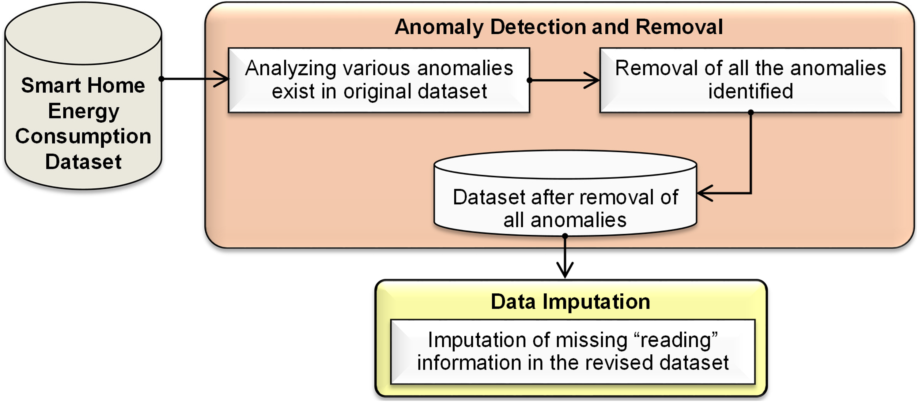
Proposed conceptual model for data anomaly detection and rectification.

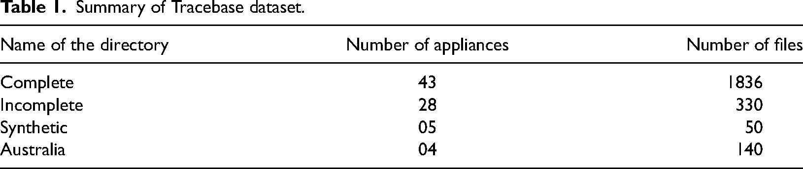
To implement the proposed process, a real-time dataset named “Tracebase dataset” of smart homes is considered (Purna Prakash and Pavan Kumar, 2022c). The summary of this dataset description is given in Table 1. Here, each file represents the data of a day that consists of timestamped energy consumption records for that day of all the appliances. For example, the directory “Complete” consists of 43 appliances and altogether produces 1836 files (represents data of 1836 days). For the analysis, this paper considers the directory “Complete.”

Table 1.

Summary of Tracebase dataset.

Name of the directory	Number of appliances	Number of files
Complete	43	1836
Incomplete	28	330
Synthetic	05	50
Australia	04	140

In the context of the considered dataset, the data preprocessing can be explained as the data preparation that includes the structuring of columns and the data type conversion. The dataset is available with a single column during the process of storing energy consumption readings. The timestamp and reading information are available in this single column of character type. The identification and handling of anomalies on this is not viable. Hence, this single-column data is split into desired multiple columns to implement the proposed method. The columns after the split are DATE, HOUR, MINUTE, SECOND, and READING. Among all these columns, except the DATE column, all the other columns are selected for implementing the proposed method as the data represents a day. The column READING is dependent on the timestamp HOUR, MINUTE, and SECOND. As these columns are required, they are selected straight away without using any feature selection method.

The detailed implementation flow of the data anomaly handling process is shown in Figure 2. Initially, it finds if there are any missing records and then looks for various anomalies namely garbage data, outliers data, and redundant data sequentially. All such identified anomalous records are to be removed. ANN models are sensitive to noise data such as outliers, redundancy, and garbage data. The noisy data may create randomness and it impact the training process. Hence, the removal of these anomalies helps the ANN model to perform the imputation of missing data effectively. This leads to the formation of the revised dataset with all missing records, which are formed by removing all anomalies. Now, for the imputation process, initially, these missing records are filled with “NA,” which indicates not available. Then, these NA data are imputed with conventional as well as the proposed ANN-based methods. As a result, a refined dataset with all clean data will be produced. The proposed method considers the missing data pattern as “missing at random (MAR)” and performs the imputation (Purna Prakash and Pavan Kumar, 2022c).

Figure 2.

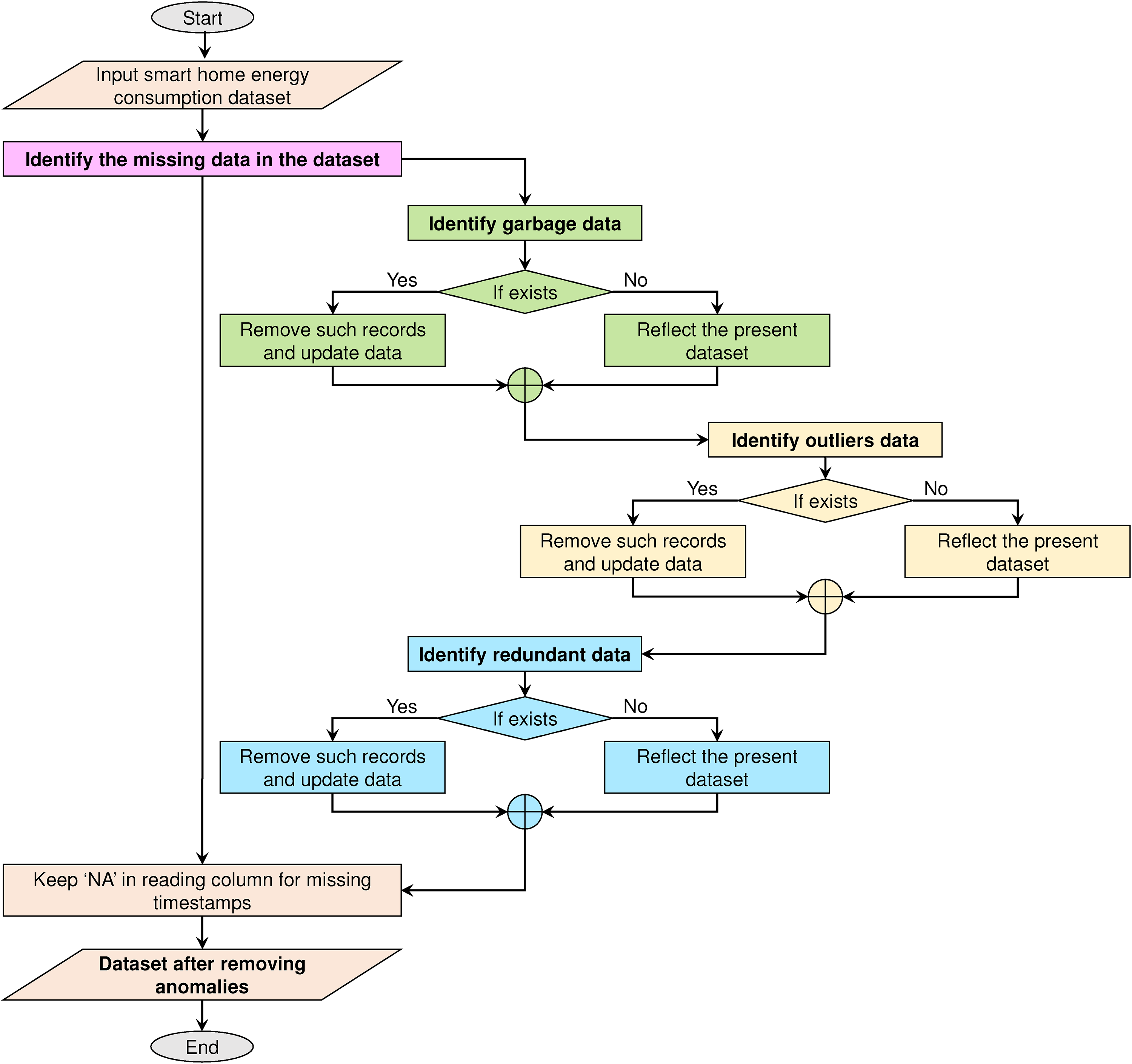
Implementation flow for identifying and removing all anomalies.

The actual expectation of the energy consumption data in the datasets is numerical data. If any character or symbol other than the numerical data that exists in the dataset is said to be garbage data. The identification of such garbage values is essential to conduct the imputation process smoothly. For the identification of the garbage data, the string pattern matching function grepl(“[[:digit:]] is implemented on each column of the data whether the data in that column is numeric or not. All the records that contain the garbage data are to be removed to effectively implement the proposed method.

Sometimes, in the energy consumption data, extreme energy consumption values may exist. It is necessary to verify whether they are useful data or outliers. During the outlier analysis, the outliers in the energy consumption data are identified based on the data distribution. Outliers mean the values that do not fall within the specified range. The existence of outliers affects the imputation process. The identification of these outliers is done by implementing the boxplot() functionality on the reading data. This approach is a standard approach for identifying the outliers by using the five-number summary. This summary includes minimum, first quartile, median, third quartile, and maximum values. From this boxplot analysis, the values that do not fall between the minimum and maximum values are said to be outliers. All the records that contain the outliers are to be removed for effective implementation of the proposed method.

Due to the congestion in the network, the energy consumption records may not be stored properly and they lead to redundancy in the dataset. Redundancy means the multiple copies of the records in the dataset. The existence of redundancy in the energy consumption data leads to ambiguity during the imputation process. Further, two types of redundant records are found in the dataset such as the records with the same timestamp and same reading information, and records with the same timestamp and different reading information.

The implementation of the proposed methodology is performed by ANNs. ANNs are computational models that mimic biological neural networks, which are the networks of interconnected neurons in the brain. ANNs are used for several applications, including pattern recognition, natural language processing, image recognition, speech recognition, and machine learning.

Feedforward neural networks are a kind of ANN that consists of multiple layers of interconnected nodes, where the output of each layer is fed as input to the next layer. The layers in the network are typically arranged in a “feedforward” manner, meaning that there are no feedback connections between layers. A typical ANN diagram is shown in Figure 3. In this, the input layer is on the left-hand side, with nodes representing the input variables. The output layer is on the right-hand side, with nodes representing the predicted outputs. The hidden layers, which are sandwiched between the input and output layers, contain nodes that perform calculations on the input data. The count of hidden layers and nodes in each layer can differ based on the complexity of the problem being addressed. In summary, an ANN diagram represents the connections and computations that occur within a neural network to process input data and generate output predictions.

Figure 3.

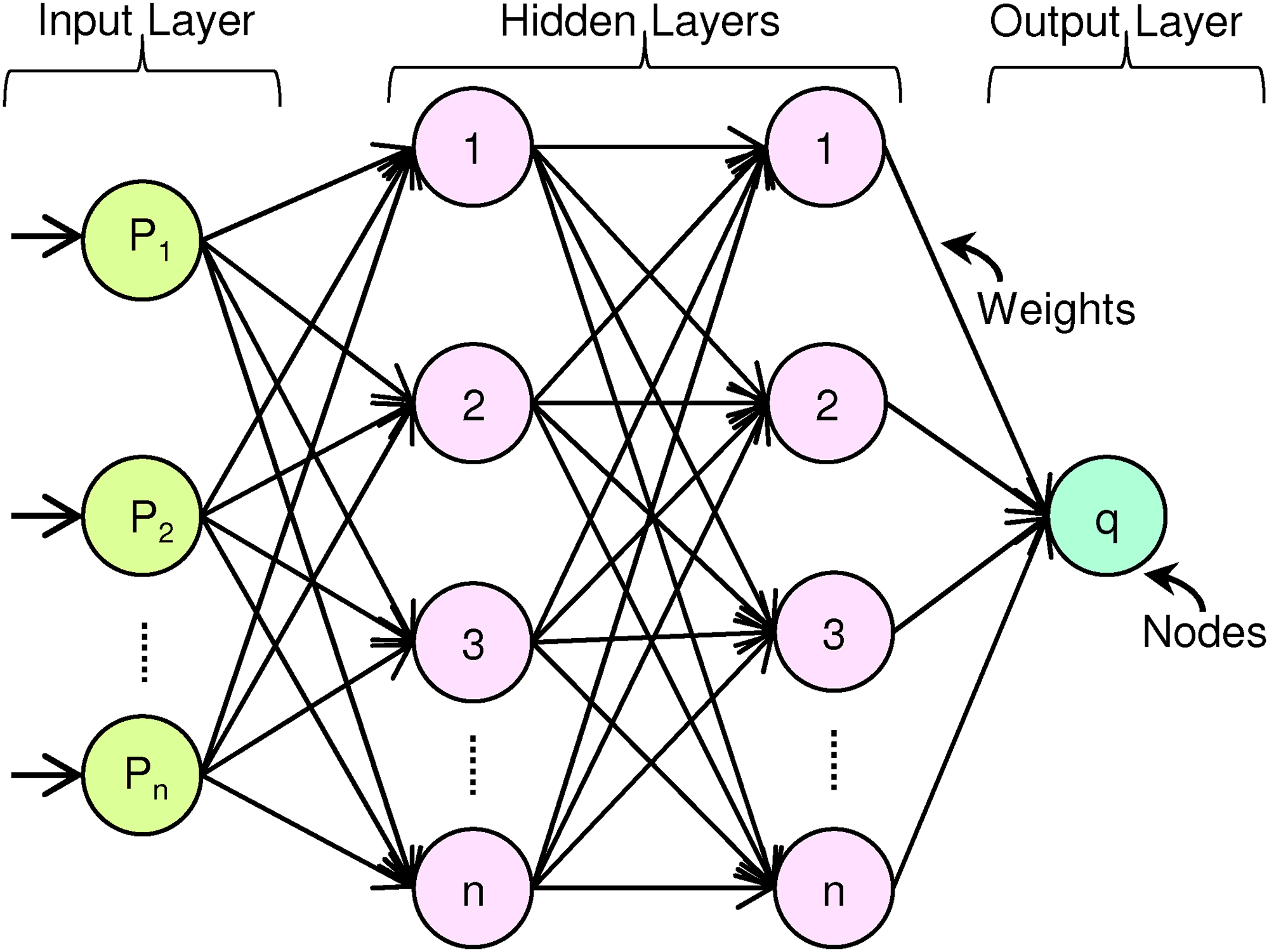
Architecture of ANN.

Artificial neural network models

This section presents ANN models namely nonlinear autoregressive neural network with external input (NARX) and nonlinear input–output neural network (NION) known as time delay network. These models are implemented by using key training algorithms viz., Levenberg–Marquardt (LM), scaled conjugate gradient backpropagation (SCG), and Bayesian regularization (BR) to impute the missing data and further improvise the imputation done by the conventional methods. The execution flow of the proposed ANN-based data imputation is shown in Figure 4.

Figure 4.

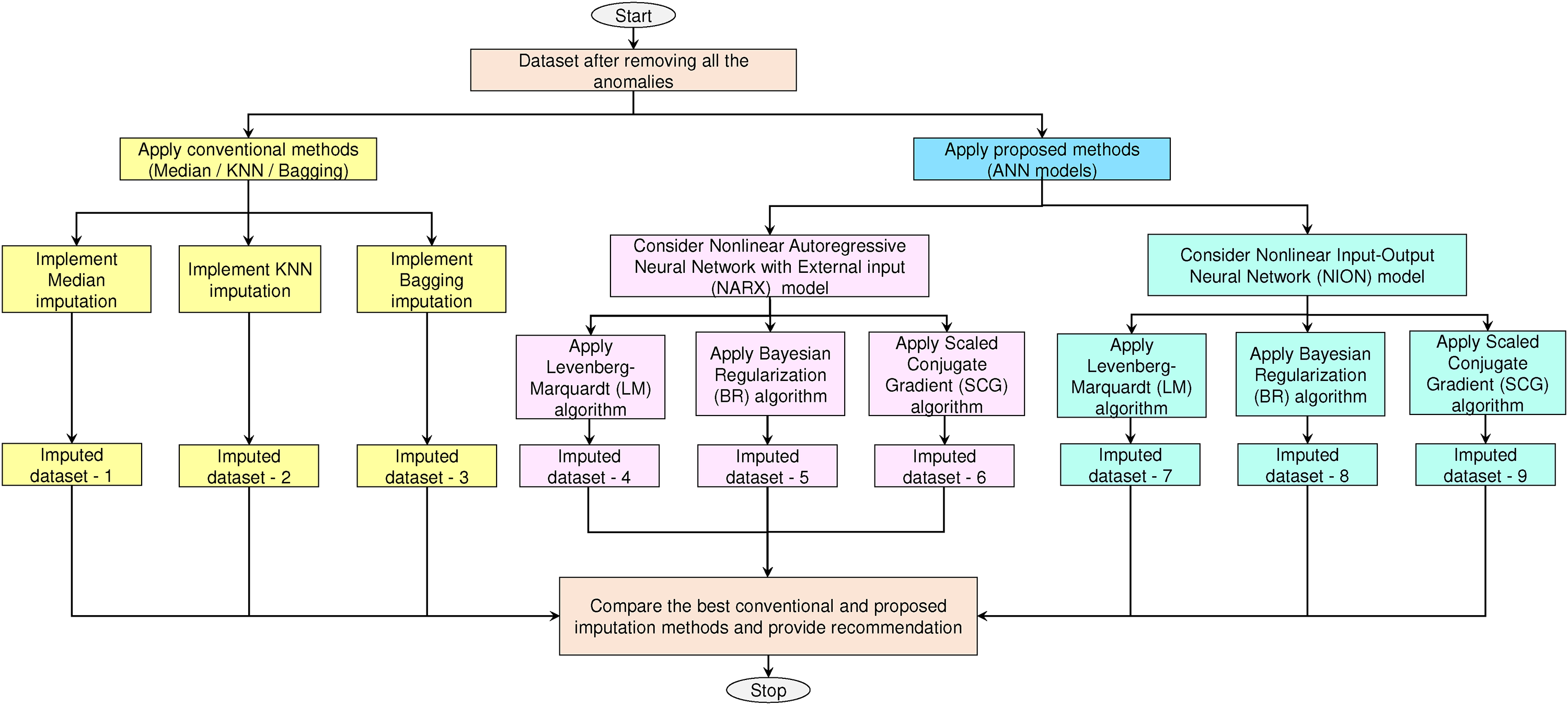
Implementation flow for data imputation.

The NARX network stands out as a neural network that is commonly used for time series prediction and control. It represents a category of feedforward neural networks that combine both feedforward and feedback connections. What sets the NARX network apart is its ability to consider past values of the time series in question, alongside external inputs that could influence it. These external inputs span a range of variables, from weather conditions to economic indicators. Within the NARX network, multiple layers of interconnected nodes, or neurons, work harmoniously to grasp intricate nonlinear relationships between inputs and outputs. Thanks to feedback connections, the network can utilize its own predictions as inputs, a feature that enables it to learn from its previous missteps and enhance its predictive accuracy over time. In broader applications, the NARX network proves itself as a potent tool for time series prediction and control, finding utility in diverse fields, including finance, economics, and engineering.

On the other hand, the NION, also known as the time delay neural network (TDNN), offers a different approach. It's an ANN type that incorporates a delay element to model dynamic systems. This network excels at mapping a set of input values to a corresponding set of output values through a nonlinear function. The temporal dynamics of a system are captured effectively by the time delay element, making the TDNN particularly suitable for modeling time series data or addressing signal processing tasks.

The network's architecture includes one or more fully connected hidden layers, with each neuron in these layers having a collection of time-delayed inputs. These inputs are weighted and summed to produce the network's output. TDNNs can undergo training through supervised learning techniques like backpropagation, which fine-tunes the network's weights and biases to minimize the error between predicted and actual output values. It's important to note that this training process can be resource-intensive and is often dependent on a substantial dataset for optimal performance.

Training algorithms

The description of the training algorithms used for the proposed ANN algorithms is given below.

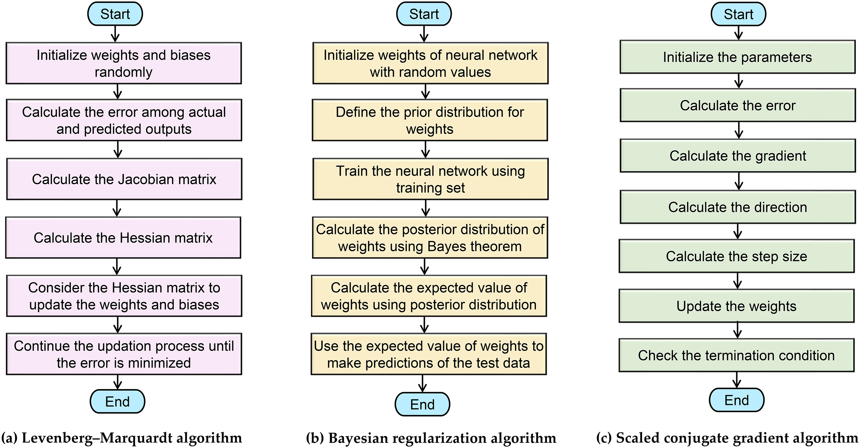
LM. It is a popular optimization algorithm used in machine learning, specifically in the training of ANNs. The LM algorithm is an iterative optimization algorithm that combines the gradient descent and Gauss-Newton methods to minimize the error function of a network. It is often used in problems where there are nonlinear relationships between inputs and outputs, making it ideal for training neural networks. The steps of the algorithm are given in Table 2 and shown in Figure 5(a). In MATLAB, the LM algorithm can be implemented using the “trainlm” function. The function takes as input the network architecture, input and output data, and many training options namely the maximum number of iterations and the minimum error tolerance. The function returns the trained network along with other information such as the final error and the number of iterations. Overall, the LM algorithm is a powerful optimization algorithm for training neural networks that can handle nonlinear relationships between inputs and outputs.

Figure 5.

Training algorithms used to train the ANN.

Table 2.

LM algorithm.

Algorithm Steps
1. The LM algorithm works by repetitively fine-tuning the weights and biases of a network to reduce the error between the predicted and actual outputs. The algorithm begins by initializing the weights and biases randomly.
2. Then, it calculates the error between the predicted and actual outputs using the current weights and biases.
3. It then calculates the Jacobian matrix, which comprises the first derivatives of the error function regarding the weights and biases.
4. It then uses the Jacobian matrix to compute the Hessian matrix, which contains the second derivatives of the error function regarding the weights and biases.
5. The Hessian matrix is considered to update the weights and biases, with the step size being determined by a damping factor that balances the gradient descent and Gauss-Newton methods.
6. It continues to iterate through these steps until the error function is minimized to a satisfactory level.

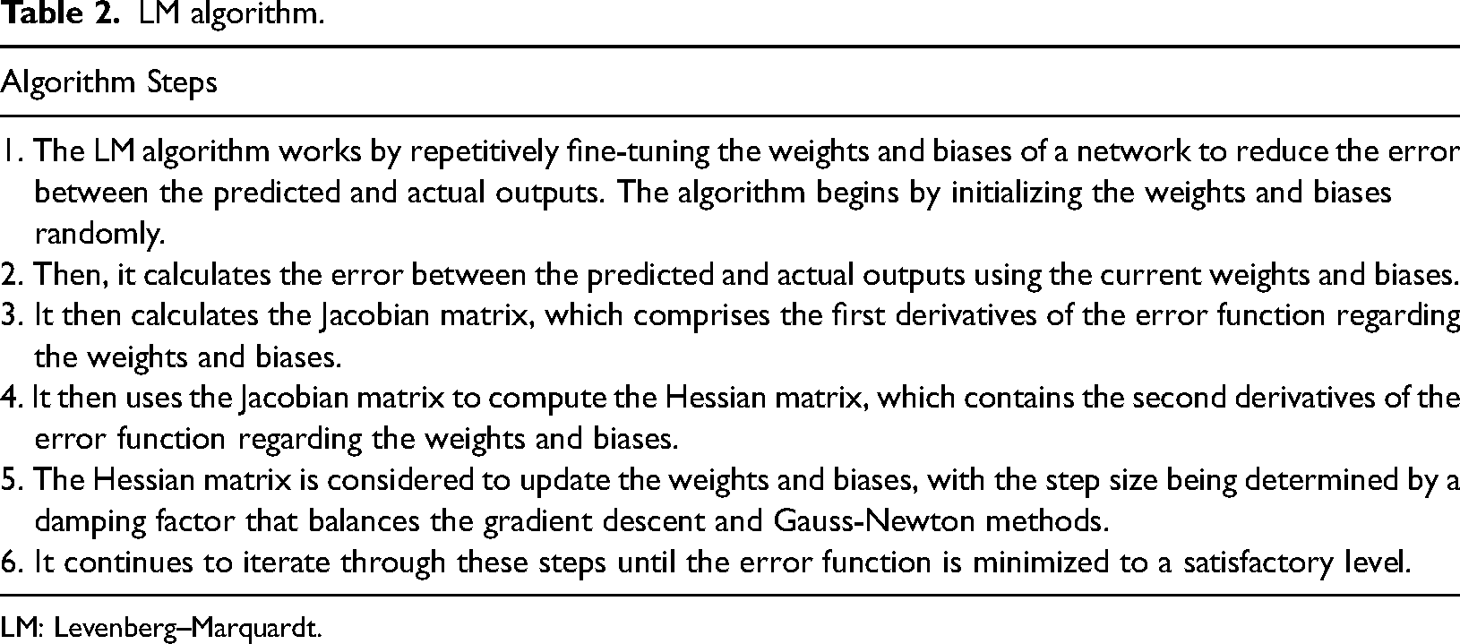
LM: Levenberg–Marquardt.

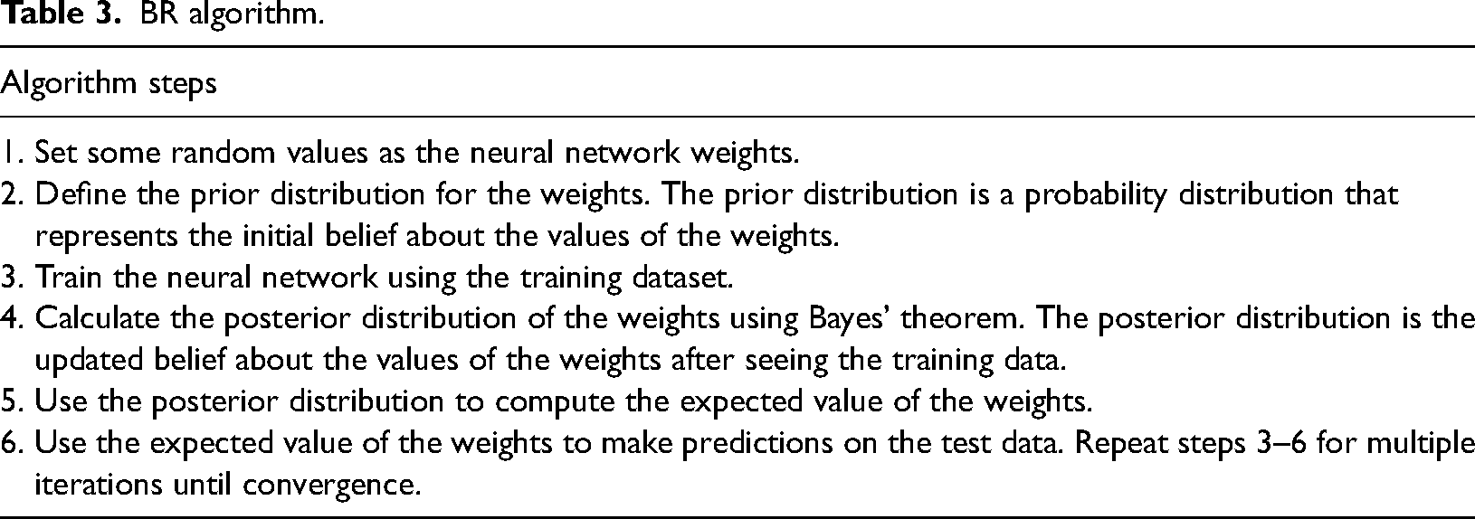
BR. It is a statistical approach used for regularizing the weights in a neural network. It provides a probabilistic interpretation of the weights and helps to prevent overfitting in the model. BR is based on Bayes’ theorem and the principle of maximum likelihood. The steps of the algorithm are given in Table 3 and shown in Figure 5(b). In MATLAB, the BR training algorithm can be implemented using the “trainbr” function in the Neural Network Toolbox. The “trainbr” function uses the BR algorithm to train a neural network.

Table 3.

BR algorithm.

Algorithm steps
1. Set some random values as the neural network weights.
2. Define the prior distribution for the weights. The prior distribution is a probability distribution that represents the initial belief about the values of the weights.
3. Train the neural network using the training dataset.
4. Calculate the posterior distribution of the weights using Bayes’ theorem. The posterior distribution is the updated belief about the values of the weights after seeing the training data.
5. Use the posterior distribution to compute the expected value of the weights.
6. Use the expected value of the weights to make predictions on the test data. Repeat steps 3–6 for multiple iterations until convergence.

SCG. It is a popular optimization algorithm used in ML and AI for training neural networks. It was first introduced by Moller in 1993 and is a variation of the conjugate gradient (CG) algorithm. The SCG algorithm uses the CG direction to calculate the minimum value of the error function and a scale factor to adjust the step size for faster convergence. The steps of the algorithm are given in Table 4 and shown in Figure 5(c). In MATLAB, the SCG training algorithm can be implemented using the “trainscg” function in the neural network toolbox. This function takes as input the neural network architecture, input/output data, and various training parameters, including learning rate, the maximum number of epochs, and convergence criteria. The function returns the trained neural network with optimized weights and biases.

Table 4.

SCG algorithm.

Algorithm steps
1. Initialize the parameters: The first step is to set the parameters namely the learning rate, maximum iterations, and minimum error tolerance.
2. Calculate the error: Calculate the error function for the given input data and the current set of weights.
3. Calculate the gradient: Calculate the gradient of the error function concerning the weights.
4. Calculate the direction: Calculate the conjugate gradient direction using the gradient and the previous direction.
5. Calculate the step size: Calculate the step size using the scale factor and the direction.
6. Update the weights: Update the weights using the step size.
7. Check the termination condition: Check if the error is below the minimum tolerance level or if the maximum number of iterations has arrived. If not, repeat the steps from step 2.

SCG: scaled conjugate gradient.

Overall, the SCG training algorithm in MATLAB provides a powerful and efficient way to optimize neural network architectures for a wide range of applications. It is known to converge faster than other optimization algorithms and is often preferred for training neural networks.

The k-fold cross-validation method with the regular folds (10 folds) is implemented on the training algorithms to quantify the uncertainty in the imputed values for the decision-making process in smart home energy management.

Results and discussion

To implement the proposed ANN models, three activation functions are used namely (a) log-sigmoid function for the input layer, (b) hyperbolic tangent function for the hidden layer, and (c) linear function for the output layer. Also, in the entire dataset, 70% of the data is considered as the training set, 15% of the data is considered as the testing set, and 15% of the data is considered as the validation set. The other specifications that are considered are Data division: Random, Layer size: 2, Time delay: 2, Predictors: Input 86400 × 3 (3 features data), and Responses: Output 86400 x (1 feature data). The summary of the implemented models, training methods, and corresponding results obtained are given in Table 5 and Table 6 respectively for the NARX model and the NION model.

Table 5.

Specifications and results of NARX model with various training algorithms.

Model and training type		Observations	Mean-square error (MSE)	Regression (R)
NARX-LM training	Training	60478	29.7023	0.9966
	Validation	12960	35.5777	0.9959
	Test	12960	28.8347	0.9967
	Epochs	16
	Elapsed time	00:00:04
NARX-BR training	Training	73438	29.8057	0.9966
	Validation	0	NaN	NaN
	Test	12960	32.6751	0.9962
	Epochs	319
	Elapsed time	00:00:21
NARX-SCG training	Training	60478	30.3632	0.9965
	Validation	12960	30.8391	0.9965
	Test	12960	33.6082	0.9962
	Epochs	97
	Elapsed time	00:00:06

NARX: nonlinear autoregressive neural network with external input; LM: Levenberg–Marquardt; SCG: scaled conjugate gradient; BR: Bayesian regularization.

Table 6.

Specifications and results of NION model with various training algorithms.

Model and training type		Observations	Mean-square error (MSE)	Regression (R)
NION-LM training	Training	60478	3932.1	0.3175
	Validation	12960	3960.4	0.3126
	Test	12960	3916	0.3217
	Epochs	42
	Elapsed time	00:00:03
NION-BR training	Training	73438	4157.5	0.2221
	Validation	0	NaN	NaN
	Test	12960	4173.1	0.2185
	Epochs	179
	Elapsed time	00:00:11
NION-SCG training	Training	60478	4312.9	0.1195
	Validation	12960	4297.6	0.1126
	Test	12960	4333.5	0.1179
	Epochs	18
	Elapsed time	00:00:01

NION: nonlinear input–output neural network; LM: Levenberg–Marquardt; SCG: scaled conjugate gradient; BR: Bayesian regularization.

The results of data imputation using the conventional imputation methods and the proposed ANN models are shown in Figure 6(a) to Figure 6(x). From Figure 6(a), it is observed that the actual reading at the timestamp 0/0/12 is 128 and the imputed reading is 128.8 by the NARX-SCG method, which is close to the actual reading when compared to other methods. Similarly, from Figure 6(b), the actual reading at the timestamp 1/35/40 is 135.18 and the imputed reading is 129.7 by the NARX-SCG method. From Figure 6(c), the actual reading at the timestamp 2/40/11 is 141 and the imputed reading is 139.6 by the NARX-SCG method. From Figure 6(d), the actual reading at the timestamp 3/14/28 is 130 and the imputed reading is 129.8 by the NARX-SCG method. From Figure 6(e), the actual reading at the timestamp 4/40/46 is 124 and the imputed reading is 124 by the median method. From Figure 6(f), the actual reading at the timestamp 5/11/31 is 135.18 and the imputed reading is 130.1 by the NARX-SCG method.

Figure 6.

Comparison of imputed and actual readings with conventional and proposed methods.

From Figure 6(g), the actual reading at the timestamp 6/28/35 is 162 and the imputed reading is 159 by the KNN method. From Figure 6(h), the actual reading at the timestamp 7/6/2 is 136 and the imputed reading is 135.75 by the NARX-SCG method. From Figure 6(i), the actual reading at the timestamp 8/16/27 is 126 and the imputed reading is 126.9 by the NARX-SCG method. From Figure 6(j), the actual reading at the timestamp 9/59/34 is 135.8 and the imputed reading is 132.7 by the NARX-SCG method. From Figure 6(k), the actual reading at the timestamp 10/27/50 is 177 and the imputed reading is 173.54 by the KNN method. From Figure 6(l), the actual reading at the timestamp 11/14/40 is 136 and the imputed reading is 135.9 by the NARX-SCG method. From Figure 6(m), the actual reading at the timestamp 12/25/33 is 124 and the imputed reading is 124 by the median method. From Figure 6(n), the actual reading at the timestamp 13/18/35 is 135.18 and the imputed reading is 130.6 by the NARX-SCG method. From Figure 6(o), the actual reading at the timestamp 14/24/52 is 154 and the imputed reading is 155.56 by the KNN method. From Figure 6(p), the actual reading at the timestamp 15/7/3 is 132 and the imputed reading is 131.74 by the NARX-SCG method.

From Figure 6(q), the actual reading at the timestamp 16/24/18 is 124 and the imputed reading is 124 by the median method. From Figure 6(r), the actual reading at the timestamp 17/59/6 is 173 and the imputed reading is 175.7 by the KNN method. From Figure 6(s), the actual reading at the timestamp 18/17/56 is 149 and the imputed reading is 149 by the KNN method. From Figure 6(t), the actual reading at the timestamp 19/44/2 is 128 and the imputed reading is 128.2 by the NARX-SCG method. From Figure 6(u), the actual reading at the timestamp 20/2/23 is 126 and the imputed reading is 125.8 by the NARX-SCG method. From Figure 6(v), the actual reading at the timestamp 21/48/40 is 171 and the imputed reading is 171.22 by the KNN method. From Figure 6(w), the actual reading at the timestamp 22/2/49 is 154 and the imputed reading is 151.25 by the KNN method. From Figure 6(x), the actual reading at the timestamp 23/8/3 is 130 and the imputed reading is 130.4 by the NARX-SCG method.

From these results, it is observed that the performance of NARX-SCG is superior to all the other imputation methods. Here, the average reading value (135.18) in the READING column is calculated after ignoring the anomalous readings. This average value is considered a base to observe the effectiveness of the imputation methods where the reading value is anomalous. The comparison of proposed ANN models with conventional methods is given in Table 7.

Table 7.

Comparison of proposed ANN models with conventional methods for data imputation.

Hour	Timestamp (HMS)	Actual reading	Conventional methods			Proposed ANN models
Hour	Timestamp (HMS)	Actual reading	Median	KNN	Bagging	NARX-LM	NARX-BR	NARX-SCG	NION -LM	NION -BR	NION-SCG
0	0 0 12	128	124	126	125.69	161.1	155.1	128.8	70.93	67.86	78.73
1	1 35 40	0 (anomaly)	124	0	0.00	158.8	0.2721	129.7	70.93	80.34	68.49
2	2 40 11	141	124	142	135.09	157.7	0.2753	139.6	70.93	80.71	65.35
3	3 14 28	130	124	129.65	135.09	159.8	150	129.8	70.93	67.86	78.26
4	4 40 46	124	124	122.97	123.96	158	0.09001	414.2	70.93	80.71	68.83
5	5 11 31	0 (anomaly)	124	0	0	158.4	0.5614	130.1	70.93	80.71	77.11
6	6 28 35	162	124	159	127.11	158.4	0.5614	130.1	70.93	80.71	77.11
7	7 6 2	136	124	135.23	130.38	161.3	156	135.75	70.93	67.86	79.09
8	8 16 27	126	124	123	130.38	158.9	151.2	126.9	70.93	79.16	78.9
9	9 59 34	0 (anomaly)	124	0	0.00	158.3	0.4697	132.7	70.93	80.71	54.9
10	10 27 50	177	124	173.54	142.59	158.1	0.5114	130.4	70.93	80.71	78.54
11	11 14 40	136	124	137	137.03	158.8	151.9	135.9	69.81	80.71	79.26
12	12 25 33	124	124	126	125.14	157.6	147.7	130.7	70.93	80.71	79.23
13	13 18 35	0 (anomaly)	124	0	0.02	158.1	151.6	130.6	69.81	80.71	79.52
14	14 24 52	154	124	155.56	140.10	0.2185	146.3	130.7	69.81	80.71	79.54
15	15 7 3	132	124	133.08	134.69	0.2644	157.8	131.74	69.81	80.61	79.91
16	16 24 18	124	124	125.01	126.16	0.0088	152.1	131.3	69.81	80.71	80.36
17	17 59 6	173	124	175.7	161.80	−0.645	−0.3879	414.3	70.93	80.71	77.19
18	18 17 56	149	124	149	137.02	0.207	151.9	130.9	69.81	80.71	80.26
19	19 44 2	128	124	126	137.02	−0.488	−0.245	128.2	69.81	80.71	82.7
20	20 2 23	126	124	124.39	125.51	0.1692	160.1	125.8	69.81	80.71	80.82
21	21 48 40	171	124	171.22	165.55	−0.472	−0.2403	414.3	135.8	80.71	83.18
22	22 2 49	154	124	151.25	131.8	0.2832	158	131	135.8	80.71	80.75
23	23 8 3	130	124	128	131.8	−0.036	159.5	130.4	135.8	80.71	82.37

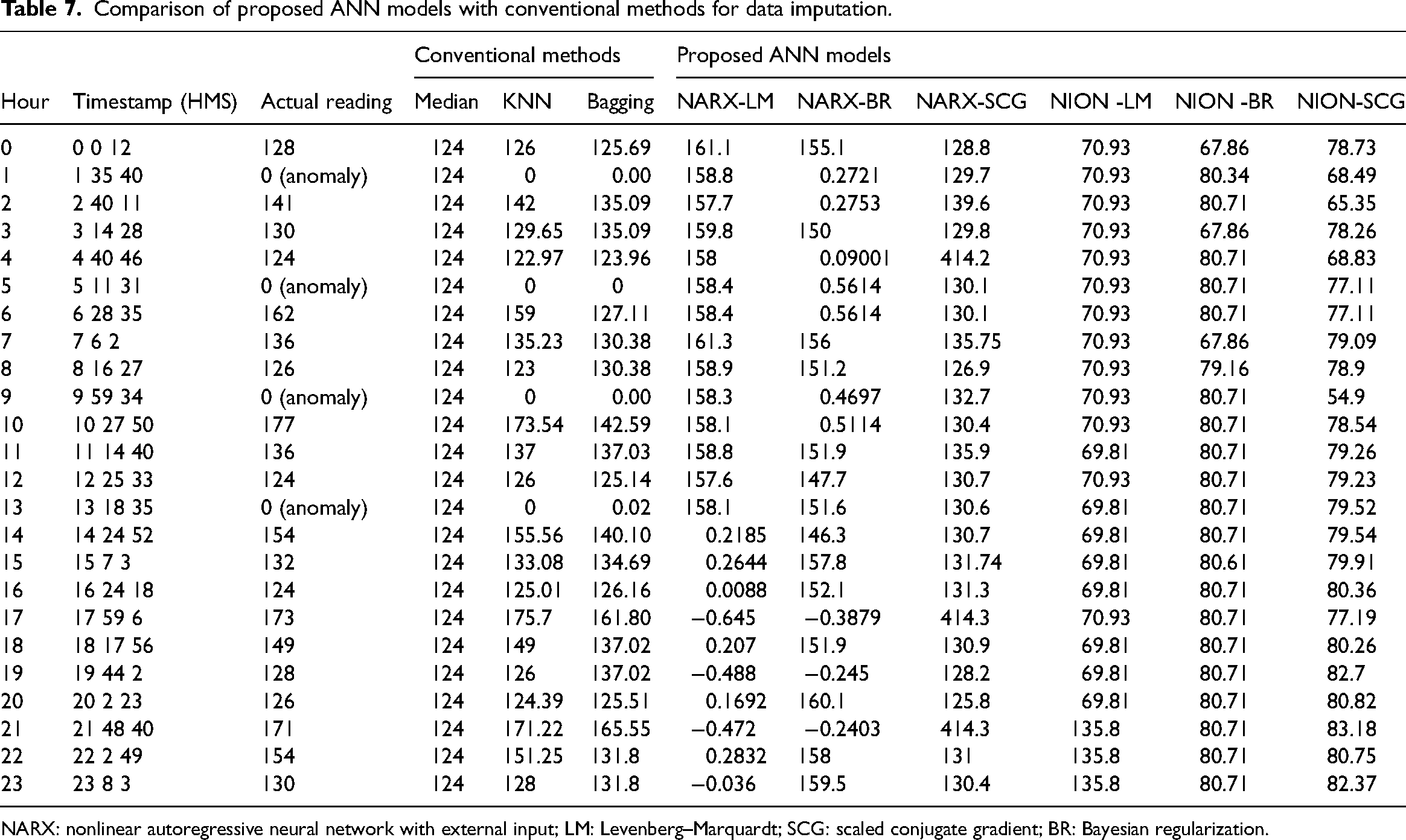
NARX: nonlinear autoregressive neural network with external input; LM: Levenberg–Marquardt; SCG: scaled conjugate gradient; BR: Bayesian regularization.

Conclusions

As smart home technologies continue to evolve and play an increasingly vital role in the broader context of environmental sustainability, the proposed ANN-based data imputation method provides a robust foundation for ensuring the integrity of energy consumption data. It empowers decision-makers with more precise insights, facilitating informed choices to optimize energy usage and reduce environmental impact. In essence, this research not only contributes to the advancement of smart home technologies but also aligns with the global agenda for sustainable living. It underscores the importance of data quality in achieving energy efficiency and highlights the potential of ANN-based data imputation as a transformative tool in the pursuit of a greener, more sustainable future. The salient observations are given as follows.

▪ All the probable anomalies are effectively detected and eliminated from the dataset. The original dataset consists of 155,374 records, whereas the refined dataset consists of 86,400 records after removing anomalies, which is the desired count of records as per the description of the dataset.

▪ Among these 86,400 records, it is found that there are 13,803 records are missed. All these missed data have been effectively imputed by using both conventional and proposed imputation methods. Even though the conventional imputation methods perform well in normal cases, they are failing while recalculating the readings in the case of anomalous readings. However, the proposed ANN models can recalculate the approximate reading values which is the advantage of implementing the ANN models over conventional imputation methods.

▪ Further, it is evident that the NARX-SCG ANN model has achieved superior performance over the other types of ANN models and imputed the data accordingly.

The ANN models proposed in this paper demonstrated an approach that not only imputes missing values but also identifies and corrects anomalies within energy consumption datasets. The findings indicate that this approach surpasses traditional imputation techniques in terms of accuracy and robustness, effectively enhancing the quality and completeness of the data. In conclusion, this research has illuminated the potential of ANN-based data imputation as a powerful tool for addressing the challenges posed by missing and anomalous data in the context of smart home electrical energy consumption monitoring.

Scope, merits, and limitations

The data are trained by all the proposed ANN models and the training algorithms. Out of them the NARX model with the training algorithm SCG algorithm has achieved the superior performance. The NARX-SCG model has successfully imputed the missing values in the smart home energy consumption data. It is applied to the numerical data of energy consumption and its performance is good. Thus, the scope of the proposed methods is limited to numerical data. So, it is expected that these methods achieve similar performance for any other applications with similar type of data. However, there is a risk of overfitting, and it can be handled by setting the number of epochs during the training of the data. However, too many epochs lead to overfitting and less number of epochs lead to underfitting. Thus, the number of epochs for the training can be decided based on the size of the data.

Specific merits of the proposed models in this paper are summarized as follows.

▪ Computational Efficiency: The trade-off between computational resources and imputation accuracy in ANN-based data imputation depends on the type and complexity of the application data. In the considered smart home application, the energy consumption data is a simple numerical type data, thereby less complex models are sufficient to handle such datasets. Besides, the neural networks integrally offer parallelism. This characteristic allows the algorithms to perform the training effectively even on large volumes of data. The proposed method takes advantage of parallelism and supports the training and simulation without any computational hurdles. Hence, the computational resources do not affect the smart home data and the computational cost is taken care of by the parallelism in neural networks.

▪ Scalability and Robustness: The proposed neural network models allow parallel and distributed computing. These features allow the speeding up of the training and simulation of the neural networks and deal with large volumes of data even that contain varying ratios of anomalous data. The intermediate results are automatically saved at checkpoints when the neural network training runs long period. This ensures the recovery of the training in case of failures. Further, the management of temporary storage for the process will increase the performance of the proposed method. All these allow the proposed method to scale with different sizes and varying numbers of appliances and sensors.

Footnotes

Author contributions

KPP and YVPK, designed the study; KR, collected the data; MA and BK, performed the analysis and interpreted the results; KPP and GPR, drafted the manuscript. All authors reviewed and approved the final version of the manuscript.

Declaration of conflicting interests

The author(s) declared no potential conflicts of interest with respect to the research, authorship, and/or publication of this article.

Funding

The author(s) received no financial support for the research, authorship, and/or publication of this article.

Data availability statement

Not applicable.

ORCID iD

Yellapragada Venkata Pavan Kumar

References

Aguilar

Garces-Jimenez

R-Moreno

, et al. (2021) A systematic literature review on the use of artificial intelligence in energy self-management in smart buildings. Renewable and Sustainable Energy Reviews 151: 111530.

Ahmed

Abdulrazak

Blanchet

, et al. (2022) Long gaps missing IoT sensors time series data imputation: A Bayesian Gaussian approach. IEEE Access 10: 116107–116119.

Attar

Schirle

Hofmann

(2022) Noise added on interpolation as a simple novel method for imputing missing data from household’s electricity consumption. Procedia Computer Science 207: 2253–2262.

Borges

Kamara-Esteban

Castillo-Calzadilla

, et al. (2020) Enhancing the missing data imputation of primary substation load demand records. Sustainable Energy, Grids and Networks 23: 100369.

Fazakis

Kostopoulos

Kotsiantis

, et al. (2020) Iterative robust semi-supervised missing data imputation. IEEE Access 8: 90555–90569.

Himeur

Ghanem

Alsalemi

, et al. (2021) Artificial intelligence based anomaly detection of energy consumption in buildings: A review, current trends and new perspectives. Applied Energy 287: 116601.

Jeong

Park

(2021) Missing data imputation using mixture factor analysis for building electric load data. Applied Energy 304: 117655.

Jiang

Tian

(2021) A graph-based approach for missing sensor data imputation. IEEE Sensors Journal 21(20): 23133–23144.

Jurado

Nebot

Mugica

, et al. (2017) Fuzzy inductive reasoning forecasting strategies able to cope with missing data: A smart grid application. Applied Soft Computing 51: 225–238.

10.

Kim

Chung

(2020) Multi-modal stacked denoising autoencoder for handling missing data in healthcare big data. IEEE Access 8: 104933–104943.

11.

Lai

Zhang

Liu

(2020) Takagi-Sugeno modeling of incomplete data for missing value imputation with the use of alternate learning. IEEE Access 8: 83633–83644.

12.

Lee

Han

Choi

(2021) MPdist-based missing data imputation for supporting big data analyses in IoT-based applications. Future Generation Computer Systems 125: 421–432.

13.

Leiria

Johra

Marszal-Pomianowska

, et al. (2021) Using data from smart energy meters to gain knowledge about households connected to the district heating network: A Danish case. Smart Energy 3: 100035.

14.

Liao

Bak-Jensen

Radhakrishna Pillai

, et al. (2022) Data-driven missing data imputation for wind farms using context encoder. Journal of Modern Power Systems and Clean Energy 10(4): 964–976.

15.

Liu

Zhang

(2021) A two-stage deep autoencoder-based missing data imputation method for wind farm SCADA data. IEEE Sensors Journal 21(9): 10933–10945.

16.

Liu

Dillon

, et al. (2020) Missing value imputation for industrial IoT sensor data with large gaps. IEEE Internet of Things Journal 7(8): 6855–6867.

17.

Mei

(2018) An imputation method for missing data based on an extreme learning machine auto-encoder. IEEE Access 6: 52930–52935.

18.

Cheng

JCP

Jiang

, et al. (2020) A bi-directional missing data imputation scheme based on LSTM and transfer learning for building energy data. Energy and Buildings 216: 109941.

19.

McCombe

Liu

Ding

, et al. (2022) Practical strategies for extreme missing data imputation in dementia diagnosis. IEEE Journal of Biomedical and Health Informatics 26(2): 818–827.

20.

Miao

Chen

, et al. (2023) An experimental survey of missing data imputation algorithms. IEEE Transactions on Knowledge and Data Engineering 35(7): 6630–6650.

21.

Psychogyios

Ilias

Ntanos

, et al. (2023) Missing value imputation methods for electronic health records. IEEE Access 11: 21562–21574.

22.

Purna Prakash

Pavan Kumar

(2021) Simple and effective descriptive analysis of missing data anomalies in smart home energy consumption readings. Journal of Energy Systems 5(3): 199–220.

23.

Purna Prakash

Pavan Kumar

(2022a) Analytical approach to exploring the missing data behavior in smart home energy consumption dataset. Journal of Renewable Energy and Environment 9(2): 37–48.

24.

Purna Prakash

Pavan Kumar

(2022b) Exploration of anomalous tracing of records in smart home energy consumption dataset. ECS Transactions 107(1): 18271–18280.

25.

Purna Prakash

Pavan Kumar

(2022c) Systematic statistical analysis to ascertain the missing data patterns in energy consumption data of smart homes. International Journal of Renewable Energy Research 12(3): 1560–1573.

26.

Purna Prakash

Pavan Kumar

Moganti

GLK

, et al. (2022d) Machine learning-based ensemble classifiers for anomaly handling in smart home energy consumption data. Sensors 22(23): 9323.

27.

Purna Prakash

Pavan Kumar

Reddy

, et al. (2022e) A comprehensive analytical exploration and customer behaviour analysis of smart home energy consumption data with a practical case study. Energy Reports 8: 9081–9093.

28.

Razavi-Far

Farajzadeh-Zanjani

Saif

, et al. (2020) Correlation clustering imputation for diagnosing attacks and faults with missing power grid data. IEEE Transactions on Smart Grid 11(2): 1453–1464.

29.

Schreiber

Sausen

De Campos

, et al. (2023) Data imputation techniques applied to the smart grids environment. IEEE Access 11: 31931–31940.

30.

Shi

, et al. (2021) Nonlinear compensation algorithm for multidimensional temporal data: A missing value imputation for the power grid applications. Knowledge-Based Systems 215: 106743.

31.

Venugopalan

Chanani

Maher

, et al. (2019) Novel data imputation for multiple types of missing data in intensive care units. IEEE Journal of Biomedical and Health Informatics 23(3): 1243–1250.

32.

Wang

Tsai

Lin

(2021) Towards missing electric power data imputation for energy management systems. Expert Systems with Applications 174: 114743.

33.

Weber

Turowski

Cakmak

, et al. (2021) Data-driven copy-paste imputation for energy time series. IEEE Transactions on Smart Grid 12(6): 5409–5419.

34.

Hamshaw

Yang

, et al. (2022) Data imputation for multivariate time series sensor data with large gaps of missing data. IEEE Sensors Journal 22(11): 10671–10683.

35.

Yao

Zhao

(2022) FIGAN: A missing industrial data imputation method customized for soft sensor application. IEEE Transactions on Automation Science and Engineering 19(4): 3712–3722.

Artificial neural network-based data imputation for handling anomalous energy consumption readings in smart homes

Abstract

Keywords

Introduction

Methodology

Artificial neural network models

Training algorithms

Results and discussion

Conclusions

Scope, merits, and limitations

Footnotes

Author contributions

Declaration of conflicting interests

Funding

Data availability statement

ORCID iD

References