Sage Journals: Discover world-class research

Abstract

In this article, a modified immersed boundary method (IBM) with a ghost-cells strategy is introduced to study a kind of vertical-axis wind turbine (VAWT). In order to improve the accuracy of the numerical calculation and enhance its adaptability, some treatments on the IBM for the VAWT especially are carried out. The method is testified by the numerical simulation of an Eppler387 airfoil. With the help of the method, some flowing characteristics of the wind turbine have been thoroughly observed and understood. Furthermore, the effects of blade shape, tip vortex and secondary flowing on the turbine performance are discussed in detail based on the numerical results.

Keywords

Immersed boundary method vertical-axis wind turbine tip vortex secondary flowing airfoil

Introduction

Compared with fossil fuel energy, wind energy is considered as a kind of green energy and gradually attracts more interest in the world. The study of wind energy absorbers also becomes more and more popular recently. Wind turbine is one of the most important equipments in an absorber unit. In general, wind turbine can be divided into two different types based on its rotational axis, such as horizontal-axis wind turbines (HAWTs) and vertical-axis wind turbines (VAWTs). Indeed, these two types of wind turbines both have their own advantages and applications. Compared with the HAWT, the VAWT has advantages, such as lower sound emission and high adaptability to yaw (Ferreira et al., 2006).

Numerical simulation is one of the most important methods to study wind turbine performance. It was due to the limitation of computation resources that the initial research mainly relied on some simplified mathematic methods. These methods were related to some models, such as stream-tube model and free vortex model. Templin (1974) innovatively put forward momentum model for the wind turbine performance simulation, which was called single stream-tube model. In this model, wind blades were simplified as one driven disk, and power output of a wind turbine was estimated by the momentum differences between upwind and downwind regions. In order to consider the effect of local Reynolds number on the airfoil performance, Strickland (1975) introduced a multiple stream-tube model in 1975. He discretized the computational region by a series of stream tubes rather than a single stream tube. In order to improve the precision of the model, Nguyen (1979) proposed a free vortex model to predict the wind turbine performance. In his model, blades were described by a vortex sheet so that some detailed flowing features were also observed thereupon, such as interactions between blades and blades, blades and wake and so on.

Though the turbine performance could be studied with the help of the simplified models, some important aerodynamic characteristics were still undiscovered, especially for the cases with larger tip speed ratio. So, advanced computational fluid dynamics (CFD) technology had been gradually applied to the study of the VAWT. Based on a 2D model, Wolfe and Ochs (1997) studied the aerodynamic performance of a kind of wind turbine airfoil by CFD simulation with k-ε turbulence model. The results showed that k-ε turbulence model was not sufficient to accurately describe flow separation with large attack angle. Chen and Lian (2015) also conducted research on 2D model of a kind of H-rotor VAWT by unsteady numerical simulation. The effects of the blade solidity and thickness on aerodynamic performance were studied in their paper. 2D large eddy simulation (LES) was applied to the VAWT by Lida et al. (2007). It was found that under low tip speed ratio conditions, power output obtained from 2D LES was obviously different from that based on the momentum model though the method of 2D LES seems not to be reasonable. In Das et al. (2021), the performance analysis of two straight-bladed Darrieus VAWT equipped with symmetrical (NACA 0018) & cambered airfoils (S1210) were studied in dynamic stall region. A comparative 2D numerical simulation had been conducted to forecast the performance of wind turbine with two different types of blades. With the rapid progress of CFD technology, it was possible to thoroughly estimate the performance of the VAWT by a 3D model. Howell et al. (2010) conducted U-RANS simulation with help of a 3D model of a small VAWT based on RNG k-ε turbulence model. In his study, compared with 2D simulation, 3D effects on performance could be clearly observed. Ye et al. (2023) adopted RANS equations with the k − ω SST turbulence model to study the wake characteristics of a model-scale HAWT. A thorough verification and validation study was performed to quantify the numerical uncertainties in the CFD results. Pedram et al. (2023) used Fluent software to explore the performance of the Darrius type wind turbine at blade tip speeds around 1. Indhumathy and Mahalakshmi (2022) investigated the performance of a new VAWT with non-cylindrical helical turbine blades for an unsteady gusty wind prevailing in urban and suburban environments. In his work, three-dimensional CFD analysis with dynamic mesh had been carried out for two gust velocities of 0.6 and 2 m/s with a mean free stream velocity of 4 m/s. Aerodynamic performance analysis of all airfoils with the ANSYS Fluent software was carried out by Mohd et al. (2023). In his paper, the performance of NACA 0012 and NACA4412 was compared with a VAWT model. Cameron et al. (2023) adopted 3D CFD simulations in ANSYS Fluent to analyze the performance of a small-scale hybrid VAWT. The numerical results had similar trends to the data from experiments, but there was still obvious difference between results from the simulations and experiments.

All CFD simulations mentioned above were based on the body-fitted grid. In general, the VAWT is a kind of rotating machine so that the computational region is usually divided into two parts, such as the stationary part and the rotating part. In order to deal with data transferring between two regions, an advanced technology, sliding mesh technology, must be used in the calculation. Furthermore, the relative position of these two regions must be recognized on every time step in the unsteady simulation. Thus, it would take too much time on the mesh generation and data transferring, especially for some VAWTs which had complex geometrical structure. On the other hand, part of unsteady information could be lost during the process of data transferring between the stationary and the rotating cells.

An alternative method, named as immersed boundary method (IBM), is adopted in this paper to solve the above-mentioned issues on the VAWT's numerical simulation. the IBMs can be categorized into two types based on how to deal with the forcing term, such as the continuous forcing approach and the discrete forcing approach. IBM was introduced by Peskin (1977), and it was first applied to the study of flow pattern of heart blood. The effects of an immersed boundary on flow pattern were considered by adding a continuous forcing term to Naiver–Stokes equation before they were discretized. Another type of IBM was proposed by Fadlun et al. (2000). In his method, the immersed boundary condition was satisfied with the aid of a discrete force, which could be derived by boundary conditions and interpolation schemes. Due to its convenience during the mesh generating process, the IBM was gradually applied to the study of the flow filed. A sharp interface IBM for subsonic compressible viscous flow was introduced by Ghias et al. (2007), and it was applied for the simulation of 3D cylinder and Eppler211 airfoil. However, because curvilinear mesh scheme was used in his method, the benefit from the mesh generation by the IBM was weakened somewhat. Castiglioni et al. (2014) proposed an IBM-LES method for compressible flow with infinite volume discretization. In his method, non-uniform Cartesian mesh was applied to capture the flow separation-flowing point by the adjusting of the mesh density in some regions. Tay et al. (2015) proposed a block-based non-uniform mesh generation method for the application of the IBM to the cases with the moving solid boundary. In his work, he compared the simulation results obtained by several kinds of numerical methods, such as continuous forcing IBM, discrete forcing IBM and some body-fitted methods. The results showed that even though IBM cost more computational resources than other body-fitted methods, the aerodynamic performance of a single flapping wing predicted by IBM was matched with experimental data better. Barba and Stoesser (2017) applied the IBM to 3D incompressible flowing simulation to study a real hydrokinetic turbine. Liu et al. (2018) adopted a kind of ghost-cell IBM to develop a coupled aero-elasticity scheme, by which the blade vibration of a stream turbine triggered by the unsteady aerodynamic force was analyzed based on a full-annulus passages model. Gaikwad et al. (2021) described on how to adopt a ghost-point IBM in a finite-difference large-eddy code to simulate flow in atmospheric boundary layer over hills or cliffs. The roles of railings in the determining of the aerodynamic characteristics of bridge girders were investigated numerically by Wang and Cao (2022). The direct forcing IBM was utilized to model the railings while the bridge girder was modeled by body-fitted mesh system. Wang et al. (2022) presented a hybrid immersed-boundary/body-fitted-grid method to simulate flows with immersed moving boundaries. The wall-modeled large eddy simulation was employed for the simulating of turbulence. Numerical experiment was performed for the pulsatile flow through a curved, pipe bend. The predicted results showed good agreements with the published experimental data and numerical result. Huang and Carlos (2022) presented a new IBM for the simulation of compressible viscous flow. The method was based on the singular source approach where the immersed boundary added surface singularities to the governing equations. A fully three-dimensional fluid-structure interaction simulation of a subsonic parachute was showcased to demonstrate applicability to a real problem. The motivation of Xu and Huang (2023) work was to evaluate local surface stresses and hydrodynamic forces acting on a stationary or moving body by the using of a diffuse interface IBM. In his study, the concept of the immersed boundary layer was brought forward, and the dynamic effects of particle advection and collision were coupled and evaluated within a numerical time step. By the using of the open-source toolbox FOAM-Extend version 4.0 and 4.1, Giahi and Bergstrom (2023) studied a kind of IBM, which was a kind of cut-cell finite volume immersed boundary technique. By integrating the Lagrangian equations of motion with the immersed boundary, the solver was capable of simulating fluid–particle interactions.

Based on the above introduction, it is demonstrated that some detail results could be reserved without additional strategy for data exchanging between the stationery and the rotating cells by the using of the IBM, especially for the unsteady calculation. Thus, it is believed that the IBM is beneficial to the numerical simulation of the VAWT though few published materials were focused on the application of the method to this field currently.

In view of this, the efforts in this paper are mainly focused on the describing of the salient of a kind of numerical method for the performance analysis of the VAWT. In the method, a kind of ghost-cell discrete forcing IBM is combined with some special treatments to deal with the solid boundary of the rotational machine. The accuracy of the method is validated by the comparison of the simulation results of Eppler387 with the published experimental data. By the means of the IBM, some typical aerodynamic characteristics of the VAWT is analyzed and discussed in the followed words.

Numerical method

Governing equations

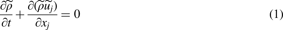
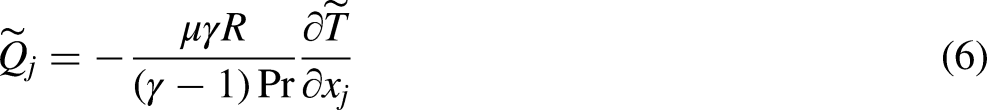
The unsteady and compressible N-S equations can be transferred into the following formula by the processing of a low-pass filter function, which is referred to LES scheme.

\frac{\partial \tilde{ρ}}{\partial t} + \frac{\partial (\tilde{ρ} \tilde{u_{j}})}{\partial x_{j}} = 0

(1)

\frac{\partial (\tilde{ρ} \tilde{u_{i}})}{\partial t} + \frac{\partial (\tilde{ρ} \tilde{u_{i}} \tilde{u_{j}})}{\partial x_{j}} + \frac{\partial \tilde{p} δ_{i k}}{\partial x_{i}} - \frac{\partial \tilde{σ_{i j}}}{\partial x_{j}} - \frac{\partial \tilde{τ_{i j}}}{\partial x_{j}} = 0

(2)

\frac{\partial \tilde{E_{t}}}{\partial t} + \frac{\partial (\tilde{E_{t}} + \tilde{p}) \tilde{u_{j}}}{\partial x_{j}} - \frac{\partial \tilde{σ_{i j}} \tilde{u_{i}}}{\partial x_{j}} + \frac{\partial {\tilde{Q}}_{j}}{\partial x_{j}} + \tilde{u_{i}} \frac{\partial {\tilde{τ}}_{i j}}{\partial x_{j}} = 0

(3)

where

\tilde{E_{t}}

is total energy.

\tilde{σ_{i j}}

and

\tilde{τ_{i j}}

are stress tensors, which can be expressed by the following equations.

{\tilde{σ}}_{i j} = μ [(\frac{\partial \tilde{u_{i}}}{\partial x_{j}} + \frac{\partial \tilde{u_{j}}}{\partial x_{i}}) - \frac{2}{3} δ_{i j} \frac{\partial \tilde{u_{k}}}{\partial x_{k}}]

(4)

{\tilde{τ}}_{i j} = μ_{S G S} [(\frac{\partial \tilde{u_{i}}}{\partial x_{j}} + \frac{\partial \tilde{u_{j}}}{\partial x_{i}}) - \frac{2}{3} δ_{i j} \frac{\partial \tilde{u_{k}}}{\partial x_{k}}]

(5)

where

μ_{S G S}

is subgrid viscosity. And, heat flux can be calculated by equation (6).

{\tilde{Q}}_{j} = - \frac{μ γ R}{(γ - 1) Pr} \frac{\partial \tilde{T}}{\partial x_{j}}

(6)

It is for the convenience that the superscript, ^~ is omitted in the following text.

Immersed boundary method

Points identification

In this paper, the discrete forcing IBM is used rather than continuous forcing IBM, since the discrete forcing IBM can maintain a sharp immersed boundary and ensure the boundary conditions furthest in the dealing with the moving solid boundary. In this discrete forcing IBM, all mesh points are classified into three types based on its affiliated region and distance to solid wall, such as inner solid points, near-wall fluid points and fluid points, marked by point1, 2, 3 in Figure 1, respectively.

Figure 1.

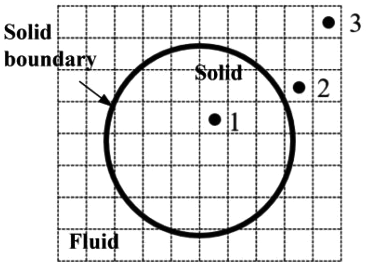
Classification of mesh points in the IBM.

The estimating of the distance from a mesh point to the solid boundary is very important to the IBM and must be calculated carefully. The distance calculation can be divided into two steps. The first step is the estimation of normal direction. The mesh points on the blade surface are taken as Maker Points (MP). The blade surface are marked by a series of MPs, which can be tracked by a array, [I, J]. In this array, I is along span-wise direction and J along airfoil chord direction. 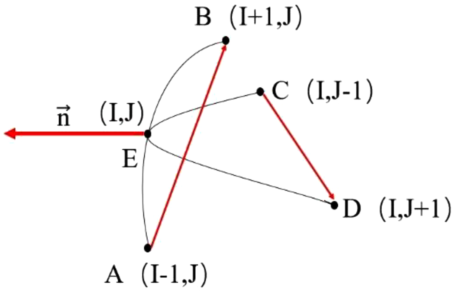The calculation of normal direction $\vec{n}$ to the blade surface at a MP, point E, is achieved by a cross product of $\vec{A B}$ and $\vec{C D}$ . Point A, B, C and D are all MPs close to point E as shown in Figure 2. Next step of the distance calculation is finished with the help of the MPs. If there is a mesh point M, the closest MP (marked by point E) to point M can be easily distinguished. Then, the vector, $\vec{E M}$ , is projected into the normal direction $\vec{n}$ at point E and the normal component is considered as the distance from point M to the blade surface. In this research, in order to improve result accuracy, some MPs near point E, such as A, B, C and D, are also considered as to calculate the distance respectively. Their contribution to the final distance can be determined by weight factors.

Figure 2.

Normal vector on the blade surface.

The point identification is conducted by the followed rules. When the angle between $\vec{E M}$ and $\vec{n}$ is bigger than 90°, point M can be recognized as an inner solid point. If the points around the current concerned point are all not inner solid points, the concerned point can be marked as a fluid point. Next, the left points in the numerical zone are defined as the near-wall fluid points.

Immersed boundary conditions

When the points are marked as the fluid points, their physical characteristics, such as velocity, pressure and so on, are simulated by the explicit time marching scheme based on Equations (1)–(3). Thus, in IBM, it is mainly focused on how to estimate the value of the near-wall fluid points.

In order to guarantee the boundary conditions, an immersed boundary must be recognized. There is a near-wall fluid point marked by point 2 as shown in Figure 3. On the solid boundary, point 4 can be found by the calculated distance from point 2 to the blade surface. Then, in the fluid field, the ghost-point, marked by point 5 in Figure 3, can be determined on the extend line from point 4 to point 2. The distance $d_{g}$ between point 2 and point 5 is determined by the mesh scale.

d_{g} = 1.2 min (Δ x, Δ y, Δ z)

(7)

Figure 3.

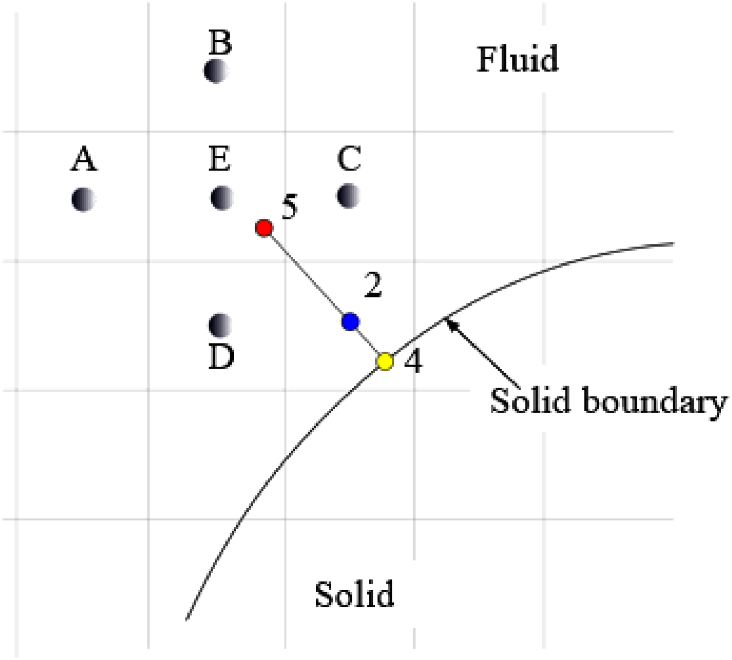
Sketch of the ghost-cell IBM.

The variables’ value at point 5 is calculated by the neighbored points in the fluid field, such as A, B, C, D, and E. (7 points for 3D calculation)

ϕ_{5} = ξ_{A} ϕ_{A} + ξ_{B} ϕ_{B} + ξ_{C} ϕ_{C} + ξ_{D} ϕ_{D} + ξ_{E} ϕ_{E}

(8)

where

ξ_{i}

is weight factor. The value at point 2 can be calculated based on the boundary conditions. For Dirichlet boundary condition,

ϕ_{2} = \frac{d_{g}}{d_{T} + d_{g}} ϕ_{4} + \frac{d_{T}}{d_{T} + d_{g}} ϕ_{5}

(9)

Where

d_{T}

is the distance between point 2 and point 4. For Neumann boundary condition,

ϕ_{2} = ϕ_{5} + {(\frac{δ ϕ}{δ n})}_{4} d_{g}

(10)

Then, the immersed boundary can be calculated.

Moving solid boundary

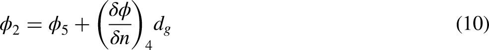
For the VAWT, the research on how to deal with the moving solid boundary is also necessary. It is due to the rotational blades that some mesh points are newly recognized as the fluid points or the near-wall fluid points while some are removed from the fluid field at every time step. It is shown in Figure 4 that the point n, which was in the solid at $T_{n}$ , is now identified to be included in fluid filed at $T_{n + 1}$ . Because the newly enrolled point n would join the immersed boundary calculation at $T_{n + 1}$ , it should value the point n at the first. As shown in Figure 4, the distance from point n to the solid surface can be re-calculated and point 4 can be marked on the solid surface based on the distance. Then, point n is taken as a mirror and the mirror point of point 4 can be found in the fluid field, marked by point 5. The variables’ value at point 5 is determined by the adjacent points and point 4. At last, point n is valued by point 5 and the boundary conditions.

Figure 4.

Fresh fluid nodes due to the moving solid boundary.

Validation of IBM

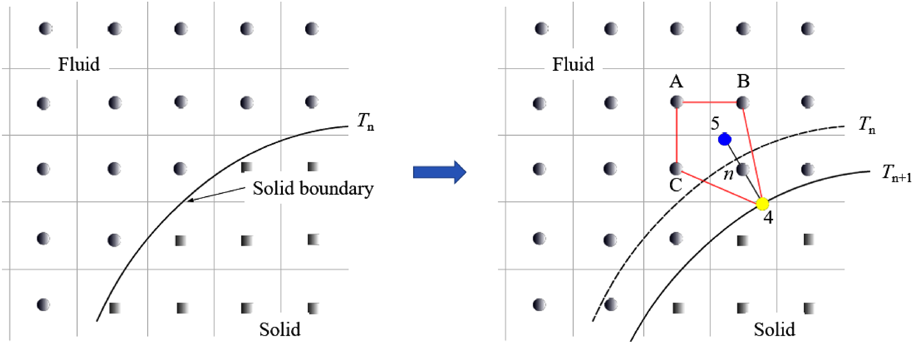
An in-house code, which had been applied to many research and industrial projects, has been modified according to the above-mentioned principles. In this paper, in order to evaluate the IBM, the flow filed around Eppler387 airfoil is studied. Eppler387 airfoil is one of the airfoils, which were usually applied to unmanned aerial vehicles. The profile of Eppler387 is shown in Figure 5. The computational zone of this case is 6C, 5C and 5C along stream-wise, broad-wise and span-wise correspondingly, where C is the chord length. The uniform orthogonal mesh is used. The total mesh is 99 million. The mesh structure and identified Eppler387 shape are shown in Figure 6. It is found that the impenetrable solid boundary can be well recognized by the IBM. As for the boundary conditions, incidence velocity and static pressure are applied to the inlet and the outlet boundary, respectively, other boundaries are set as solid wall. In this case, Reynolds number is about 1 × 10⁵ and attack angle is adopted as much as 4°.

Figure 5.

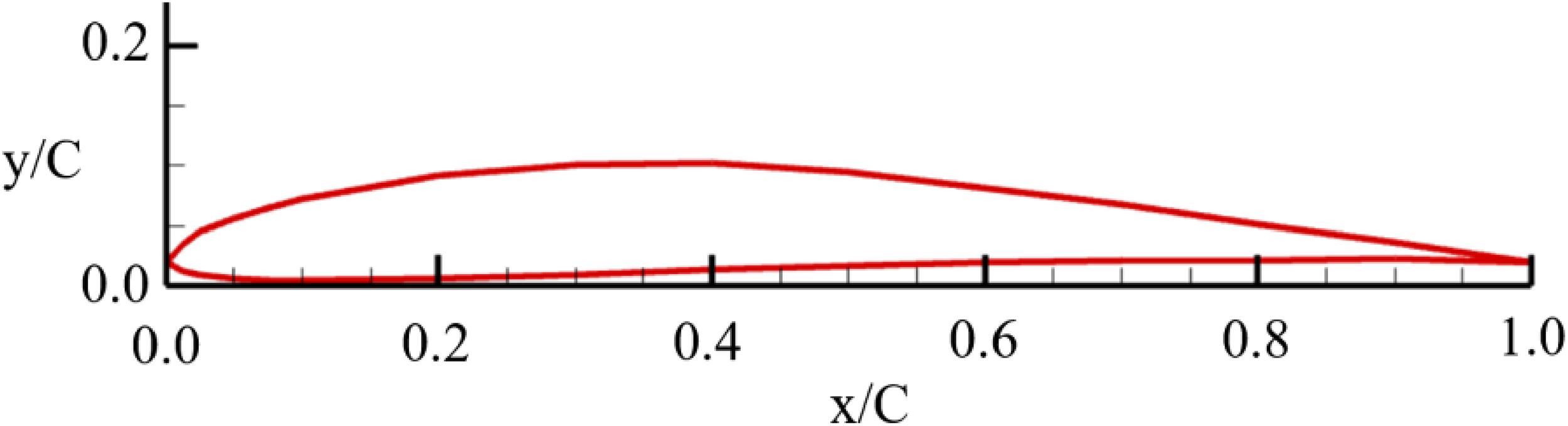
The profile of Eppler387.

Figure 6.

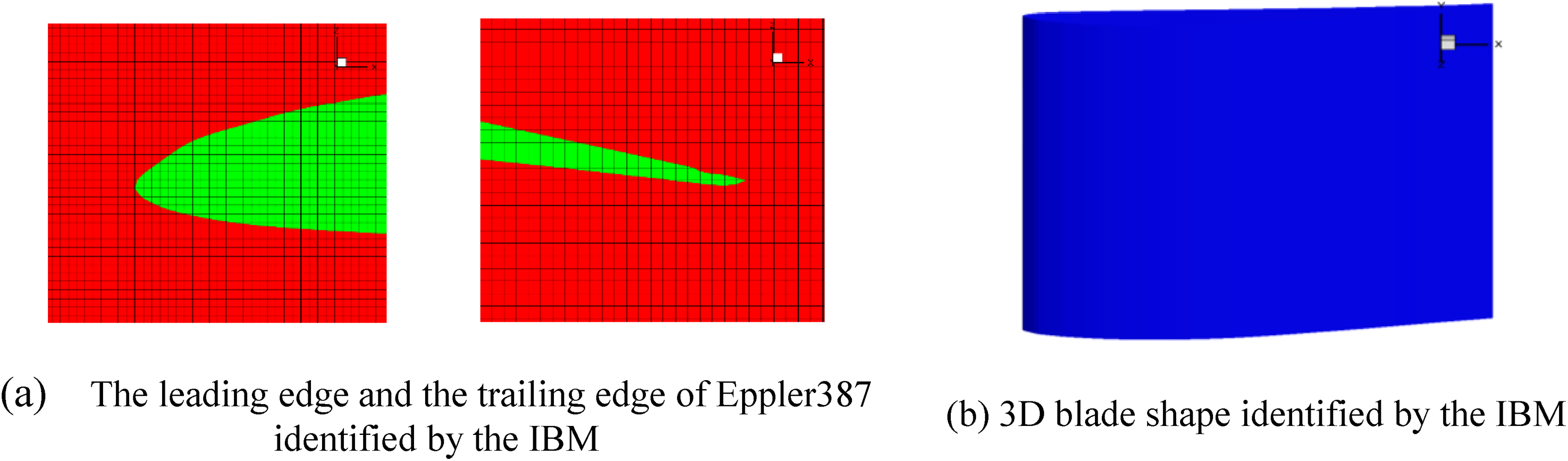
Solid boundary identified by the IBM.

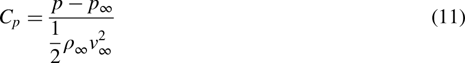
The comparison of pressure coefficient $C_{p}$ between experimental data (Mcghee et al., 1988) and results by the IBM is shown in Figure 7. $C_{p}$ is defined as the following.

C_{p} = \frac{p - p_{\infty}}{\frac{1}{2} ρ_{\infty} v_{\infty}^{2}}

(11)

Figure 7.

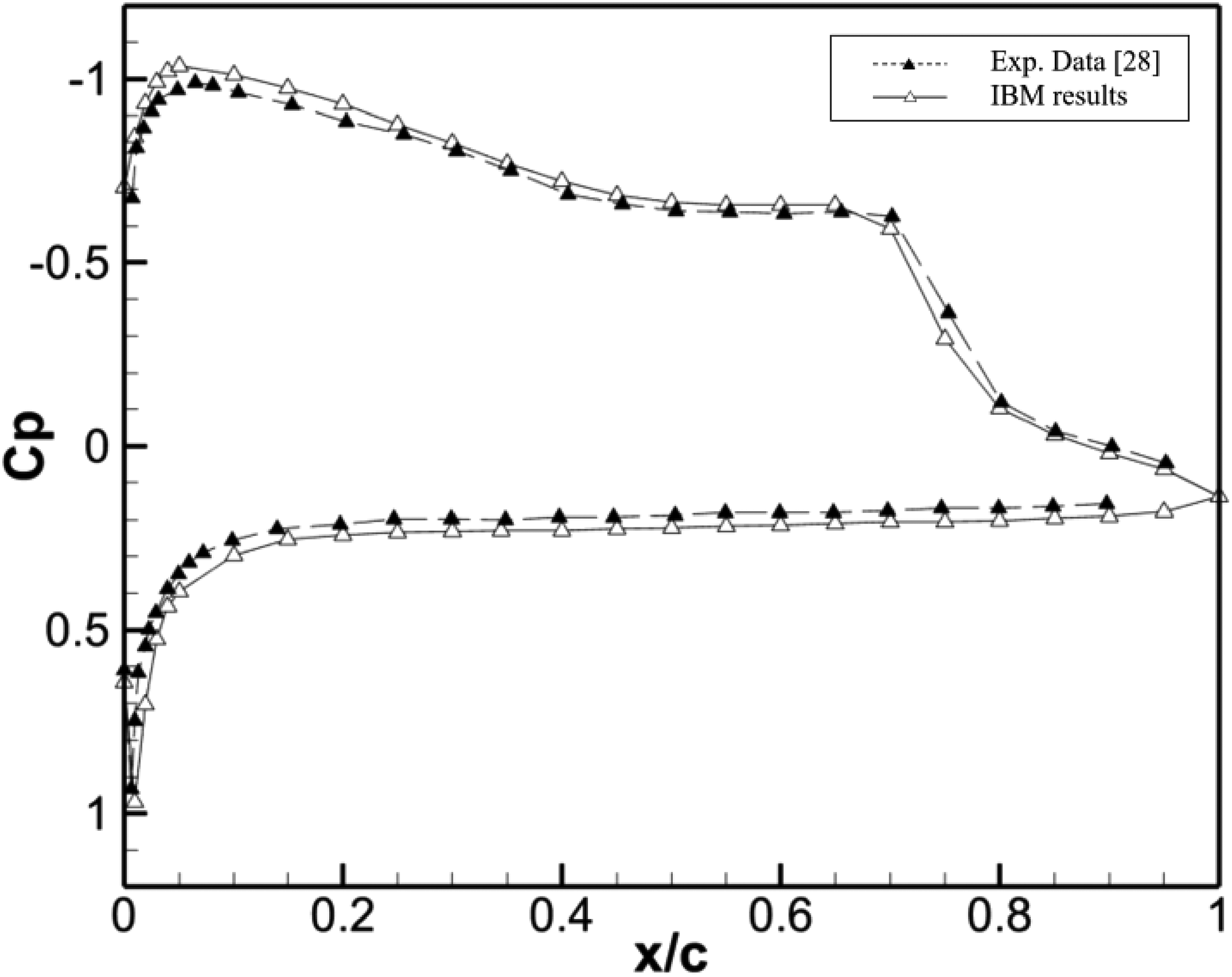
The comparison of C_p of Eppler387 between experimental data (Ghias et al., 2007) and IBM results.

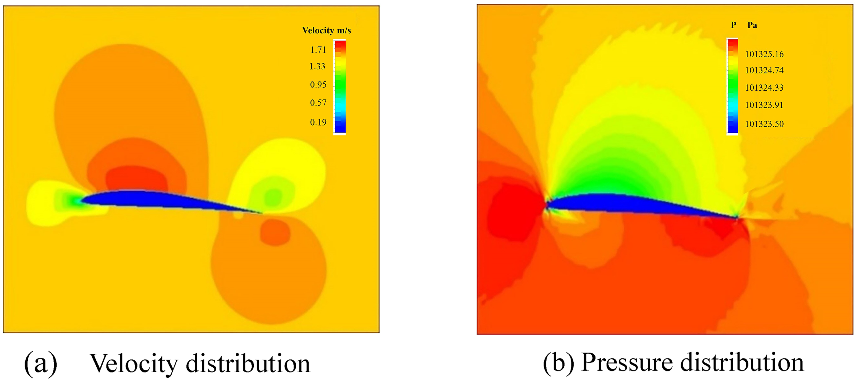
As shown in Figure 7, $C_{p}$ obtained from the IBM is agreed well with the experimental data. The maximum difference between two series of data is less than 3%, which can be reduced further when more fine mesh is adopted. The detail information of flow field is shown in Figure 8, in which the pressure and the velocity contours are presented. This flowing pattern shown in Figure 8 has been proved by many published works.

Figure 8.

Performance of Eppler387 from the IBM (Re: 1 × 10⁵, attack angle: 4°).

Numerical model

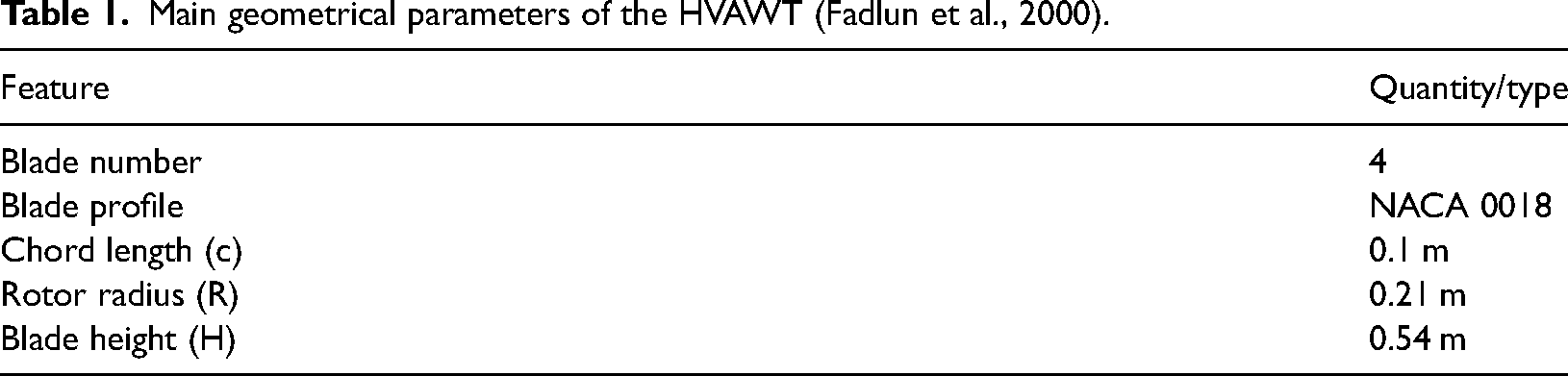
Referred to Cheng et al. (2017), the geometrical structure of a helical vertical axis wind turbine (HVAWT) studied in this paper is shown in Figure 9. It consists of four blades, which have a section of NACA0018 airfoil profile. The twisted angle of the wind turbine is 70°. The practical structure is shown in Figure 9(a). The simplified version without the struts is shown in Figure 9(b), which is taken as the model for the numerical simulation. The detailed geometrical parameters are shown in Table 1.

Figure 9.

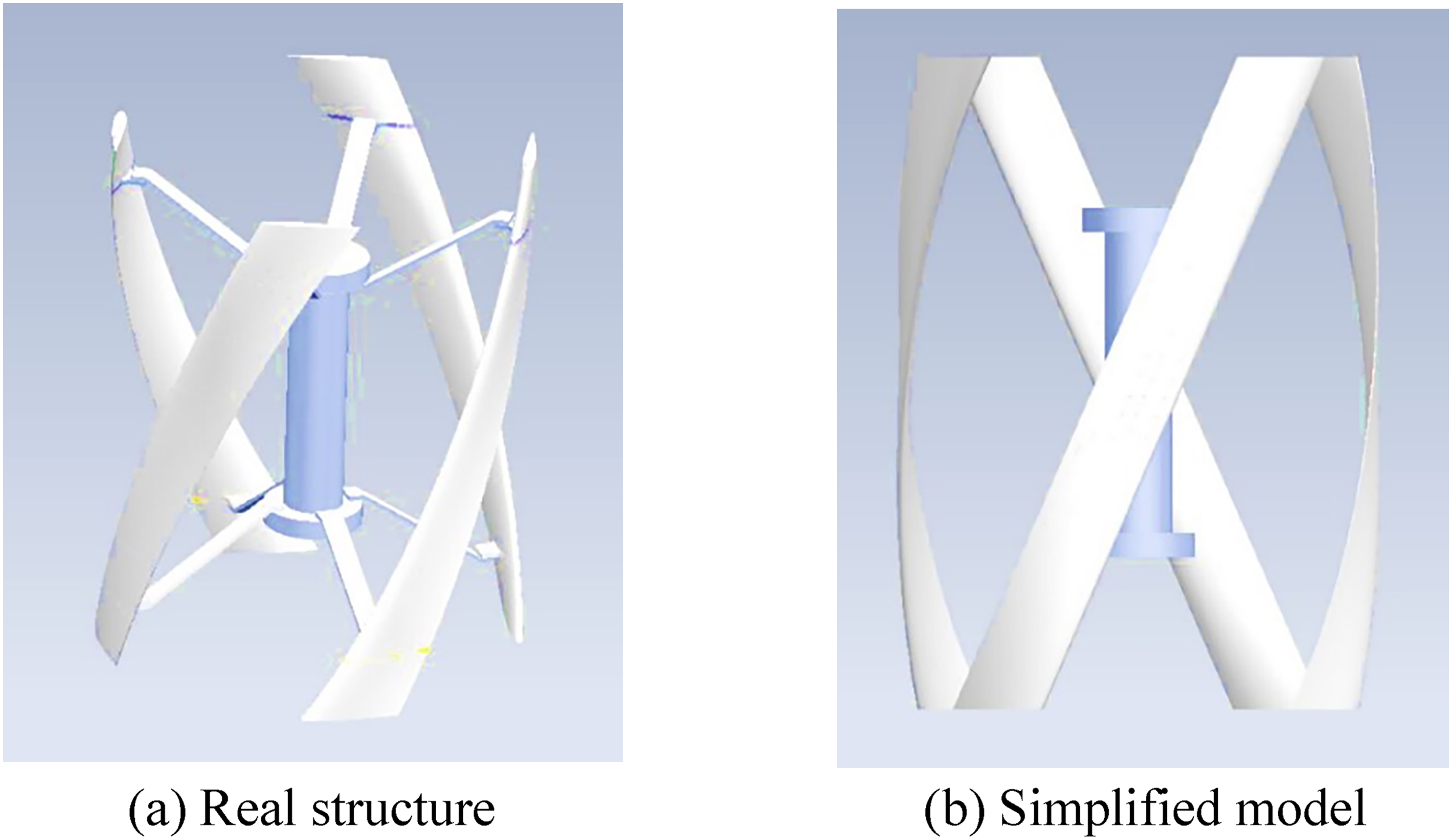
The geometrical structure of HVAWT.

Table 1.

Main geometrical parameters of the HVAWT (Fadlun et al., 2000).

Feature	Quantity/type
Blade number	4
Blade profile	NACA 0018
Chord length (c)	0.1 m
Rotor radius (R)	0.21 m
Blade height (H)	0.54 m

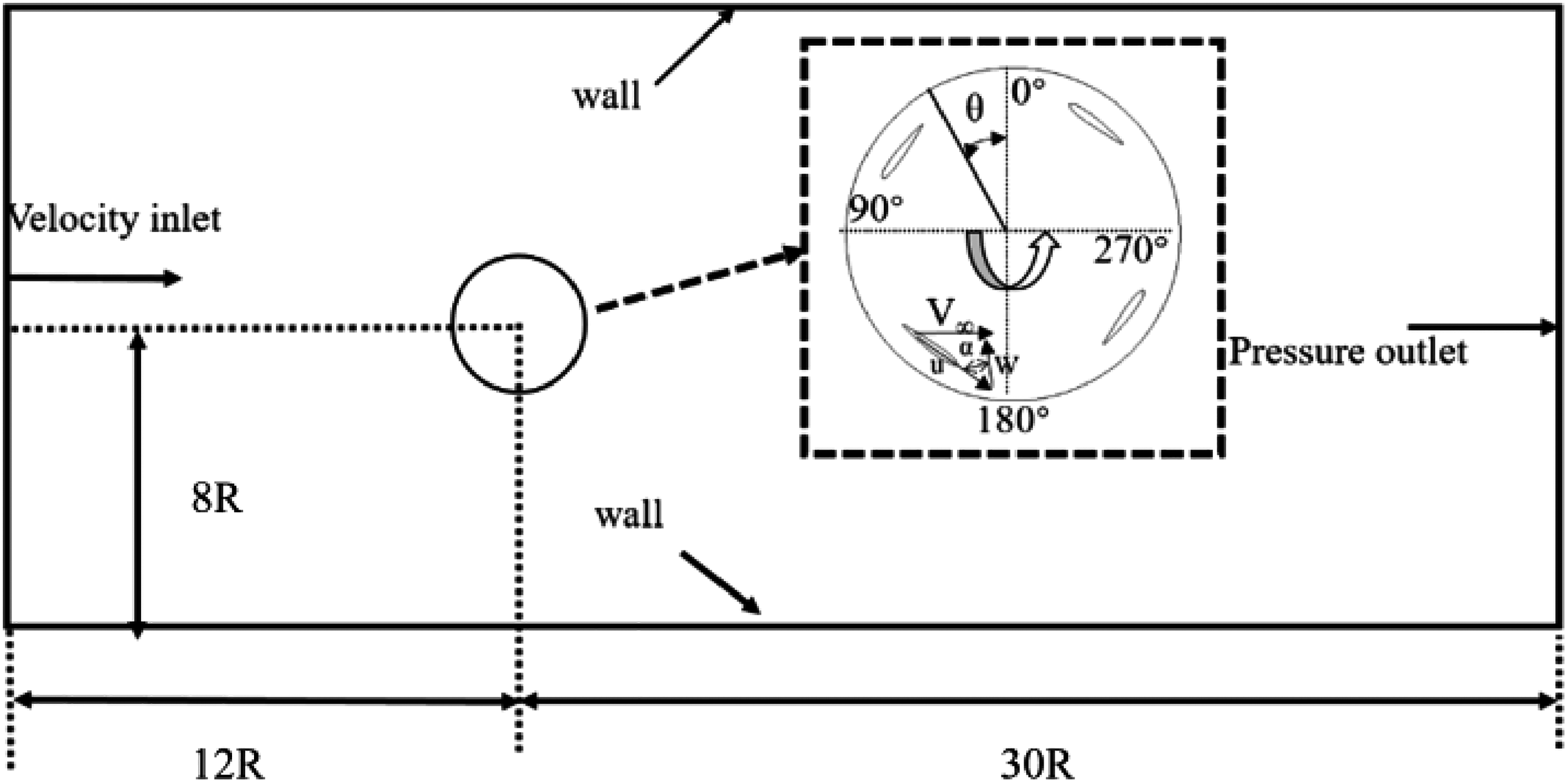
The computational zone is shown in Figure 10. In order to eliminate the effects of the inlet and the outlet boundary, the distance between two boundary and the center of HVAWT is extended to $12 R$ and $30 R$ respectively, where $R$ is the rotation radius of the wind turbine. Incidence velocity and static pressure are considered as inlet and outlet boundary conditions correspondingly. The incidence velocity adopted in this research is as much as $9.5 m \cdot s^{- 1}$ .

Figure 10.

The computational zone setup for HVAWT simulation.

In this case, a uniform mesh is applied to the spatial discretization and the total number of the mesh is about 550 million. The profile of HVAWT identified by the IBM is shown in Figure 11. It is shown that the 3D blade geometry has been accurately captured by the IBM with the adopted mesh density.

Figure 11.

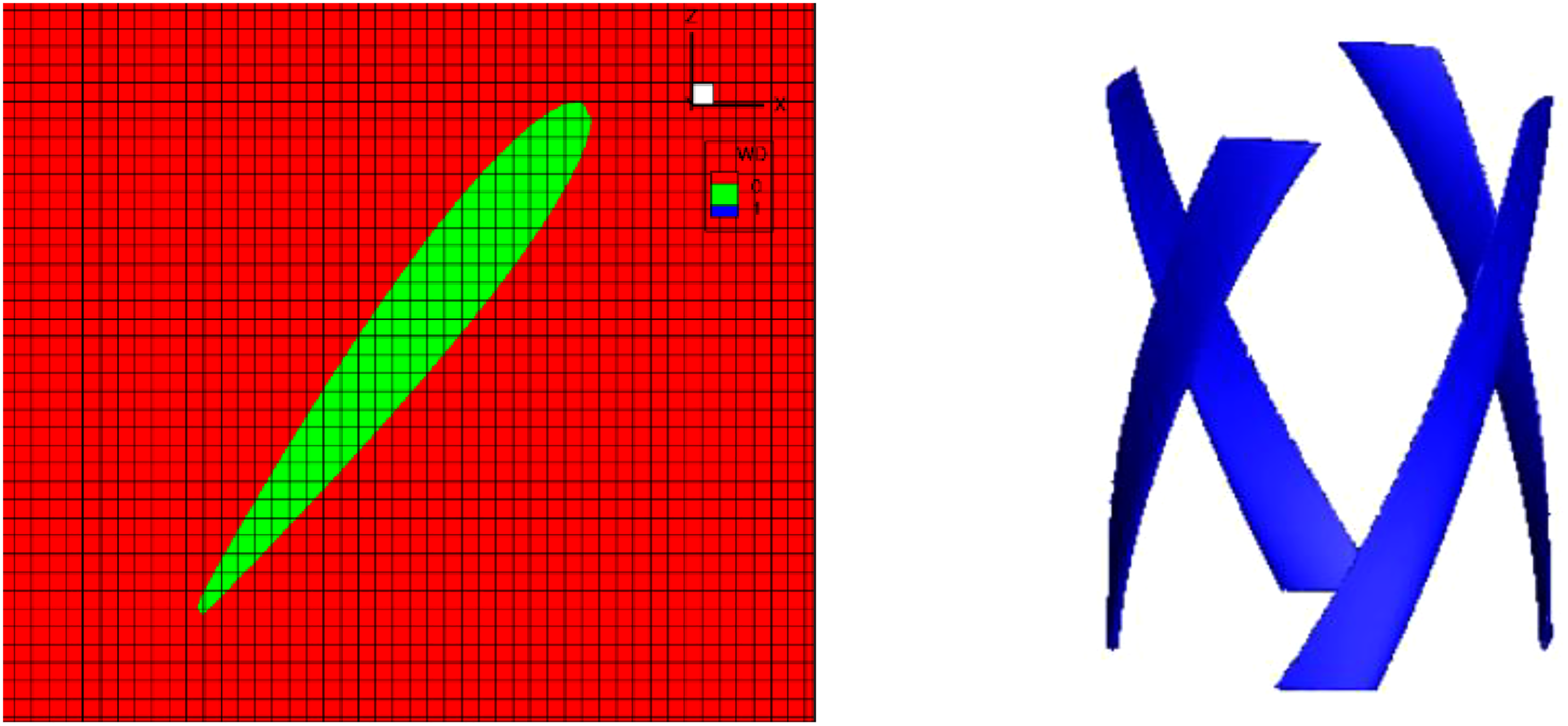
The uniform mesh structure and blade identification.

Result analysis

The comparison between the IBM and the body-fitted mesh method

Power coefficient

Power coefficient, $C_{P t}$ , is always considered as a critical parameter to evaluate the aerodynamic performance of a wind turbine. It can be defined as the following.

C_{P t} = \frac{P}{W} = \frac{Γ ω}{1 / 2 ρ D H V_{\infty}^{3}}

(12)

where

Γ

is the torque output of a wind turbine,

ω

the rotational speed,

V_{\infty}

the incidence velocity, H the height of the turbine and D the rotor diameter. For the IBM, the total torque is calculated based on the pressure of the MPs distributed on the entire blade surface.

In order to check the accuracy of the IBM and evaluate whether it is suitable to the flowing simulations of HVAWT or not, the numerical calculation is also carried out based on 3D unsteady DES with a body-fitted mesh (BFM). The computational domain is the same as that adopted in the calculation of the IBM. But, the whole domain is divided into several blocks and all blocks are connected by non-conformal interfaces. And the sliding mesh technology is applied to these interfaces to finish the data transferring among the blocks. Based on the research of the grid dependence on the mesh scale and the time step, the total grid point for the 3D unsteady DES is about 70 million. The time step is as much as $Δ t = T / 200$ . And the turbulence model of k-ω SST is adopted to close the governing equations.

Both power coefficient from the BFM and the IBM are shown in Figure 12. According to the figure, the average power coefficient obtained from the BFM is about 0.159 while the average coefficient by the IBM is 0.148. Compared with the experimental data (Heo et al., 2016), the error of the BFM is about 5.3% and is only 1.3% for the IBM. It demonstrates that the IBM is more beneficial to the unsteady numerical simulation with the moving solid boundary. Meanwhile, it is noted that there is phase difference between the IBM and the BFM with the same boundary conditions. The detailed information on the flowing field will be discussed in the next section.

Figure 12.

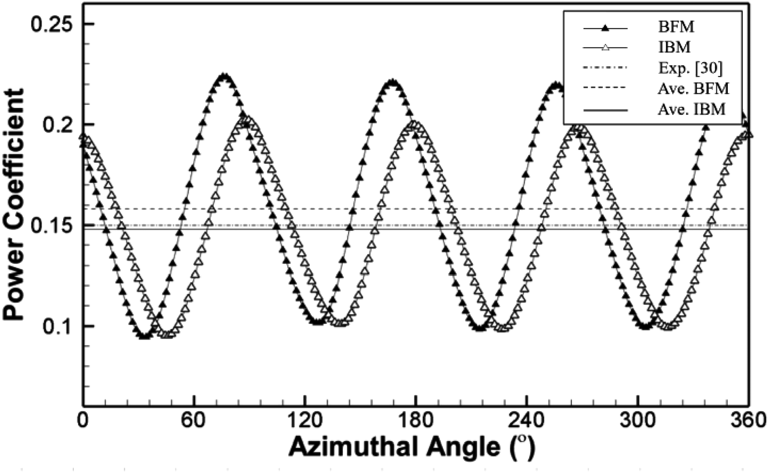
Power coefficient comparison.

Flow detail comparison

In order to explain the power difference predicted between the BFM and the IBM, 3D vortex core regions from two methods based on the Q-Criterion are shown in Figure 13. According to the figure, the vorticity strength from the IBM is obviously stronger than that from the BFM. It is due to the stronger vortex found in Figure 13(b) that the viscous loss is increased and hereupon the power coefficient is affected negatively. Furthermore, at two ends of the blade, the downwash vortex can be observed easily, as shown in Figure 14. The vortex is formed due to the pressure difference between suction surface and pressure surface and can reduce the power output substantially. But this phenomenon is not obvious in the results from the BFM.

Figure 13.

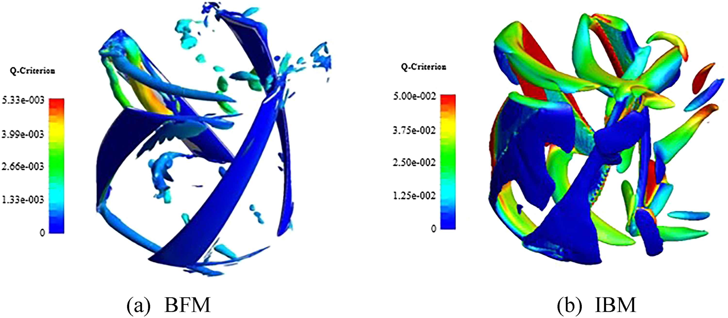
Vorticity contours based on the Q-Criterion.

Figure 14.

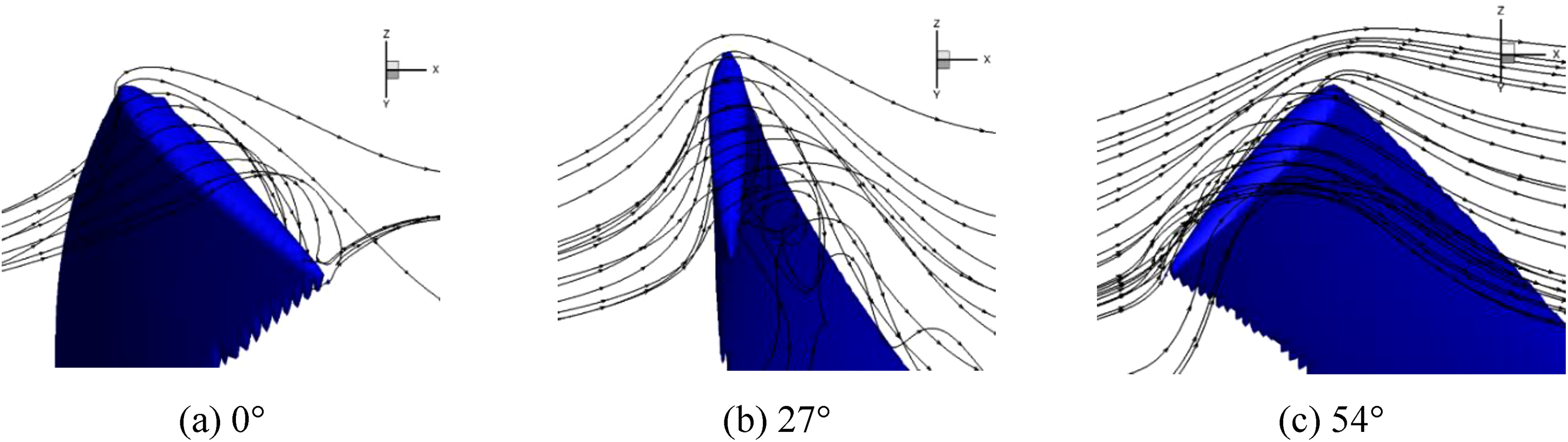
Streams at the top of the blade from the IBM.

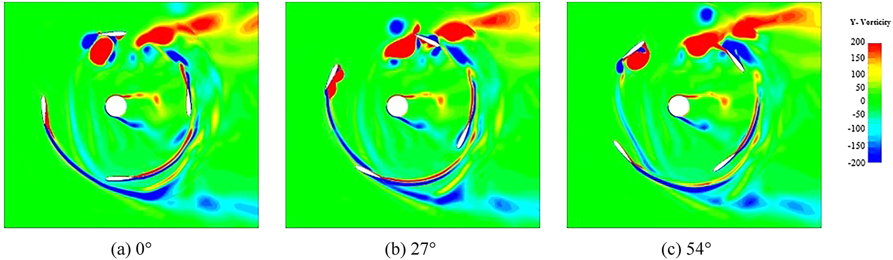
The vorticity contours at the mid-span are shown in Figures 15 and 16, respectively. As shown in Figure 15, the strength of the detached eddies is so small that region affected by these eddies is very limited. However, the situation for the IBM is totally different and the affected region is enlarged from upstream to downstream shown in Figure 16.

Figure 15.

Vorticity contours at the mid-span from the BFM.

Figure 16.

Vorticity contours at the mid-span from the IBM.

It is believed that the results difference is attributed to the mesh strategy. In the BFM, the computational domain is divided into two different zones and the data exchanging on the interface between two zone depends on the sliding mesh technology. Unfortunately, two blade ends and the wake of the blades are very close to the interface. In these regions, the gradient of physical parameters is not small and unsteady characteristics is dominant. So, some valuable unsteady information might be omitted or averaged during the process of the data exchanging. Compared with the BFM, the solid boundary is replaced by the immersed boundary so that the data is exchanged among the nodes without any interfaces. Thus, some important information on the flow field has been preserved completely, especially for the unsteady flow field.

Influence of blade shape on the VAWT performance

The other kind of VAWT, called straight blade vertical axis wind turbine (SVAWT), also attracts more and more interests due to its simpler structure. In order to evaluate the effect of blade shape on the power output of a VAWT, the numerical simulations of the SVAWT based on the IBM are also carried out in this paper. The geometrical structures of the SVAWT identified by the IBM is shown in Figure 17. All boundary conditions and the meshing remain the same as those used in the case of the HVAWT, but the MPs are re-allocated according to the shape of the blade.

Figure 17.

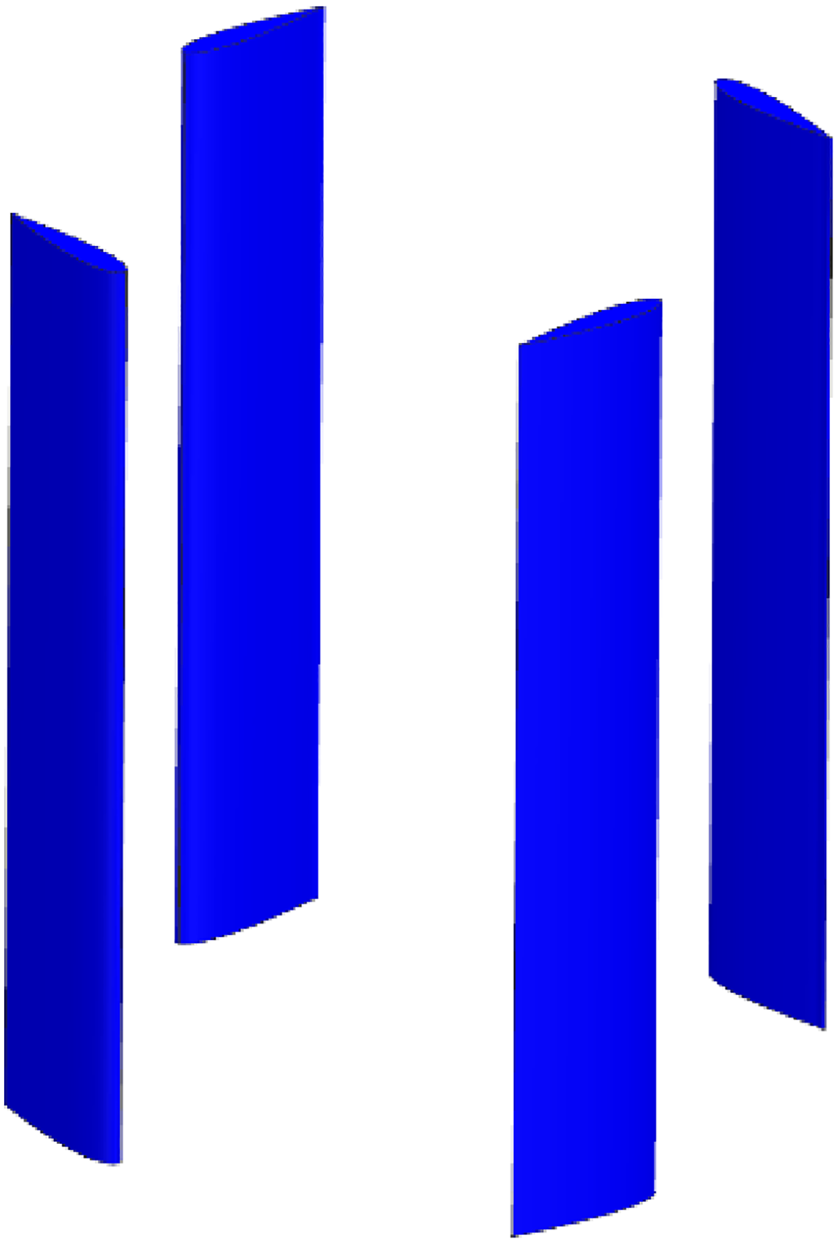
SVAWT identified by the IBM.

Power coefficient

The power coefficient of the HVAWT and the SVAWT are shown in Figure 18. The averaged power coefficient of the SVAWT has 2% higher than that of the HVAWT. Meanwhile, there is a little phase difference between two turbines. It demonstrates that the straight blade can extract more power from incidence flow than that from the helical blade.

Figure 18.

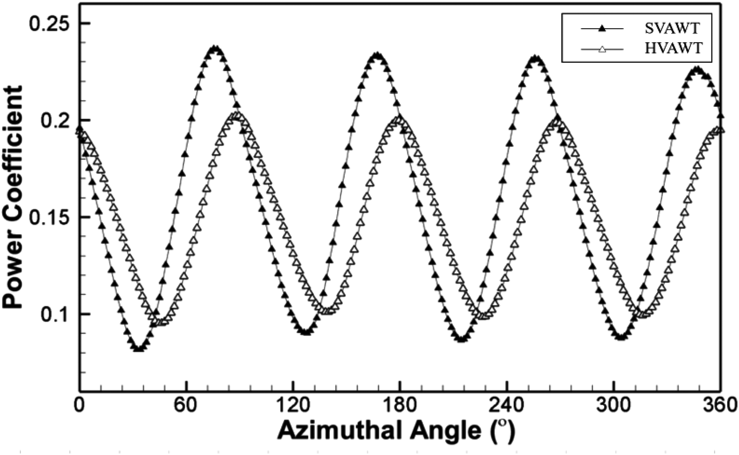
Power coefficient of HVAWT and SVAWT based on the IBM.

The fluctuation factor is very important to the power generation. The factor 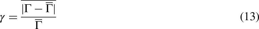$γ$ is defined as

γ = \bar{\frac{| Γ - \bar{Γ} |}{\bar{Γ}}}

(13)

where

Γ

is the instant torque and

\bar{Γ}

is the average torque in a revolution. If it was too large, there would be a big problem to the mechanical wear of a wind turbine and the service life of energy converting systems would be affected negatively. The factor of the HVAWT is about 20.9% while 28.5% for the SVAWT. It means that the SVAWT would have to face more serious stability challenge and to tolerate more aerodynamic instability than those for the HVAWT. Furthermore, this situation would be deteriorated with the increasing of the velocity of the incidence flow.

By the way, for the HVAWT, one of its advantages is insensitive to the direction of the incidence flow. In other words, when the direction of the incidence flow is changed, its rotation direction remains the same. It is beneficial to the installing and the routine maintenance of a wind turbine.

Detail flowing comparison

The velocity contours on the sections of the blade height 80% are shown in Figures 19 and 20. It indicates that compared with the HVAWT, the interaction between the fluid and the blades of the SVAWT is stronger and the power output is more obtained. But, the corresponding negative results is more complex fluid field and thereby more fluctuated output, which is agreed with the above presented data and analysis.

Figure 19.

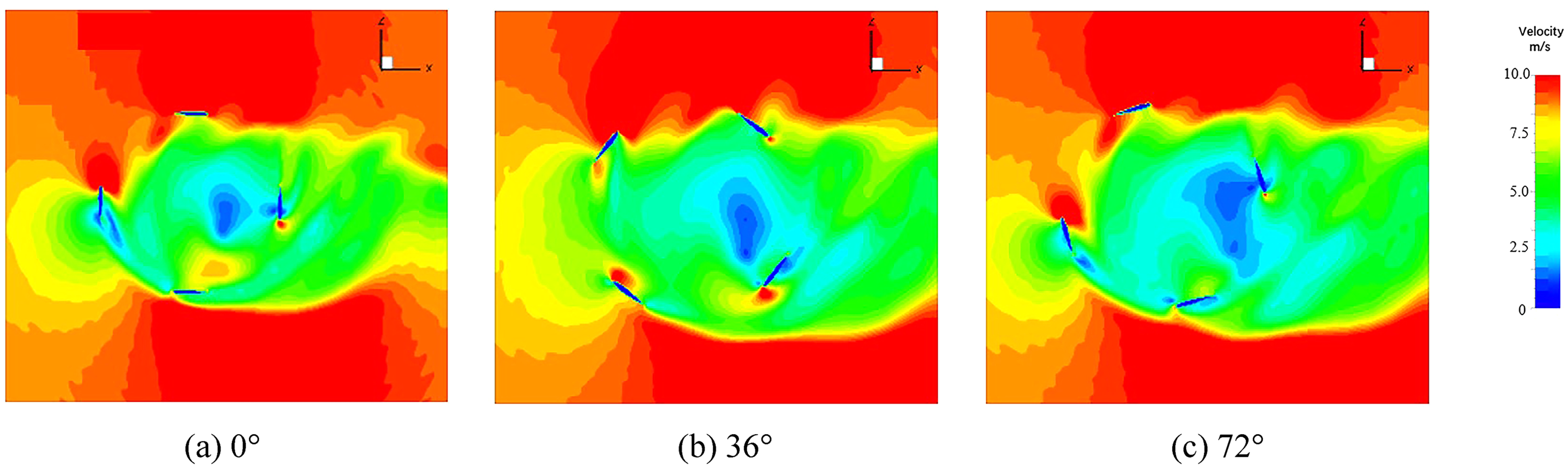
Velocity contours of the HVAWT.

Figure 20.

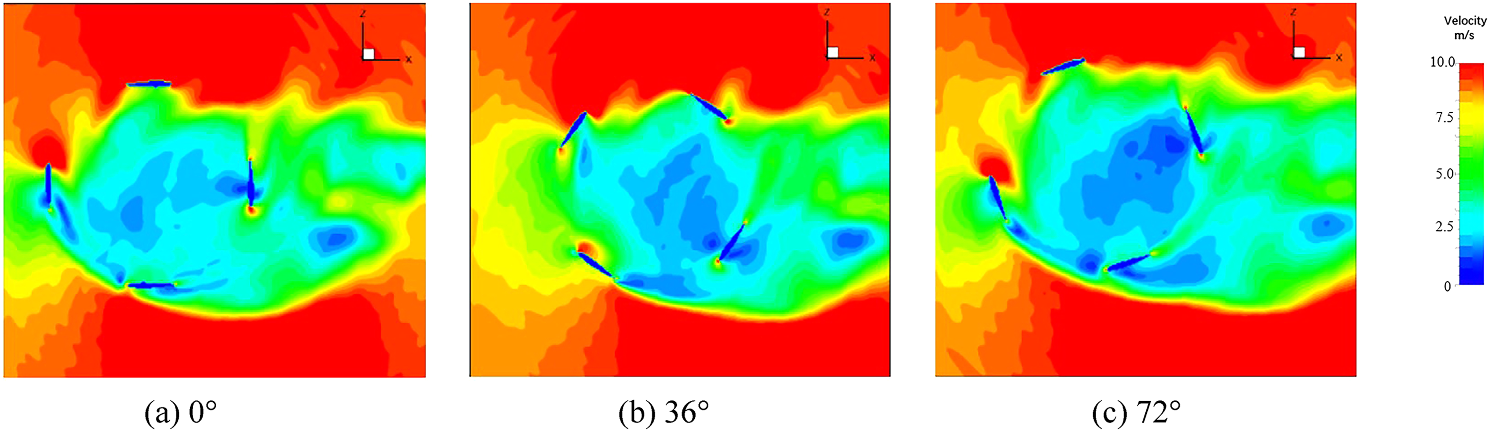
Velocity contours of the SVAWT.

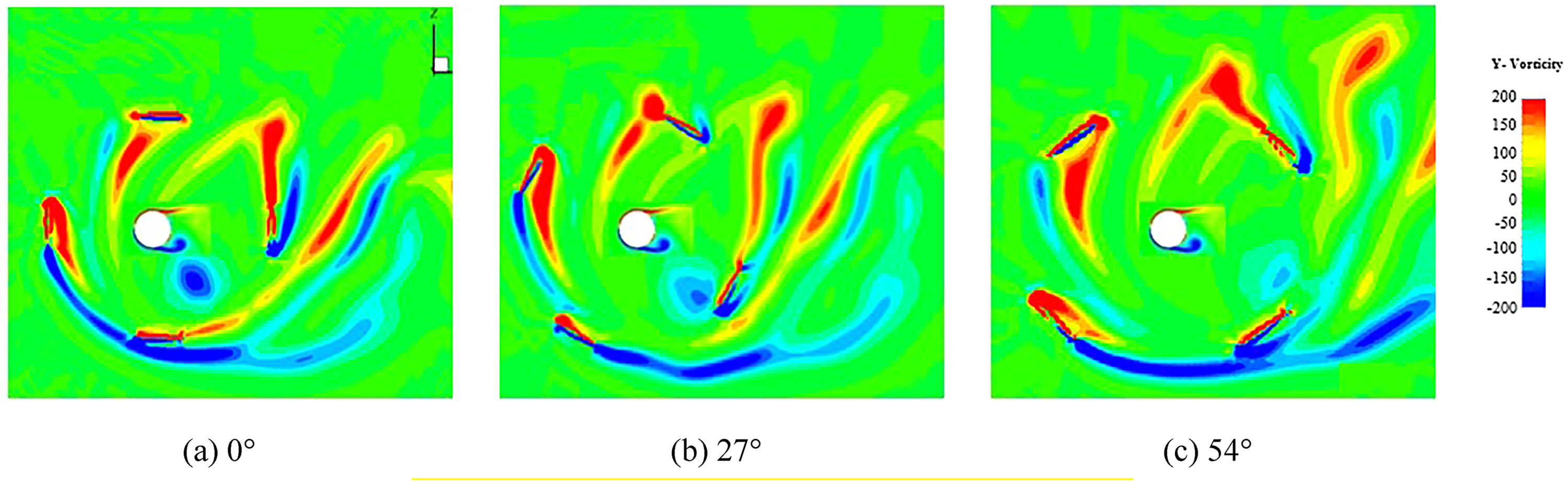
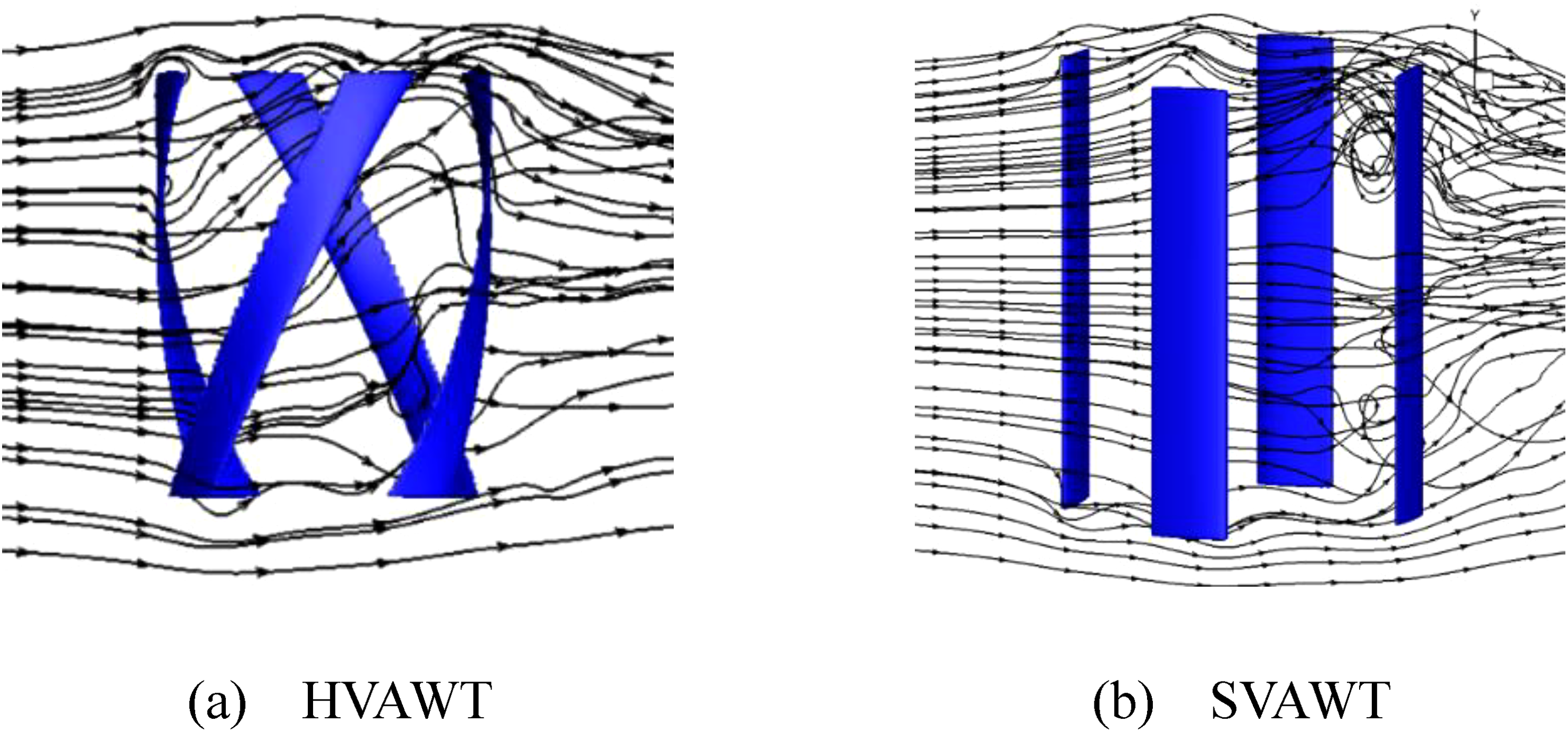
The vorticity contours along the blade height direction are shown in Figures 21 and 22. At two blade ends of both turbines, tip vortices can be identified. These vortices are regularly shed from the blades into the wake region. Furthermore, it is due to the straight blade of the SVAWT that the tip vortices as well as the shed vortices present perfect symmetry at two ends of the blades. When a turbine is rotated, there is pressure difference between inner domain (surrounded by the blades) and outer domain. On the plane of revolution, the pressure difference is balanced by the centrifugal force. But in the blade height direction, the pressure difference is considered as the main force to push the secondary flowing. For the HVAWT, its helical blade can guide and promote this kind of flowing. But the straight blades are barriers to the flowing. The same phenomena can be also observed in the Figure 23, in which 3D streamlines are shown. It is found that there is the secondary flowing around the helical blades while for the straight blades this kind of flowing is not obvious. Meanwhile, it is due to the secondary flowing that the flow field of the HVAWT downstream becomes more uniform in the blade height direction and the fluctuation of the aerodynamic parameters is mitigated to some degree.

Figure 21.

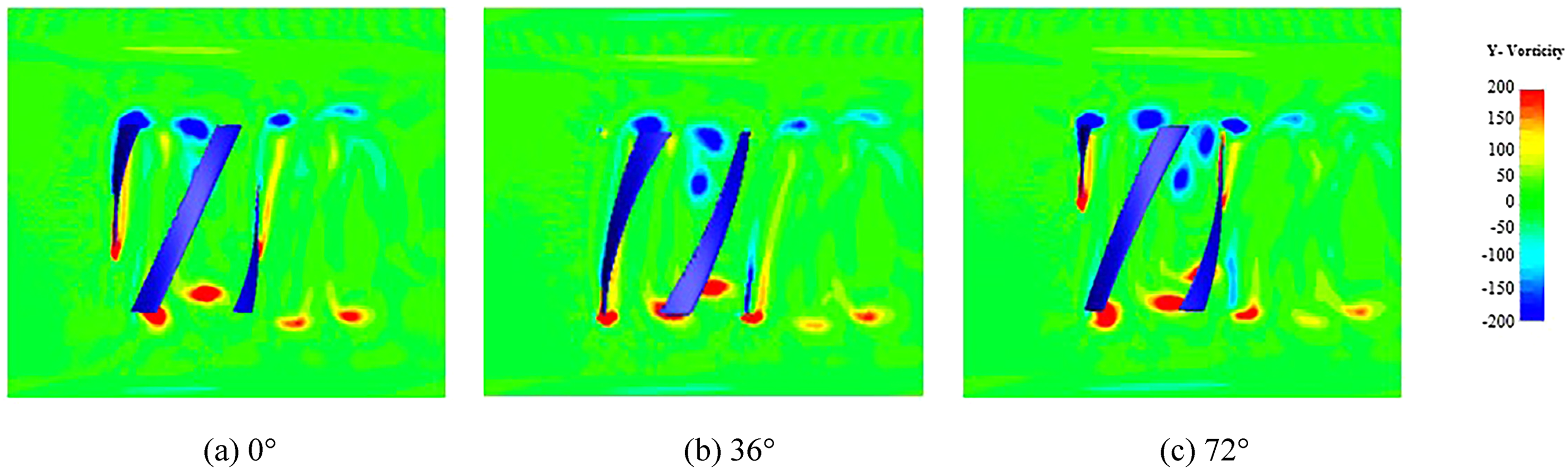
Vorticity contours of the HVAWT.

Figure 22.

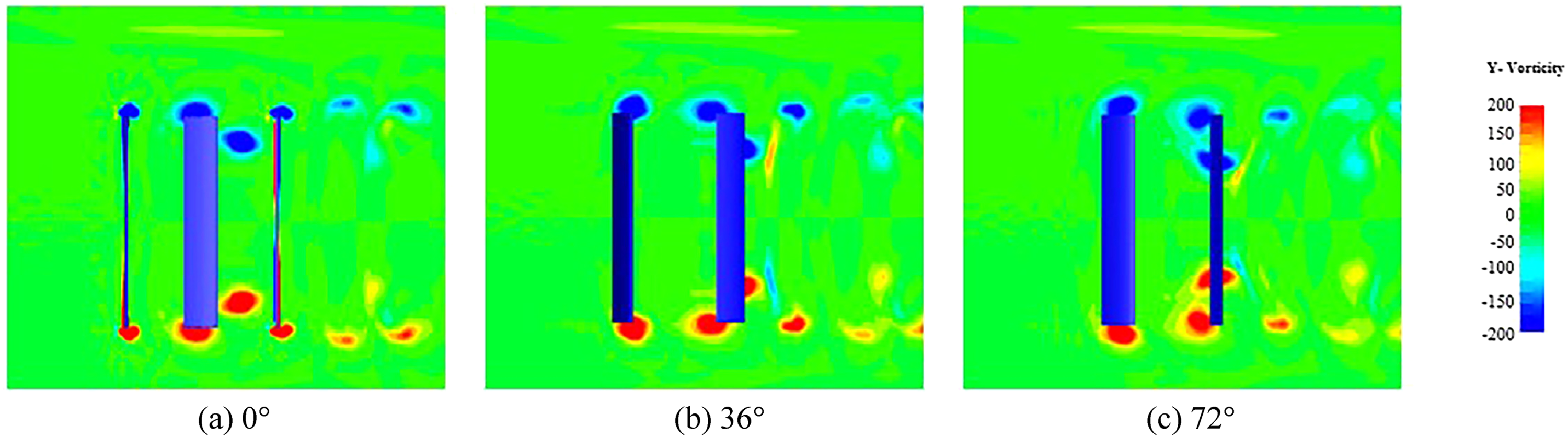
Vorticity contours of the SVAWT.

Figure 23.

3D streamlines of HVAWT and SVAWT (72°).

Discussion

Unlike the body-fitted mesh, in the IBM much more time spends on the identifying of the solid boundary. In addition, in order to improve the calculation accuracy, the mesh refinement in the regions neighbored the blades needs to be carried out and then brings about the sharply increasing of the grid number. By the way, in the calculation strategy of the moving boundary, the accuracy of the IBM suffers from too much new collected fluid points at a time step. Thus, the time step is smaller than that adopted in the traditional numerical simulation. So, the calculation consumption of the IBM is so high that no practical design or application can stand such high consumption. The problem of the calculation resource is not avoidable for the IBM research though the method can bring more detailed results and make researchers get more understanding on the characteristics of the turbines. All the same, we believe that when the computer technology is developed to a stage that calculation source is no longer to be considered as a barrier in the recent future, the IBM will be widely applied to the aerodynamic numerical simulation of the wind turbine indeed.

Conclusion

The basic aim of this research is to find a method, by which the performance of a kind of VAWT can be evaluated more accurately and efficiently. To this end, a discrete cell method, or ghost-cell IBM, has been introduced into an in-house flow solver, which is believed to be suitable to the numerical simulation of the VAWT. Moreover, particular efforts have been focused on the mesh scheme for the moving solid boundary. The following items are summarized on the current state of the art of methodology of the performance estimating of the wind turbine, and demonstrate the perception of researchers in the field of numerical simulation:

It has been validated that the ghost-cell discrete forcing IBM is suitable to the performance estimation of the VAWT.

The sliding mesh technology is substituted by the mesh scheme for the moving solid boundary in the IBM so that the unsteady flow information is not disturbed by the mesh problem and is reserved completely.

Unlike the body-fitted mesh, in the IBM much more time spends on the identifying of the solid boundary and the refining of the mesh. So, the calculation consumption of the IBM is high a little bit.

By the using of IBM, the solid boundary is replaced by the immersed boundary so that the data is exchanged among the nodes without any interfaces. Thus, some important information on the flow field has been preserved completely, especially for the unsteady flow field.

Furthermore, the effect of the blade shape on the power output is studied based on the comparison of the HVAWT and SVAWT. Though the averaged power coefficient of the SVAWT has 2% higher than that of the HVAWT, the HVAWT has a fair advantage on the operating stability.

Highlights

A discretized forcing type IBM is introduced to study VAWT.

The ghost-cell discrete forcing IBM is suitable to the performance estimation of the VAWT.

The HVAWT has an advantage on the operating stability.

Footnotes

Declaration of conflicting interests

The author(s) declared no potential conflicts of interest with respect to the research, authorship, and/or publication of this article.

Funding

The author(s) disclosed receipt of the following financial support for the research, authorship, and/or publication of this article: This research is funded by the National Key R&D Program of China (No. 2019YFB1503700).

ORCID iD

Bo Yang

Appendix

References

Barba

Stoesser

(2017) An immersed boundary-based large-eddy simulation approach to predict the performance of vertical axis tidal turbines. Computers & Fluids 152: 74–87.

Cameron

Sheikh

Sean

, et al. (2023) 3D CFD modelling of performance of a vertical axis turbine. Energies 16(3): 1144.

Castiglioni

Domaradzki

Pasquariello

, et al. (2014) Numerical simulations of separated flows at moderate reynolds numbers appropriate for turbine blades and unmanned aero vehicles. International Journal of Heat & Fluid Flow 49: 91–99.

Chen

Lian

(2015) Numerical investigation of vortex dynamics in an H-rotor vertical axis wind turbine. Engineering Applications of Computational Fluid Mechanics 9(1): 21–32.

Cheng

Liu

, et al. (2017) Aerodynamic analysis of a helical vertical axis wind turbine. Energies 10(4): 575.

Das

Banerjee

Mondal

(2021) A comparative CFD study to analyze the performance of NACA 0018 and S1210 darrieus wind turbine blade. Fluid Mechanics and Fluid Power (Vol. 2). FMFP 2021. Lecture Notes in Mechanical Engineering. Singapore: Springer, pp. 279–284.

Fadlun

Verzicco

Orlandi

, et al. (2000) Combined immersed-boundary finite-difference methods for three-dimensional complex flow simulations. Journal of Computational Physics 161(1): 35–60.

Ferreira

Kuik

Bussel

(2006) Wind tunnel hotwire measurements, flow visualization and thrust measurement of a VAWT in skew. Journal of Solar Energy Engineering 128(4): 487–497.

Gaikwad

Maity

Ghaisas

(2021) Implementation of a ghost-point immersed boundary method in a high-order finite-difference large-eddy simulation code. Fluid Mechanics and Fluid Power (Vol. 3). FMFP 2021. Lecture Notes in Mechanical Engineering. Singapore: Springer, pp. 97–102.

10.

Ghias

Mittal

Dong

(2007) A sharp interface immersed boundary method for compressible viscous flows. Journal of Computational Physics 225(1): 528–553.

11.

Giahi

Bergstrom

(2023) A critical assessment of the immersed boundary method for modeling flow around fixed and moving bodies. Computers & Fluids 256(4): 105841.

12.

Heo

Choi

Kim

(2016) CFD And experiment validation on aerodynamic power output of small VAWT with low tip speed ratio. Journal of the Korean Society of Marine Engineering 40(4): 330–335.

13.

Howell

Qin

Edwards

, et al. (2010) Wind tunnel and numerical study of a small vertical axis wind turbine. Renewable Energy 35(2): 412–422.

14.

Huang

Carlos

(2022) An immersed boundary method with implicit body force for compressible viscous flow. Journal of Computational Physics 459(6): 111125.

15.

Indhumathy

Mahalakshmi

(2022) 3D-CFD Flow driven performance analysis of new non-cylindrical helical vertical axis wind turbine for fluctuating urban wind conditions. Energy Sources, Part A: Recovery, Utilization, and Environmental Effects 44(1): 2186–2207.

16.

Lida

Kato

Mizuno

(2007) Numerical simulation of unsteady flow and aerodynamic performance of vertical axis wind turbines with LES. Proceedings of the 16th Australasian Fluid Mechanics Conference (AFMC), The University of Queensland.

17.

Liu

Yang

, et al. (2018) Research on the turbine blade vibration base on the immersed boundary method. ASME Journal of Fluids Engineering 140(6): 061402.

18.

Mcghee

Walker

Millard

(1988) Experimental results for the Eppler 387 airfoil at low Reynolds numbers in the Langley Low-Turbulence Pressure Tunnel. NASA Report, TM-4062.

19.

Mohd

Syed

Naik

(2023) Comparative analysis of low velocity vertical axis wind turbine NACA blades at different attacking angles in CFD. Materials Today: Proceedings 8: 2091–2100.

20.

Nguyen

(1979) A Vortex model of the Darrieus turbine. USA: Master's Thesis, Texas Tech University.

21.

Pedram

Gholamhassan

Barat

, et al. (2023) CFD-study of the H-rotor darrius wind turbine performance in drag-lift and lift regime: Impact of type, thickness and chord length of blades. Alexandria Engineering Journal 67(3): 51–64.

22.

Peskin

(1977) Numerical analysis of blood flow in the heart. Journal of Computational Physics 25(3): 220–252.

23.

Strickland

(1975) The Darrieus turbine: a performance prediction model using multiple streamtubes. Sandia Laboratory Rept. SAND 75-0431. Sandia National Laboratories, Albuquerque, New Mexico.

24.

Tay

Deng

Oudheusden

BWV

, et al. (2015) Validation of immersed boundary method for the numerical simulation of flapping wing flight. Computers & Fluids 115: 226–242.

25.

Templin

(1974) Aerodynamic performance theory for the NRC vertical-axis wind turbine. NASA Sti/recon Technical Report N, 76.

26.

Wang

Zhou

(2022) A hybrid immersed-boundary/body-fitted-grid methodand its application to simulating heart valve flows. International Journal for Numerical Methods in Fluids 94(12): 1996–2019.

27.

Wang

Cao

(2022) Numerical study of aerodynamic roles of bridge railings by immersed boundary method. Journal of Wind Engineering and Industrial Aerodynamics 228(9): 105111.

28.

Wolfe

Ochs

(1997) Predicting aerodynamic characteristic of typical wind turbine airfoils using CFD. Sandia Laboratory Rept. SAND 96-2345. Sandia National Laboratories, Albuquerque, New Mexico.

29.

Huang

(2023) Kinetic modeling of immersed boundary layer for accurate evaluation of local surface stresses and hydrodynamic forces with diffuse interface immersed boundary method. Physics of Fluids 35: 043609.

30.

Chen

H-C

Koop

(2023) High-fidelity CFD simulations for the wake characteristics of the NTNU BT1 wind turbine. Energy 266, No. 126285.

The study of vertical-axis wind turbine based on immersed boundary method

Abstract

Keywords

Introduction

Numerical method

Governing equations

Immersed boundary method

Points identification

Immersed boundary conditions

Moving solid boundary

Validation of IBM

Numerical model

Result analysis

The comparison between the IBM and the body-fitted mesh method

Power coefficient

Flow detail comparison

Influence of blade shape on the VAWT performance

Power coefficient

Detail flowing comparison

Discussion

Conclusion

Highlights

Footnotes

Declaration of conflicting interests

Funding

ORCID iD

Appendix

References