
Abstract
A commingled production scheme, where wells are simultaneously completed in multiple reservoir units, offers a cost-effective alternative worldwide. However, their behavior can be more complex than single-unit wells in sequential production. Limited completion studies exist for the unique Paleogene Gulf of Mexico fields. To aid decision-making, we conducted a numerical study using geological and reservoir models of Lower and Upper Wilcox units, based on publicly available data. Results show that commingled production maximizes per-well oil production compared to sequential schemes. Over 30 years, it provides 61% more oil recovery, and over 50 years, it yields 21% more. One-factor-at-a-time design of experiments sensitivity analysis identifies that key reservoir properties influencing oil recovery in both schemes are upper and lower unit thicknesses, facies proportion of the upper unit. Additionally, average permeability of the lower unit plays a significant role in sequential production schemes.
Keywords
Introduction
Due to the high cost of offshore drilling, economically feasible petroleum resource development requires the reuse of wells for production over multiple stacked reservoir intervals. Two alternatives are sequential production schemes, the recompletion and production over a series of reservoir intervals one-at-a-time, or commingled production schemes, the completion and simultaneous depletion over multiple reservoir intervals. Because of its benefits like simplicity, reliability, lower cost, and ease of well intervention, commingled production schemes are a practical approach to developing offshore reservoirs (Al-Shehri et al., 2005). Commingled production schemes accelerate well and field production over time, extend the economic life of wells and, as a result, often increase the net present value of a petroleum resource project (Hoy et al., 2016). Although there are many advantages of a commingled production scheme, it may result in reservoir management challenges. Production performance is not the same between single-reservoir and multi-reservoir interval wells; therefore, the evaluation of commingled well performance is more challenging (Vo and Madden, 1995). Depending on the specific properties of each reservoir interval and the entire reservoir along with operational parameters, depletion occurs at different rates (Eskandari et al., 2012). Higher productivity and higher quality reservoir intervals may deplete earlier than other reservoir intervals. Early depletion may cause water breakthrough, especially in thinner, shallower, and highly productive layers (Jongkittinarukorn et al., 2021). Also, the crossflow may occur between reservoir units resulting in blockage of perforations by crossflow-induced sand production (Santarelli et al., 1998), loss of surface production (Zhu et al., 2002), and mixing of potentially incompatible fluids. For these reasons, commingled production may not be used. Field development decisions should be made considering all the challenges and benefits of a commingled production scheme with respect to cumulative production and recovery of valuable subsurface energy resources while minimizing environmental impact.
The Deepwater Gulf of Mexico consists of three stratigraphic successions, which are Neogene, Paleogene, and Mesozoic. Paleogene is divided into Oligocene, Eocene, and Paleocene ages. Reservoir intervals of Oligocene include Frio, Eocene, and Paleocene are Upper and Lower Wilcox Formations in Alaminos and Keathley Canyons. Sand-rich fluvio-deltaic system is the primary depositional setting of the Frio. The average reservoir depth for the Frio is 4800 ft. The average reservoir porosity and permeability of Frio reservoirs are 27 percent and 685 mD, respectively (Swanson et al., 2013). Eocene and Paleocene (Wilcox Formation) are much deeper than Frio. The mean reservoir depth of the Eocene is 14,000 ft, which is 26,000 ft for Paleocene (Lach, 2010).
The Wilcox Formation has been the target of various studies related to reservoir characterization and modeling (Jo et al., 2022; Laugier et al., 2019; Mchargue et al., 2010; Sylvester et al., 2011) and optimum petroleum development (Lewis et al. 2007; Meyer et al. 2005; Zarra 2007), with between 2.5 and 15 billion estimated barrels of recoverable oil. Offshore fields in Wilcox Formation are deepwater depositional setting with turbidite channels and lobe systems that comprise a sequence of thick sand and shale layers and is the oldest system in the Gulf Coast Paleogene (Bebout et al., 1982). Due to great reservoir depth, pressure, and temperature, coupled with sparse sampling, there is limited information about the reservoir quality of the Paleocene and Eocene. The prediction of reservoir porosity and permeability values, especially correlation to cementation and depth for developing new fields, has significant uncertainties (Chowdhurry and Borton, 2007; Meyer et al., 2005; Nehring, 1991).
The deepwater Paleogene Wilcox Formation consists of upper and lower turbidite units. The depositional setting of both units is deepwater turbidites. The upper and lower units consist of moderate to well-sorted siliciclastic turbidite sands separated by a contiguous, thick shale layer. The Lower Wilcox formation is more quartz-rich with a deposition type of channelized fan system. The porosity value of the lower unit is estimated to be 19–28% on average. In contrast to the lower unit, the upper unit has an unconfined distributary fan system. The average porosity values of Upper Wilcox are around 14–19% as it contains more lithic rock. Average permeability values can vary between 10 and 30 mD in Upper and Lower Wilcox (Lach, 2010). Fields like Jack and St Malo have a depth of 26,000 ft or more. As depth increases, pressure and temperature increase, increasing the risks for drilling, completion, and producing hydrocarbons. (Lach, 2010; Meyer et al., 2005).
Several studies focus on the optimization of commingled production schemes, for example, performance study of commingled wells based on material balance equation, decline curve analysis, water shut-off, and production logging in Gulf of Thailand operations (Jongkittinarukorn et al., 2021). Jongkittinarukorn et al. (2021) propose the implementation of a risky-sand matrix and commingled well models. Another study by Ajayi and Konopczynski (2003) evaluates the use of an Intelligent Well Technology (IWT) completion method with a commingled production scheme. This method is used to control excessive water production and to maximize total oil production from three reservoir intervals (an upper shoreface sand reservoir with a top at 16,000 ft depth and an initial pressure of 7040 psi) in the Gulf of Mexico. IWT implementation minimizes the produced water volume given a coning condition at the well through the use of interval control valves with enhanced choking control in comparison with conventional systems. As a result, 63% of the increase in oil production is estimated compared to the conventional commingled system (Ajayi and Konopczynski, 2003). Glandt (2005) demonstrates the advantage of a commingled production scheme versus a sequential scheme by demonstrating the results from the simulation at Fourier 3 well of the Na Kika development in the Gulf of Mexico. Simulation results demonstrate 28% increase in production with the commingled production scheme. This study further investigates smart completion implementation for the commingled production scheme for wells compared with an uncontrolled conventional base case without using the smart well completion technique. In this case, 38% increase in cumulative production is observed while using smart completion (Glandt, 2005). Naus et al. (2006) apply sequential linear programming for optimizing the existing production of smart wells, although smart well technology increases the short-term oil production in their work, this reservoir management strategy may not be optimal for long-term production.
To support field development decisions for the unique deepwater Paelogene Gulf of Mexico, we investigate the comparative performance of commingled and sequential production schemes, specifically for turbidite reservoirs of the Wilcox Formation of the Central Gulf of Mexico. We propose the use of a comprehensive design of experiments (DOEs) paired with robust geostatistical, geological modeling, and reservoir simulation to evaluate the potential range of performance for deepwater Paleocene reservoirs. This work contributes to understanding the development design for optimum production of these reservoirs that are different in depth, pressure, porosity, and permeability distributions than better studied Wilcox Eocene reservoirs as mentioned above. The statistical distributions and reservoir, completion, and production models we utilize are not based on a specific reservoir but represent central GOM Paleocene analogs from publicly available data. For our analysis, the response features are numerically forecasted recoverable resources, including by-reservoir and by-well instantaneous and cumulative production, subsurface resource recovery factor, and crossflow between Upper and Lower Wilcox reservoir units. Our numerical analog-based analysis includes a large DOE-based quantification of expected value and uncertainty ranges over the various subsurface geological and engineering predictor features that may impact Central Gulf of Mexico deepwater Paleogene reservoirs. Analysis of the results quantifies the effects of these various predictor features on commingled vs. sequential production differences and guides data-driven selection of the production scheme.
Methodology
Our numerical analog-based comparison of commingled vs. sequential production for Central Gulf of Mexico Paleogene reservoirs steps include as follows:
Collecting publicly available analog information and data analysis for Central Gulf of Mexico Paleogene reservoirs. Statistical analysis and summarization of the available data. Base case model construction. Sensitivity analysis with a one-factor-at-a-time (OFAT) DOEs.
We discuss the first two steps for analog data.
Gathering analog information
Oil-in-place for the Wilcox formation is estimated at approximately 25 billion STB. Jack is the largest field, while Tobago and Trident fields share the smallest portion of oil-in-place of 300 MMstb. More than half of the resources of deepwater GOM are in the top four largest fields, Jack, St Malo, Julia, and Kaskida (Amoruso et al., 2018; Lach, 2010).
Statistics for the analyzed Paleogene deepwater GOM fields is summarized in Table 1 and location of fields can be seen from Figure 1. The base case model properties like porosity, permeability, and initial reservoir pressure, and their sensitivity ranges used in the paper are selected based on this table.
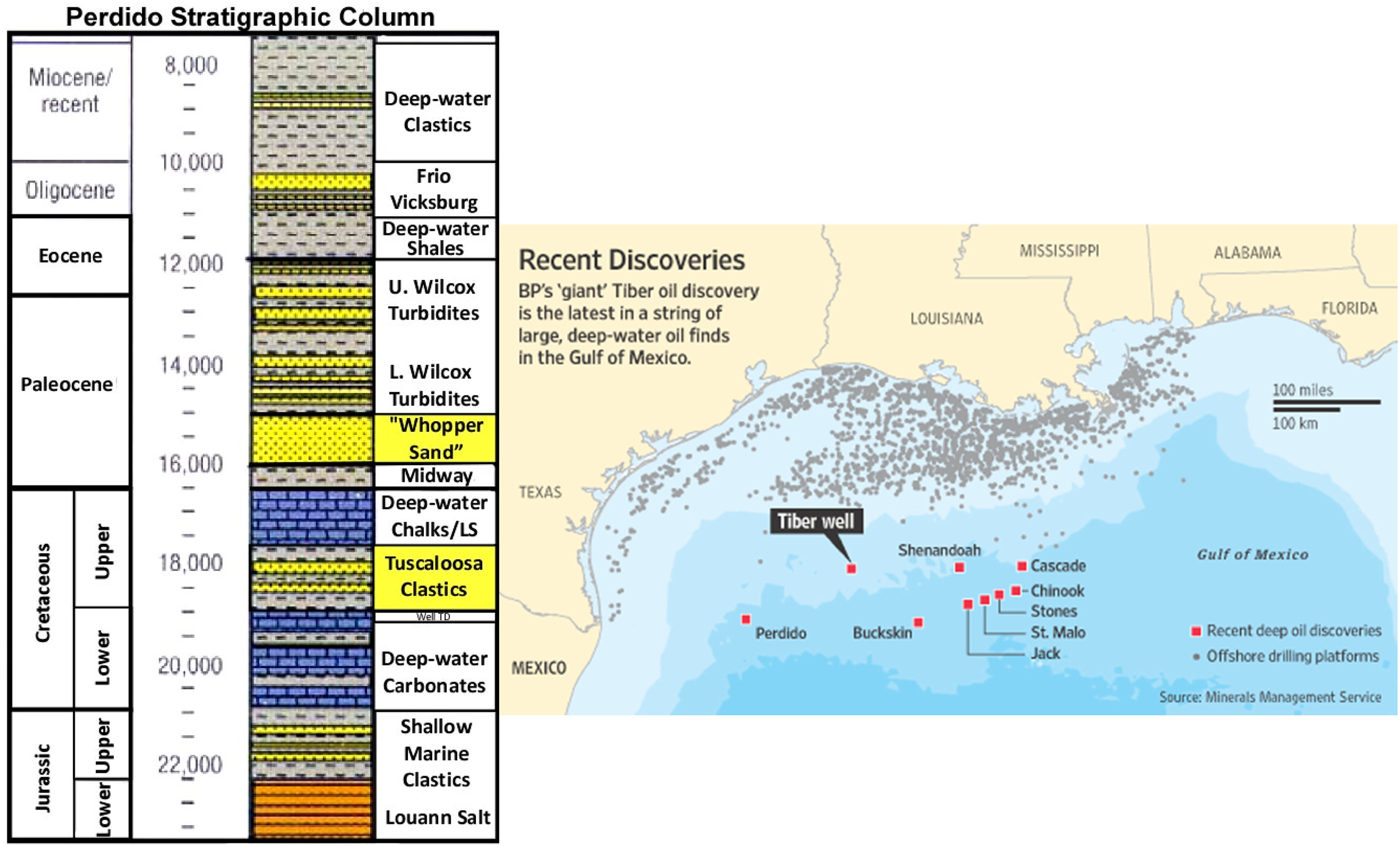
Lithological column (taken from Lach, 2010) and oil fields map (taken from Gold, 2009) of the Deepwater Gulf of Mexico.
Statistics of Paleogene fields in deepwater.
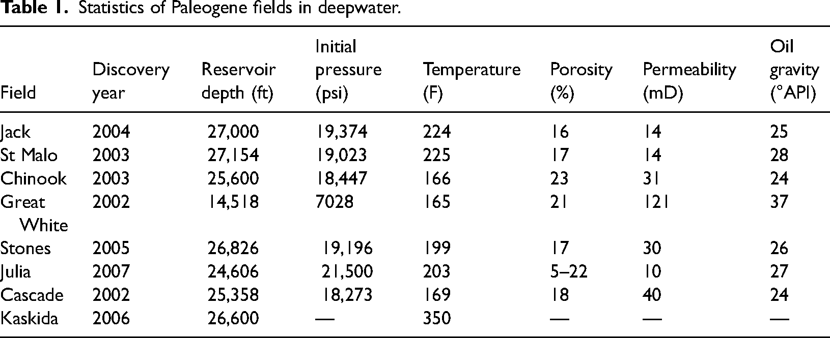
Hydrocarbon fluid properties are summarized from available publications. The wt% of sulfur varies from 0.5 to 3 and the gas-oil ratio varies from 300 to 2400 GOR (Lach, 2010), oil gravity varies from 22 to 41 API, and viscosity varies from 1 to 11 cP for lower oil viscosities, and 5–26 cP, for higher oil viscosities in over-pressurized formations. For over-pressurized reservoirs, pressure is higher than bubble-point pressure and the oil is initially undersaturated. Due to the lack of free gas, initial depletion is supported by the aquifer or fluid expansion, and after reaching to bubble-point pressure, solution gas drive becomes the main supportive energy if the aquifer is not large enough. High over-pressure and temperature are typical characteristics of Paleogene reservoirs in the Wilcox formation. For these reservoirs, initial pressure is higher, for example, at Jack and St Malo, the pressure and temperature are greater than 19,000 psi and 225 °F, respectively, and Kaskida and Tiber report temperatures greater than 300 °F (Lach, 2010).
Statistical analysis and summarization of the available data
After the compilation of the publicly available analog data (Bureau of Safety and Environmental Enforcement, 2011), data analytics is applied to calculate summarizations to condition numerical geostatistical reservoir models. Log measurements from fields Jack, St Malo, Stones, Anchor, Great White, and Whale are analyzed to calculate distributions of field predictor features, for example, porosity, permeability, and facies proportion. First, we show the distribution of these features for all six fields and then show detailed analytics of the Anchor field as an example to illustrate the methodology applied over all the fields.
Figure 2 includes the standardized distribution of neutron porosity, density, and NMR porosity for all six fields as a violin plot (a combination of boxplot and kernel density estimate, similar to box and whisker plot). Mean porosity measurements from neutron porosity are around 0.30 (Anchor-0.32, Stone-0.29, Whale-0.32, St Malo-0.25, Jack-0.28, Great White-0.28), although it is 0.15 for NMR porosity (Anchor-0.14, Stone-0.16, Whale-0.16, St Malo-0.16, Jack-0.18, Great White-0.17). NMR measurements are quite close to the average Wilcox formation porosity found in the literature. The average density value is approximately 2.45 g/cm3 for all fields.
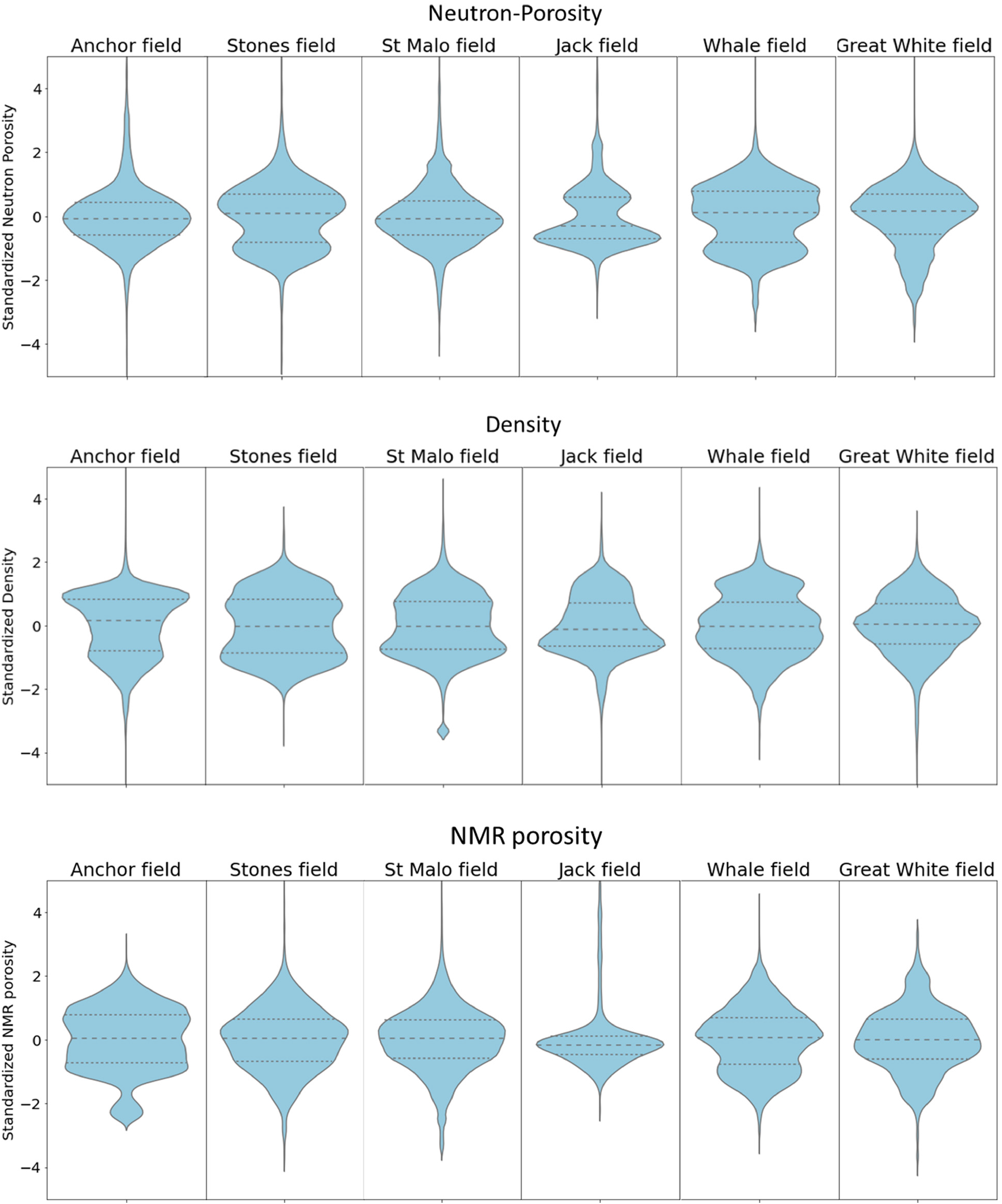
Violin plot of neutron porosity, density, and NMR porosity for six fields in the Wilcox formation.
Figure 3 is the matrix scatter plot to visualize the bivariate distributions and pairwise relationships of the four porosity-related log measurements for the Anchor field, including gamma ray (GR), neutron porosity (NEU), density (DEN), and nuclear magnetic resonance porosity (NMR). Similar univariate and bivariate distribution trends are observed Anchor field, and the arithmetic averages of GR, NEU, DEN, and NMR are 67.5, 0.29, 2.45, and 0.14, respectively. The standard deviation of GR, NEU, DEN, and NMR in the Anchor field is 14.3, 0.03, 0.11, and 0.06, respectively.
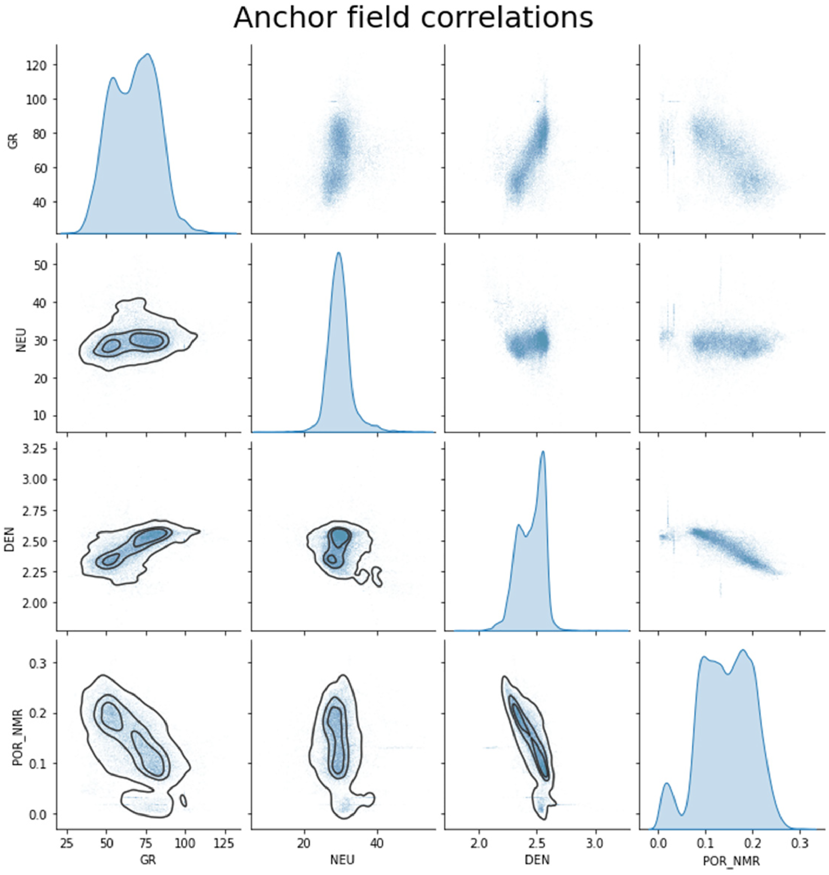
Pairwise correlation plot of gamma ray (GR), neutron porosity (NEU), density (DEN), and nuclear magnetic resonance porosity (POR_NMR) for anchor field.
To explore the univariate feature distributions between individual wells, Figure 4 includes the by-well violin plots for five wells of the Anchor field for neutron porosity, gamma ray, density, and nuclear magnetic resonance porosity. Gamma ray distribution is relatively consistent across five wells and unique for one of the wells, which may indicate geological trends. The reservoir unit thickness varies between 300 and 600 ft interpreted from gamma ray measurements. NMR porosity is consistent between the five wells with an average porosity of approximately 0.14 for each well. Similar to the field-wide distribution, neutron porosity values are higher than NMR which is also consistent among wells and is approximately 0.29.
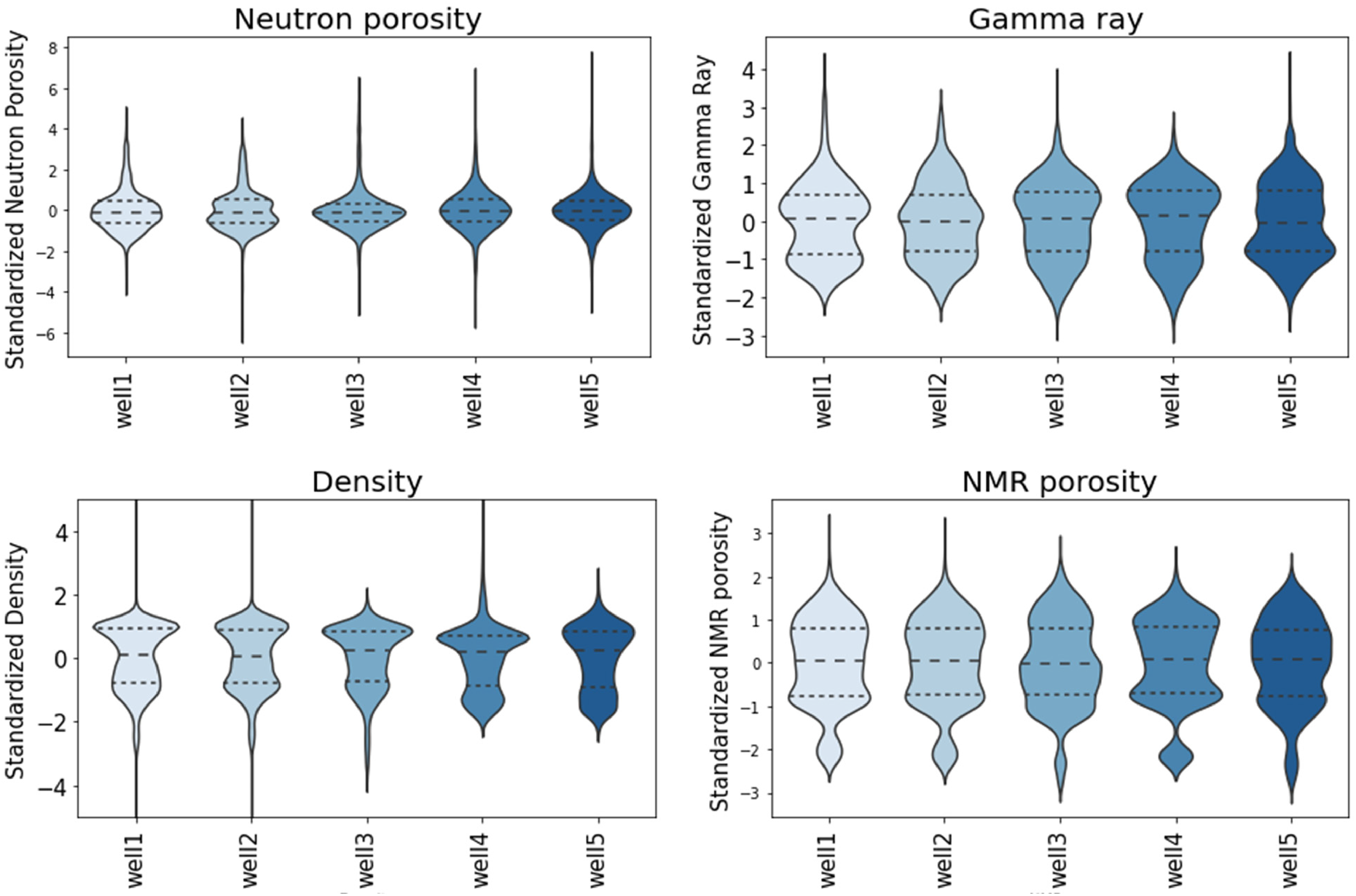
Violin plot of neutron porosity, gamma ray, density, and NMR porosity for five wells in the anchor field.
Base case model construction
The truncated Gaussian method is applied to build a sand and shale base facies model. This geostatistical method calculates categorical facies, sand, and shale, realizations by truncating a continuous, spatially correlated Gaussian random field with zero mean and unit variance. Directional spatial continuity based on a covariance function (variogram model) characterizes spatial correlation anisotropy with a range of 3000 ft in the dip and 1500 ft in the strike directions. The sand proportion is applied as a percentile to determine the Gaussian value to truncate the continuous Gaussian random field. Porosity is distributed within facies with Sequential Gaussian Simulation. We use a cookie-cutter approach to embed porosity distribution into the associated facies model. Permeability is generated using cloud transformation to ensure the reproduction of the bivariate relation between log permeability and porosity observed from core measurements within each facies. The base case model is geostatistically straightforward and provides a reasonable geological model given the large interval, space, and time of this analysis.
The base case grid model is constructed with the approximate expected values from the analyzed Paleogene GOM fields. The field model has an areal extent of 15,000 ft × 15,000 ft, with lower and upper units each with 500 ft thickness, separated by a 350 ft continuous, impermeable shale layer, and the grid structure is uniform thickness with a dip is 20°. The number of grid cells in the x and y directions is 50 and 101 in the z direction, which includes 50 cells for each reservoir unit and 1 for the shale layer. The regular grid cell size is 300 ft in the x and y areal direction and 10 ft in the z vertical direction to ensure that heterogeneity is preserved in the model (Figure 5).
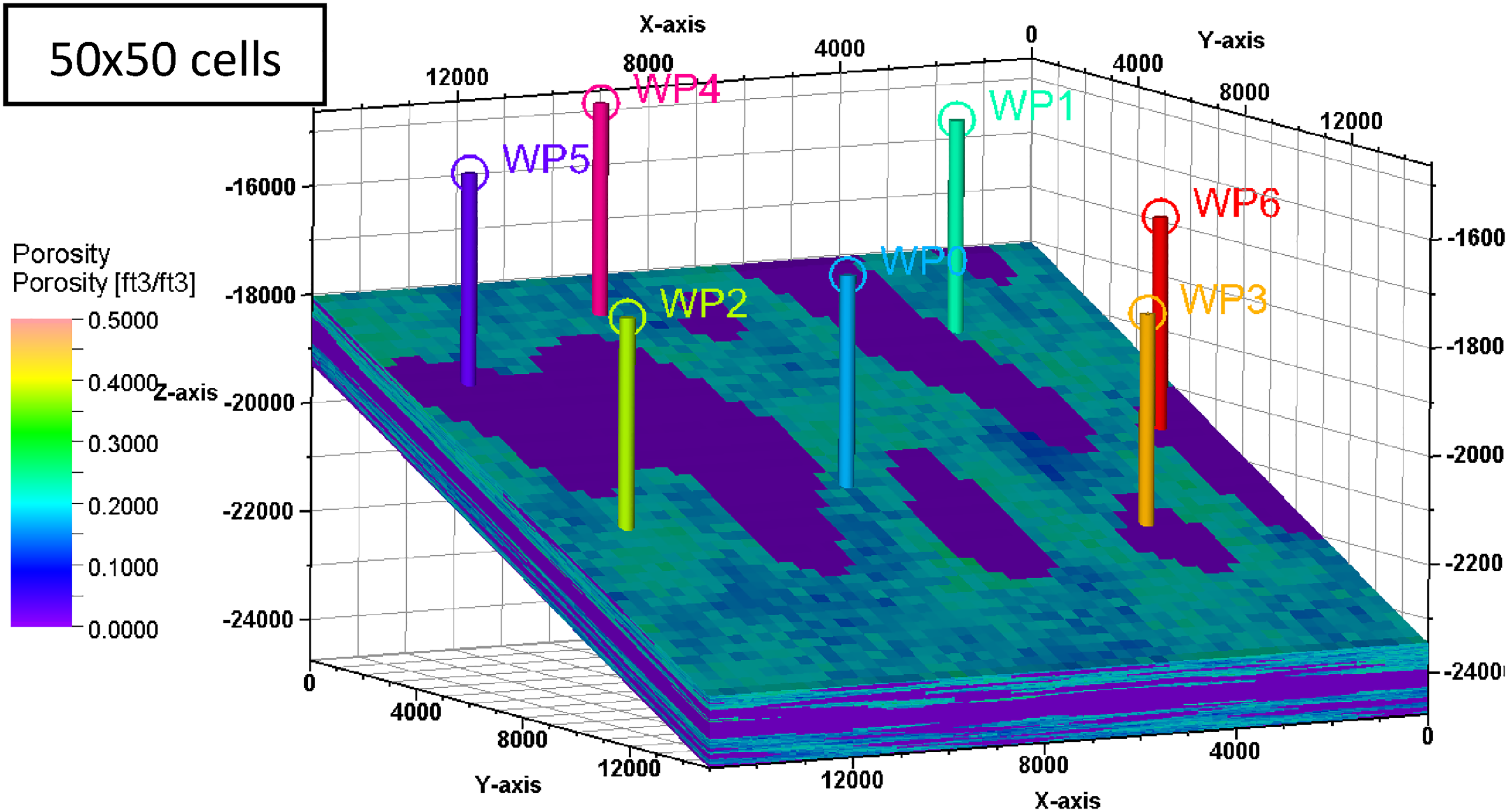
The static model with porosity distribution with seven production wells.
To test the sensitivity of grid size, both upscaled and downscaled versions of the static model were constructed, as shown in Figure 6. The downscaled model has 25-grid cells in both the x and y directions, each with a length of 600 ft, while the upscaled model has 100-grid cells in both directions with an extension of 150 ft. From the cumulative production curves presented in Figure 7, it is evident that the 25-grid cell model is too coarse and does not provide very accurate results. On the other hand, the 50- and 100-grid cell models produce comparable results for both production schemes. Therefore, to reduce computational run time, the 50-grid cell model is selected.
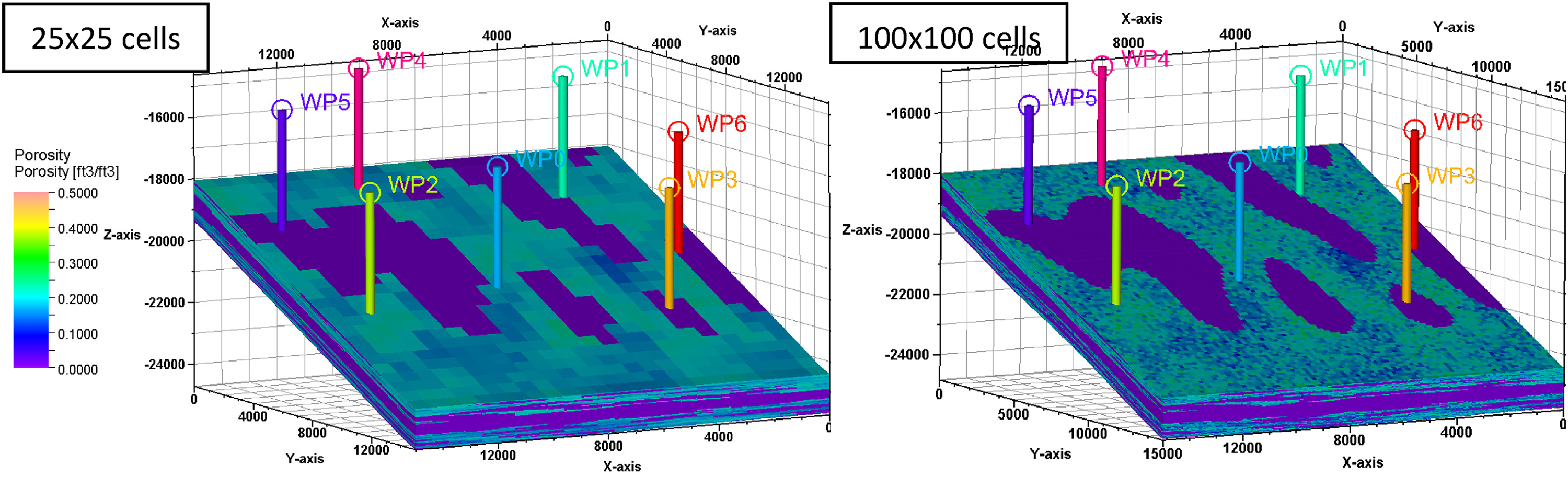
Upscaled and downscaled
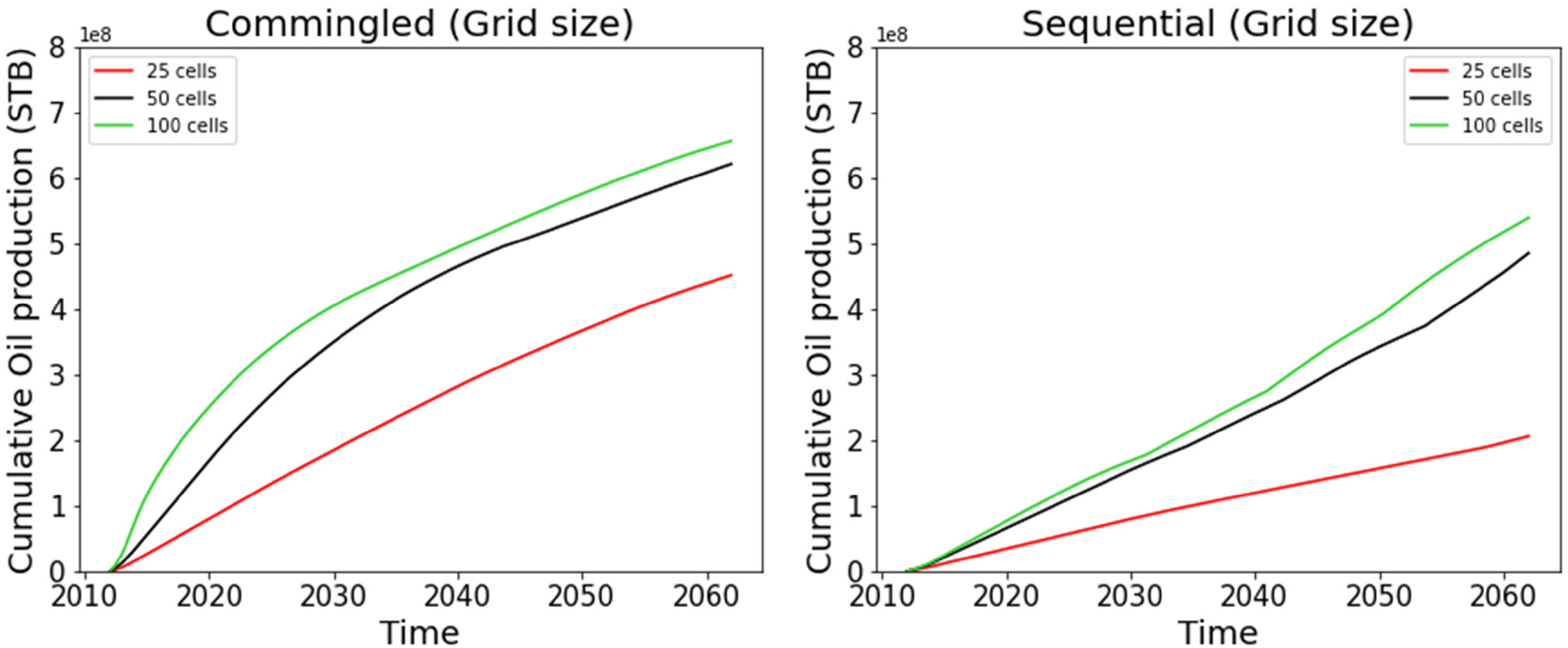
Cumulative production plots for commingled and sequential production schemes in grid size sensitivity.
The depth of the top of the reservoir is 18,000 ft, and the initial pressure is 18,000 psi at the datum depth of 21,000 ft. Average porosity values are 19% for upper and 17% for lower units and are distributed with 3% standard deviation. The permeability model is constrained by the bivariate relationship with porosity. The average permeability of upper and lower units is 20 and 10 mD, respectively. Permeability is distributed with 0.5 mD standard deviation.
After completing static model construction, the next step is dynamic simulation to forecast instantaneous and cumulative production rate, recovery, and crossflow between lower and upper pay units for primary pressure depletion production for both sequential and commingled production schemes. Existence of an aquifer five times larger than the reservoir makes the drive mechanism to be mainly water drive. Irreducible water and residual oil saturations are chosen to be 0.3 and 0.3, respectively. Oil–water relative permeability curve is shown in Figure 8.
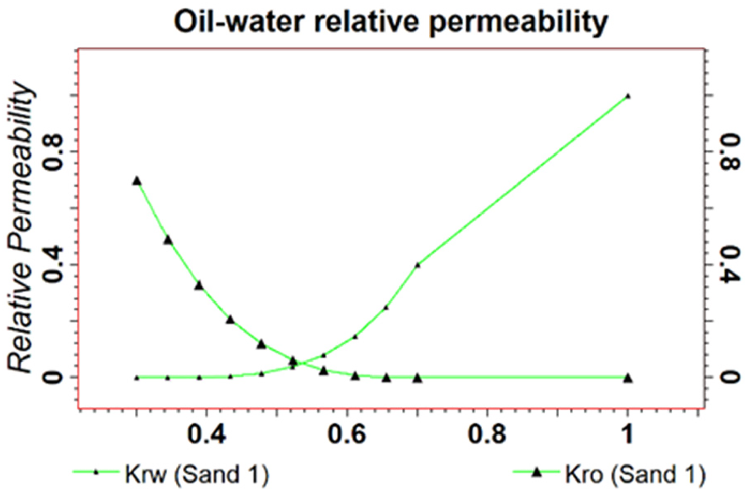
Oil–water relative permeability.
Production is controlled by seven vertical wells that are completed in both reservoir units with an approximately 4100 ft well spacing. Each well has two 150 ft completions separated by 100 ft in each pay unit (i.e., 150 ft completion followed by 100 ft separation, then 150 ft completion followed by 100 ft separation). Wells are controlled by the initial production rate and then switch to tubing head pressure control with a target of 400 psi.
All wells for the commingled production scheme start producing from upper and lower units at the start of the simulation. For sequential completion, wells start production from the lower unit and switch to the upper unit production when the production rate reaches the minimum allowable value of 800 STB/day. The sensitivity results on switching flowrate value from lower unit to upper unit are given in Figure 9. The tests are conducted by varying the flow rate from the lowest 600 STB/day to the highest 1500 STB/day. According to Figure 9, total production values at the end of 50 years for all six cases are approximately the same. However, selecting a flow rate value of 1500 STB/day may lead to leaving more oil in the lower unit, as it is an excessively high production value. Therefore, for economically feasible results, 800 STB/day is selected.
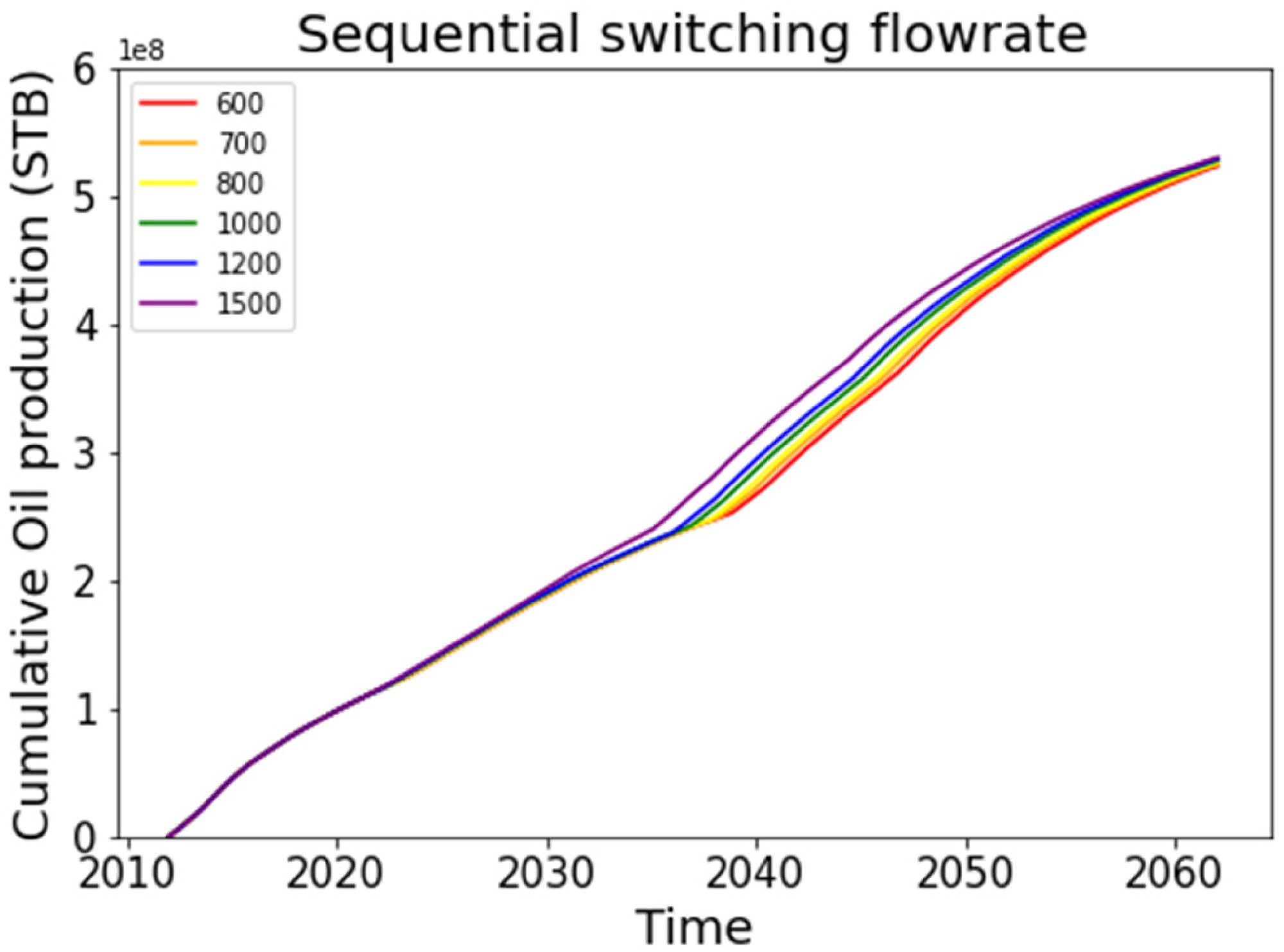
Cumulative production plots for sensitivity on switching flowrate of sequential production scheme from lower unit to upper unit.
Although 30 years of production time is more realistic, the forecast is calculated over 50 years for a fair comparison of sequential and commingled production schemes. We chose 50 years because the reservoir is very tight, and it may require a long simulation time for sequential production scheme wells to complete production from the lower unit and switch to the upper unit and then deplete it. However, we also show that commingling production scheme result in much higher oil recovery than sequential production scheme for a realistic scenario of 30 years.
Sensitivity analysis is applied to this base case model with a OFAT DOE based on a three-level design, base, high, and low case values for each of the 19 predictor features. While this design does not consider interactions, it does provide a practical design size given the number of field parameters and modeling and forecasting run times. To check for crossflow for the commingled production scheme between reservoir units, wells are randomly shut-in for a year and the difference between oil-in-place in each reservoir unit is calculated.
Results
This section provides the results of OFAT DOE sensitivity analysis over the 19 reservoir parameters using dynamic reservoir simulation for both the commingled and sequential production schemes.
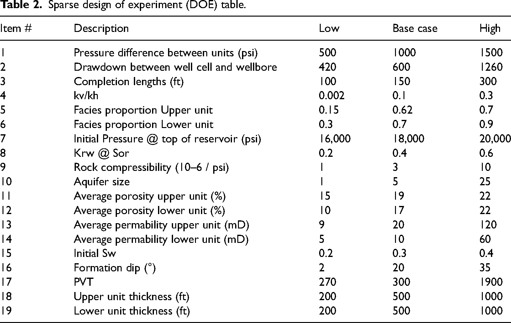
In Table 2, the column “Base case” contains the selected parameters for our reservoir simulation. The average porosity for upper and lower units is 19% and 17%, respectively, with 3% standard deviation which is determined based on NMR porosity log measurements of the six analog fields. From gamma ray measurements, we observe two reservoir units separated by a thick shale bed. Based on the initial pressure values given in Table 1, we have set 1800 psi at 21,400 ft depth (top of the reservoir) initial pressure for our base case model. As mentioned in the introduction, the average permeability distribution is between 10 and 30 mD for the Wilcox formation. Since reservoir quality in the lower unit is generally less than the upper unit, we choose an average permeability of 20 mD for upper unit and 10 mD for lower unit with a standard deviation of 0.5 mD.
Sparse design of experiment (DOE) table.
The cumulative oil production from the numerical reservoir simulation OFAT DOE is summarized in the tornado chart in Figure 10. The top five big hitters for the commingled production scheme are upper unit thickness, lower unit thickness, facies proportion of upper and lower unit, and rock compressibility. However, for the sequential production scheme, the top five big hitters are average permeability of lower unit, thickness of upper unit, facies proportion of upper and lower unit, and rock compressibility.
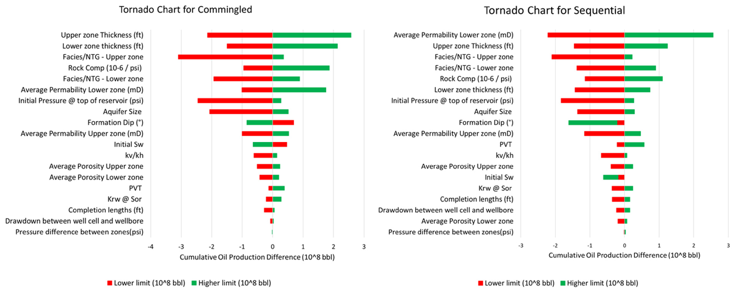
Tornado chart of commingle (left) and sequential (right) cumulative oil production for 50 years.
The tornado chart in Figure 11 shows the difference between total production for the commingled and sequential production schemes (commingled production minus sequential production) for 30 and 50 years of production. For 50 years of production, the commingled production scheme outperforms the sequential production scheme for all cases in the DOE. Note, in the case where the facies proportion of the upper unit is small, for 50 years of production, the difference between commingled and sequential production schemes is small. The only case where the sequential production scheme outperforms is for 30 years production period where the average permeability of lower unit is very high. Yet this difference between commingled and sequential production schemes is quite close to zero and may not be significant. This result is due to the sequential production scheme achieving full depletion of both units by switching to upper unit production in just 10–15 years after a rapid depletion of high-permeability lower unit (Figure 12). High cases for features such as PVT, initial water saturation, and average permeability of lower unit result in reduced production difference between commingled and sequential production. In these cases, as total productions from both completion techniques are closer to each other, the selection of production scheme should consider other parameters like production period, operational constraints on completion design, and other expert knowledge. The rest of the parameters indicate that the commingled production scheme results in significantly higher total oil production than the sequential production scheme.
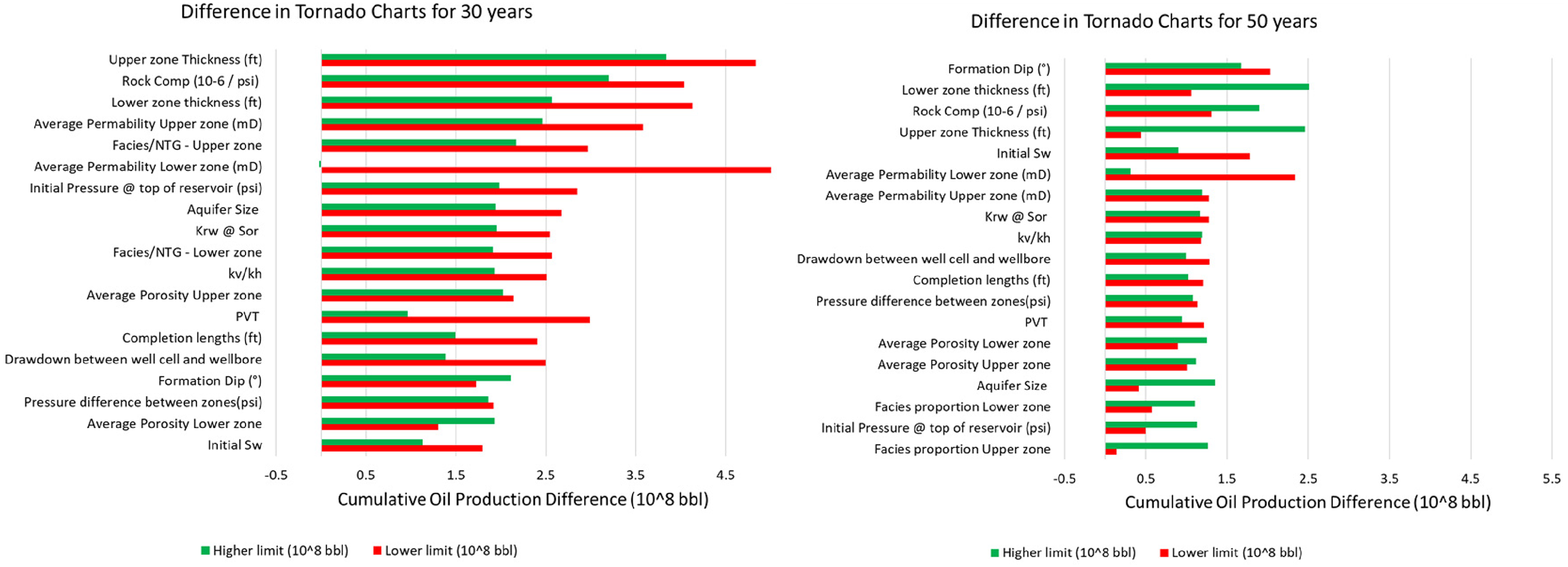
Tornado chart for the difference between commingled and sequential cumulative production values at the end of 30 (left) and 50 (right) years.
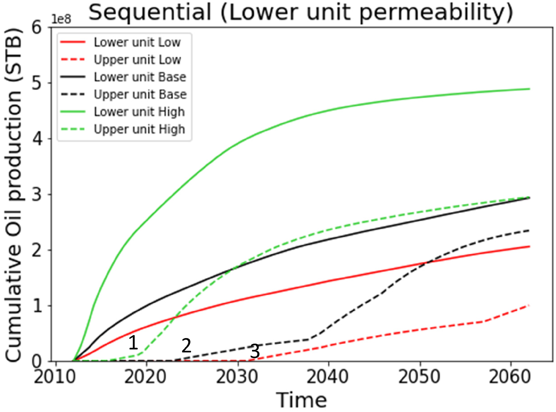
Cumulative production for sensitivity with high case of lower reservoir unit permeability value for 50 years sequential production scheme. (the times when the first wells switch production from lower unit to upper unit is indicated with numbers 1, 2, and 3 for low, base, and high cases, respectively).
Figure 13 includes cumulative oil production plots for both commingled (on the left) and sequential (on the right) production schemes for the top three field parameters (top three big hitters). Over long-term production, the highest production is achieved with static properties of the reservoir such as thickness of upper and lower units, or facies proportion of upper unit. Additional to these features, lower unit permeability is the most important parameter for sequential production scheme, which is extensively discussed in the preceding paragraph. As upper unit thickness increases to 1000 ft, total production increases by 41% for the commingled production scheme and 26% for the sequential production scheme (Figure 13). The second most important field feature is upper unit facies proportion for both production schemes. More sand proportion in the reservoir results in higher production. Commingled and sequential production increases by 7% and 6%, respectively, when the facies proportion of upper unit is increased to 0.7 from 0.62 and decreases by 48% and 67% when the facies proportion of upper unit is decreased by almost four times (Figure 13). The parameter with the least significant effect on production recovery for both commingled and sequential systems is the pressure difference between units. In both production methods, the total production and pressure curves are nearly identical (Figures 13 and 14).
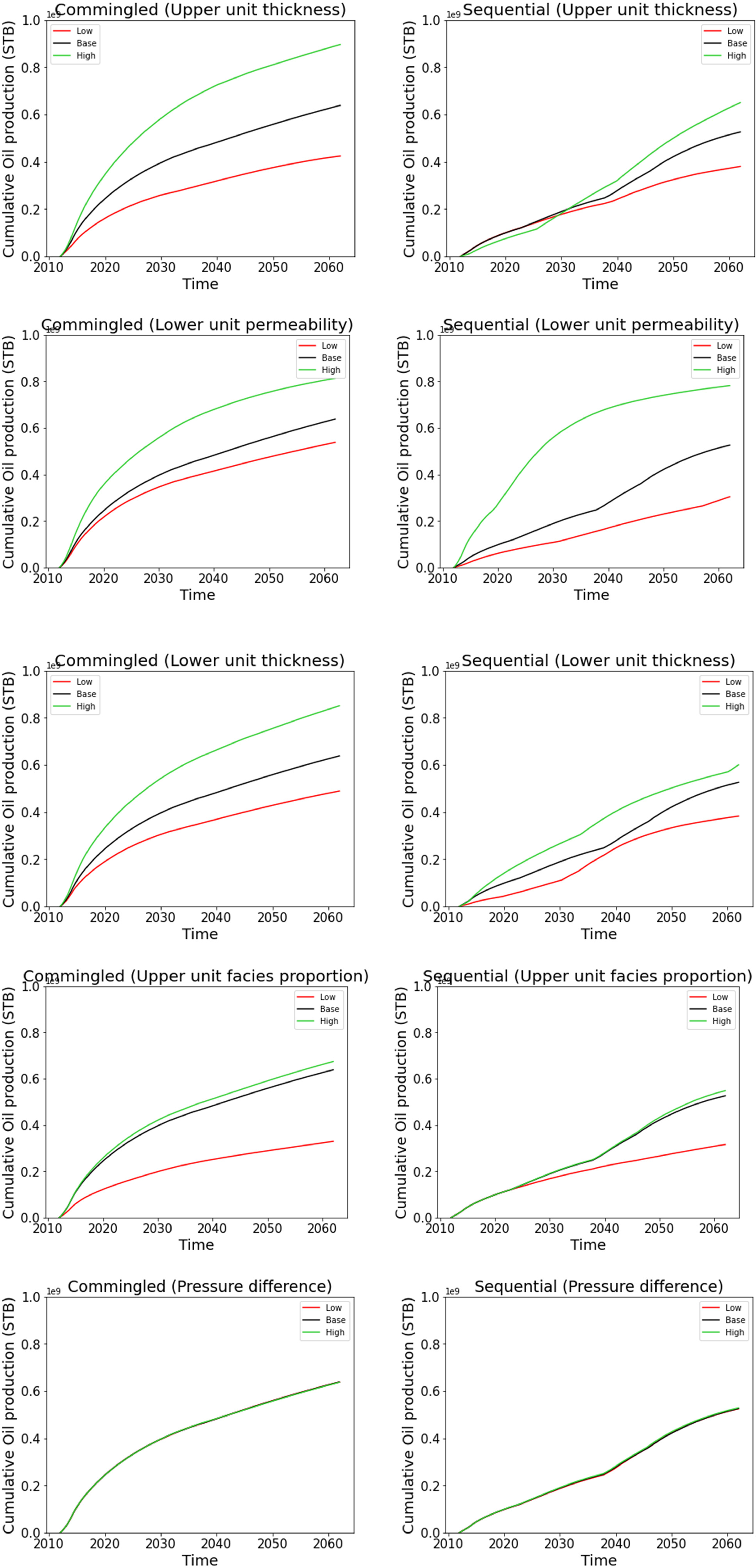
Cumulative production over 50 years for commingled (left) and sequential (right) production scheme for top three hitters it is shown in the first four pairs of plots. The last pair of plots shows the least important parameter which is pressure difference between reservoir units.
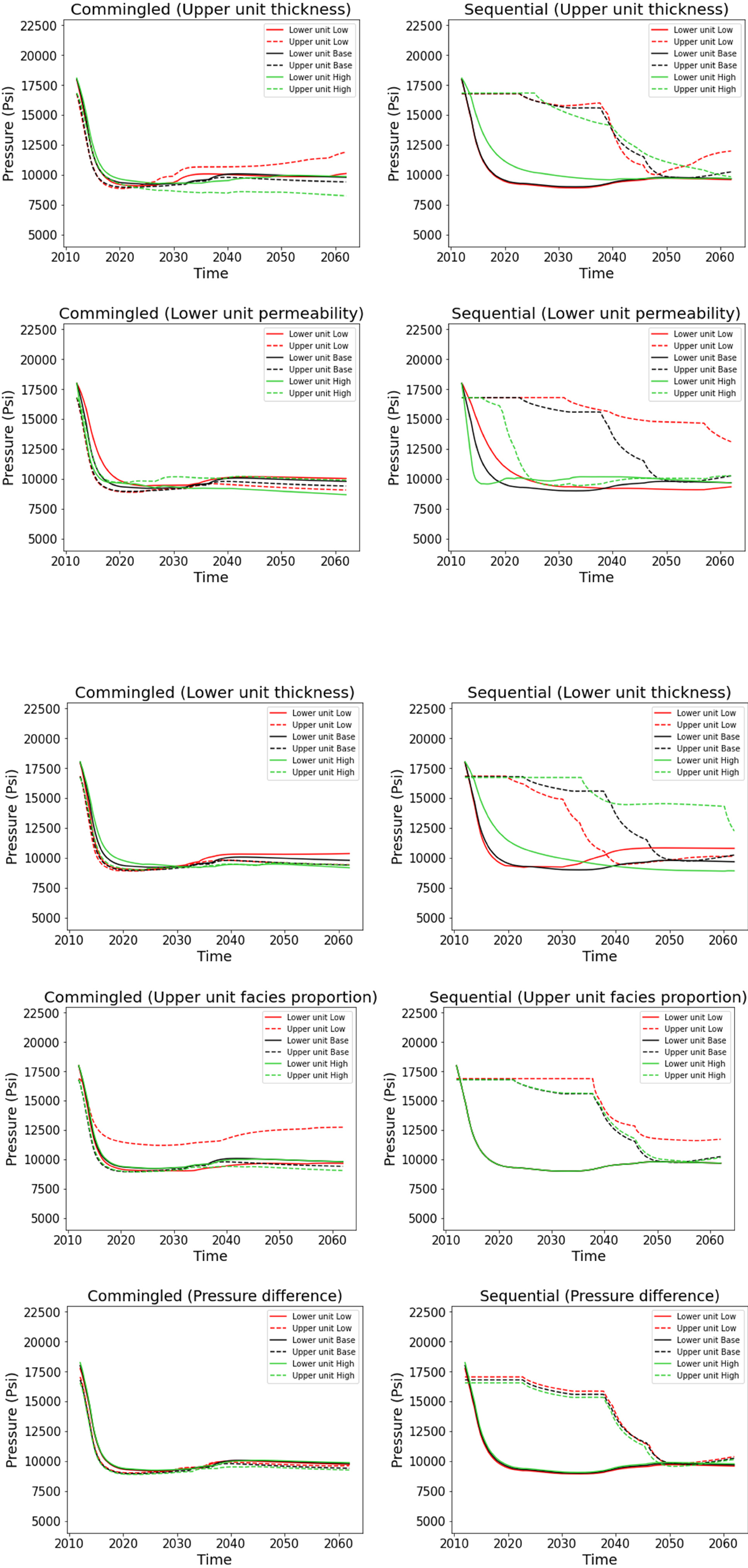
Field pressure plots over 50 years for commingled (left) and sequential (right) production scheme for top three hitters are shown in the first four pairs of plots. The last pair of plots shows the least important parameter which is pressure difference between reservoir units. For the sequential production scheme during the initial time period lower unit (solid black, red, and green lines), pressure starts decreasing. After a certain production period, as wells shut-off production from lower unit and start switching production to upper unit (dashed black, red, and green lines), upper unit pressure starts declining.
For the high case unit thickness, the reservoir pressure is preserved for a longer time (Figure 14). As for the previous initial pressure plots, pressure decline is steeper when we have small high permeability, which results in shorter earlier reservoir depletion. For the large low unit thicknesses, after approximately 20–30 years of production, we observe pressure build up in both commingled and sequential schemes. In the 2030s four out of seven wells result in water breakthrough and shut-in of premature wells. The pressure measurements shown in the graph are hydrocarbon pore-volume weighted-average pressure, and as production from four wells stops, the aquifer level increases and pushes the hydrocarbons upwards. As a result, we observe a slight increase in pressure and production rate for the three remaining wells (Figures 13 and 14).
From cumulative water production tornado charts for commingled and sequential production schemes (Figure 15), the average permeability of lower and upper units is the most important predictor features for both production schemes. Aquifer size is among the most impactful feature of both production schemes. As aquifer size increases, not only pressure support and cumulative oil production increase, but also higher water production is observed. The effect of the remaining parameters is significantly less on water production.
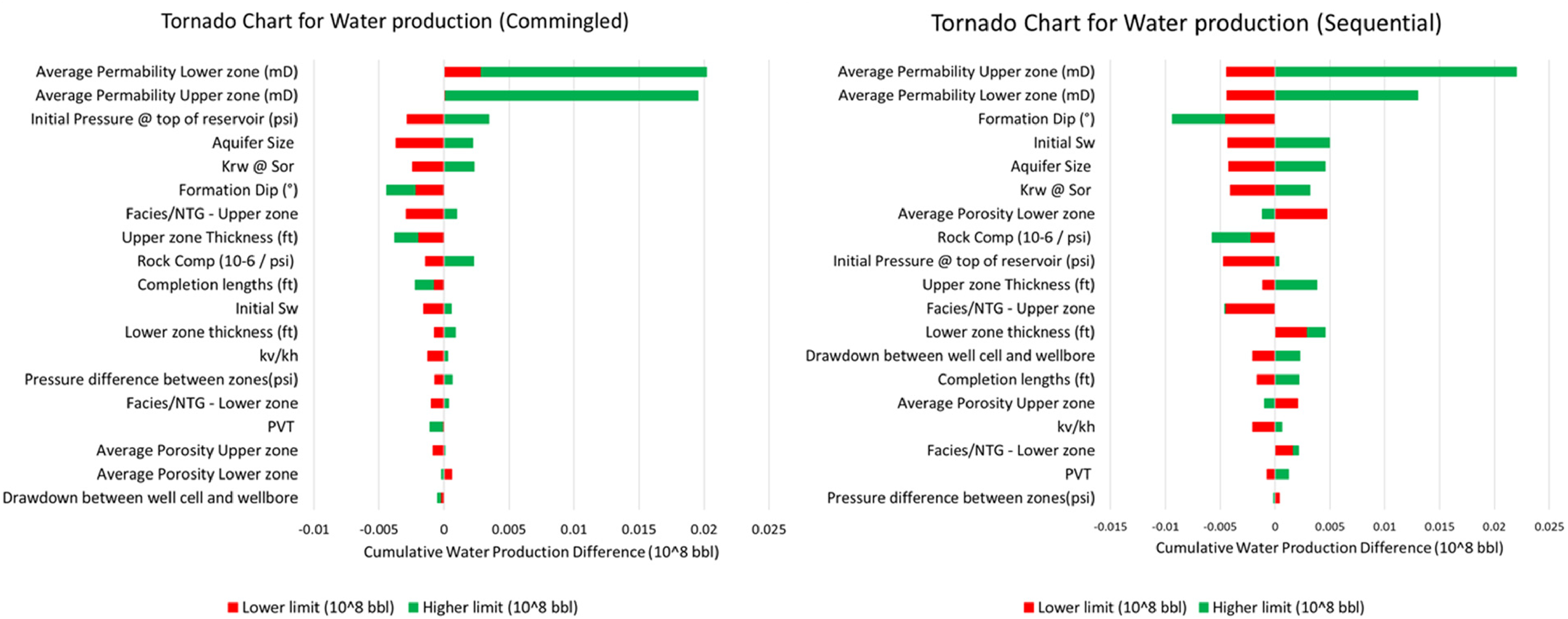
Tornado chart of commingle (left) and sequential (right) cumulative water production for 50 years.
Discussion
In this section of the paper, we extend the findings from the previous section and examine the impact of crossflow and spatial uncertainty on production in both commingled and sequential production schemes.
Crossflow test
One of the main disadvantages of a commingled production scheme is crossflow as previously mentioned. To check the amount of fluid flowing between Lower and Upper Wilcox, we shut-in all seven wells simultaneously for 1 year and measure the flow rate and total volume of fluid flow from one unit to another. From the crossflow tornado chart (Figure 16), reservoir-rock quality properties such as permeability of upper and lower units, net-to-gross, rock compressibility, and aquifer size are the most impactful predictor features. To highlight the volume of crossflow, percentage values of the crossflow volume relative to cumulative oil production are included in Figure 16. Most cases have a percentage lower than 1.5% indicating the crossflow volume for the commingled production scheme is negligible.
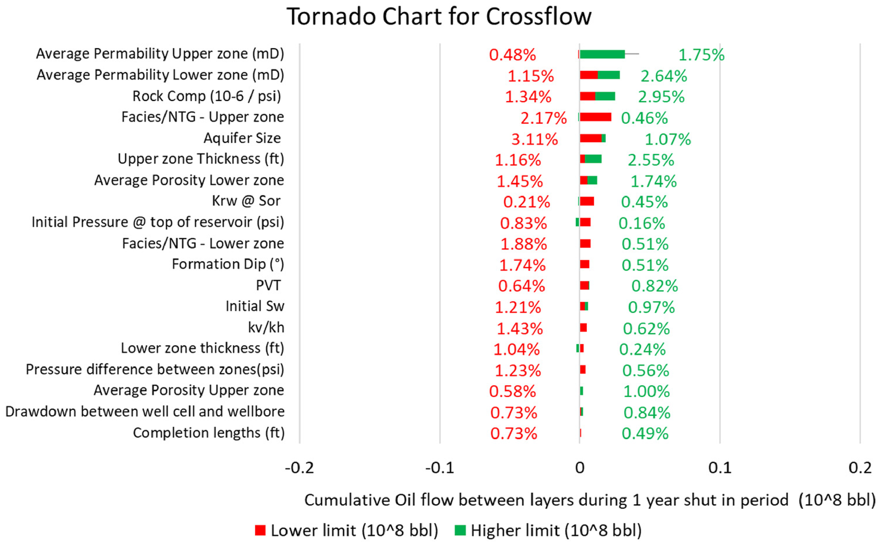
Tornado chart with 1-year long crossflow shut-in for commingled production scheme.
To put this in perspective, we calculate the synthetic repeat formation tester pressure and flowrate for each well completion to evaluate high-resolution flow between the well bore and formation within the Lower and Upper Wilcox units. For the indicated most impactful predictor features, the high resolution along well pressure differences, and direction and amount of flow are shown (Figures 17–19). In the flowrate plots, we have both positive and negative flowrate values, where positive indicates fluid flows from the reservoir into tubing in that grid cell, and negative indicates fluid enters the reservoir. Pressure plots demonstrate that lower unit pressure is higher than upper unit. As fluid flows from high pressure to low pressure, we observe positive flowrate in lower unit cells and negative flowrate in upper unit cells. There are some exceptions such as wells 3, 4, and 6. There is crossflow both within one unit and across units. This indicates that a sequential production scheme can also suffer from crossflow within one reservoir unit. To conclude, we can summarize that volume and flowrate of fluid flowing from one unit to another is not significant relative to the total production rate.
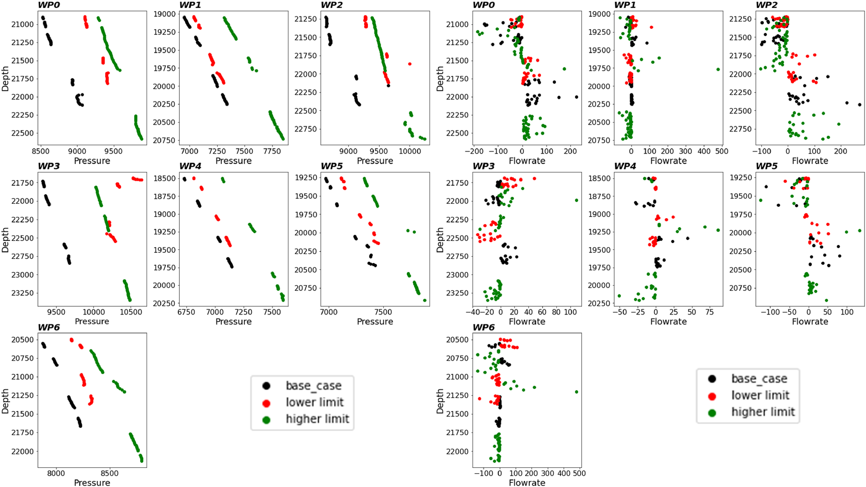
Repeat formation tester (RFT) (left) & flowrate (right) for upper unit thickness.
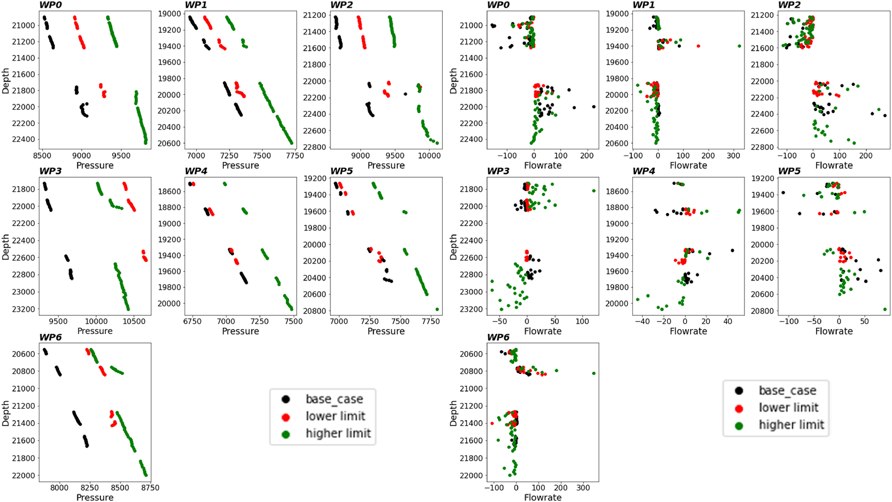
Repeat formation tester (RFT) (left) & flowrate (right) for lower unit thickness.
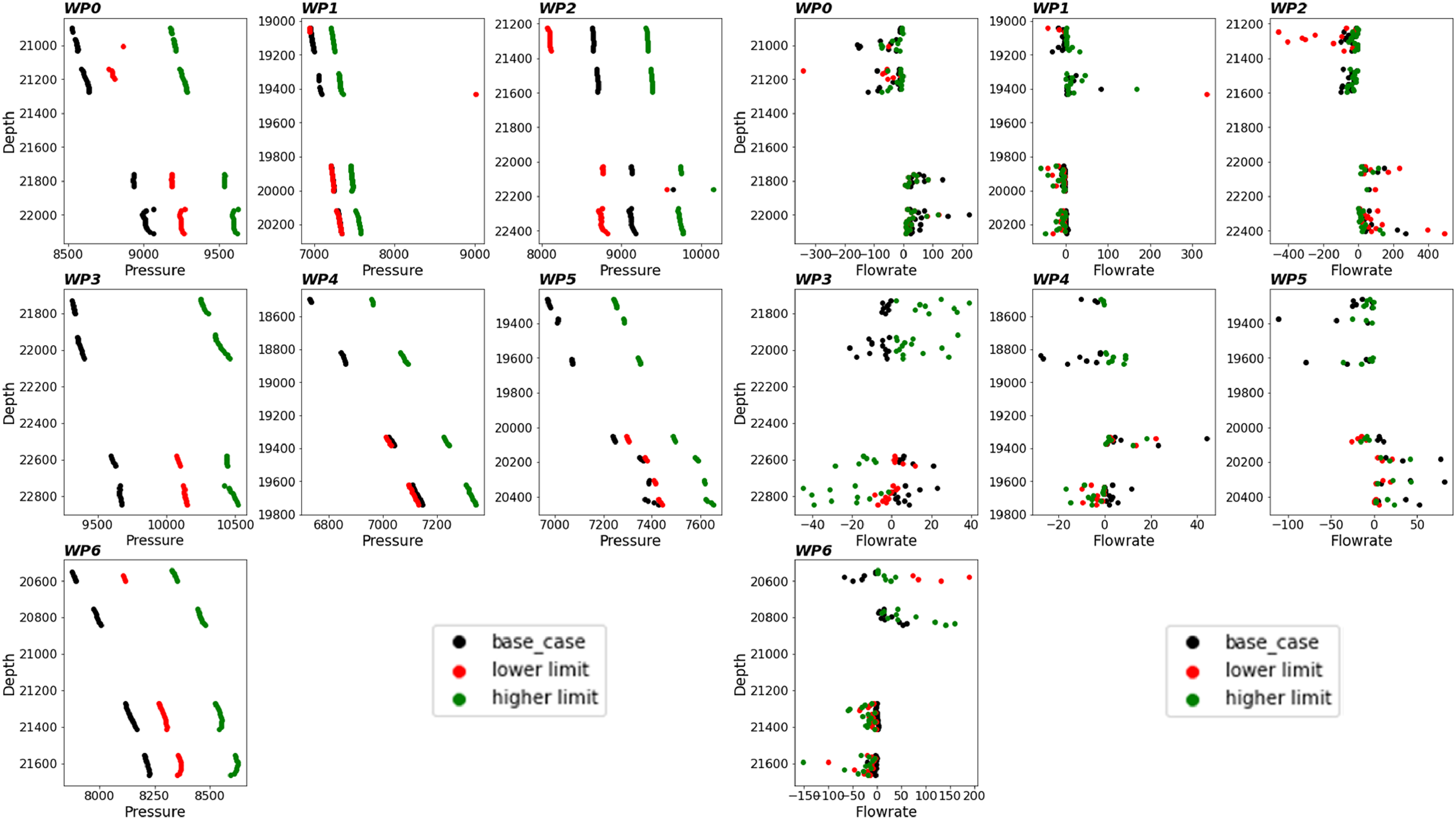
Repeat formation tester (RFT) (left) & flowrate (right) for facies proportion of upper unit.
Spatial uncertainty test
The previous DOEs with by-well and by-field scales provide replicates to observe the results over various well and reservoir configurations. To check for spatial uncertainty and to provide more confidence in our conclusion, we calculate five reservoir model realizations (Figure 20
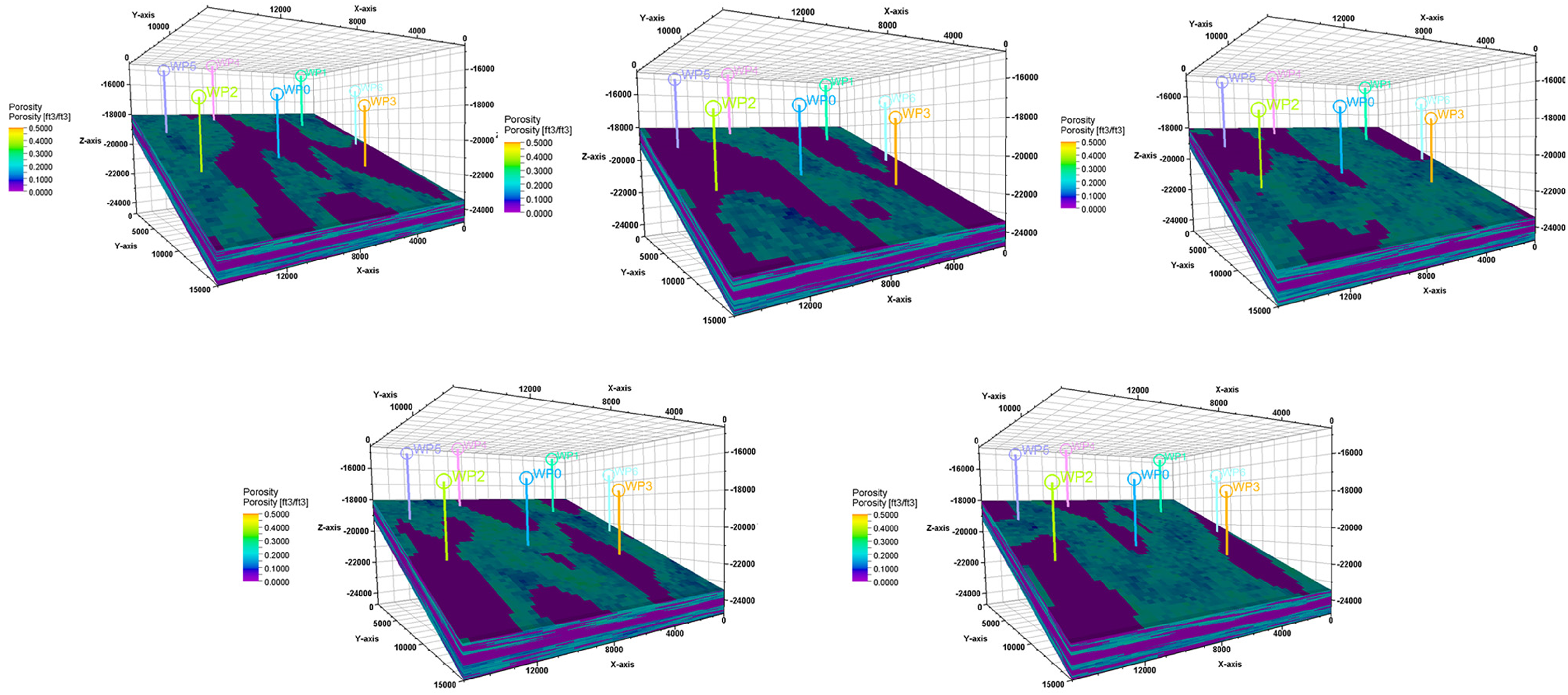
Five stochastic reservoir realizations.
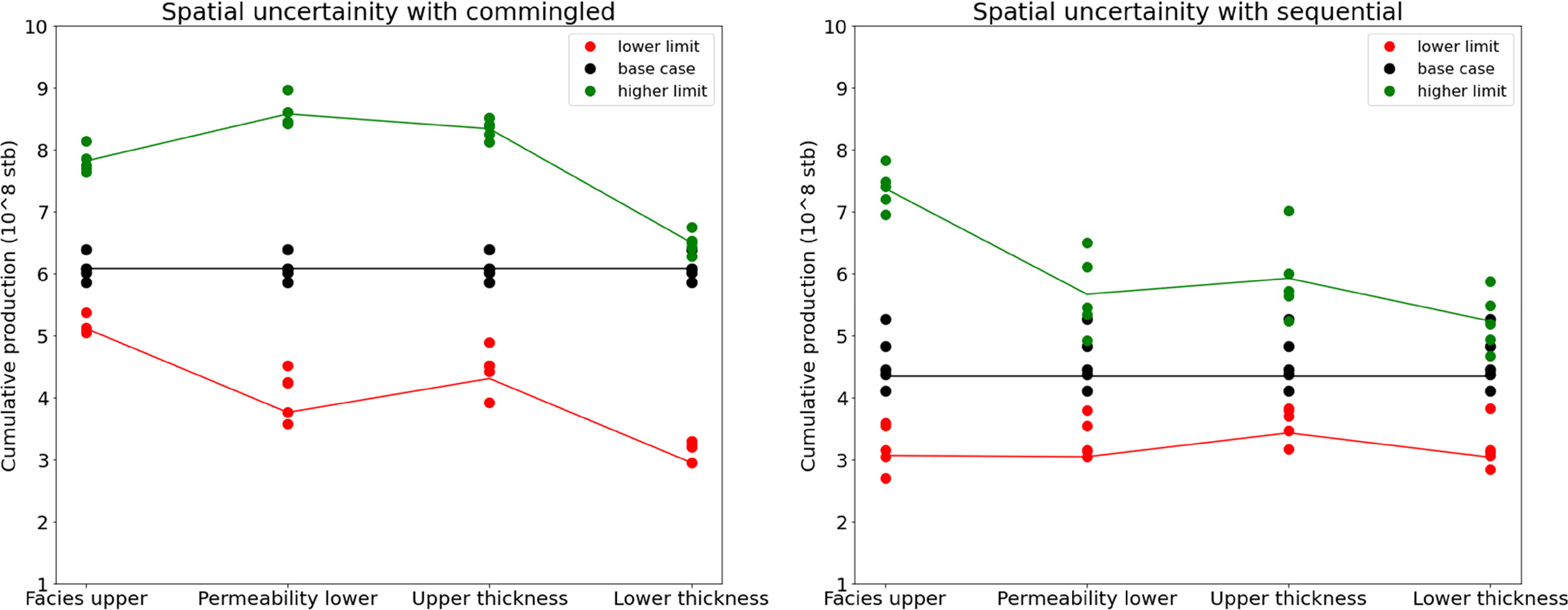
Cumulative productions from five different realizations for three big hitter parameters (commingled scheme on the left & sequential scheme on the right) and expectation lines.
Conclusion
We conduct a OFAT sensitivity analysis to compare commingled and sequential production schemes for Paleogene deepwater turbidite fields in the Central Gulf of Mexico. The DOE table includes 19 reservoir parameters in low, base, and high cases. Commingled production consistently yields oil recovery higher than sequential production. Production and pressure behaviors for the top three hitters are analyzed for both production schemes. The crucial factors influencing oil recovery for both schemes are upper and lower units’ thicknesses, facies proportion, and lower unit average permeability, as revealed by the OFAT DOE sensitivity analysis. Numerical simulation results spanning 30 and 50 years further confirm the superior performance of commingled production in both short and long term, achieving 61% higher oil recovery over 30 years and 21% higher over 50 years. Crossflow between Lower and Upper Wilcox units is examined for the commingled scheme, showing no significant impact on total production. Similarly, the results show that fluid flow within the same unit can be observed for the sequential production scheme. To validate our base case static model and address spatial uncertainty, we create five reservoir model realizations. Cumulative production is similar among the five realizations for the commingled production scheme and only slightly varies for the sequential production scheme. This reinforces the reliability of our simple but reasonable geological base case model. Future work will involve a more comprehensive study using advanced geological models to explore additional geological features.
Footnotes
Declaration of conflicting interests
The author(s) declared no potential conflicts of interest with respect to the research, authorship, and/or publication of this article.
Funding
The author(s) disclosed receipt of the following financial support for the research, authorship, and/or publication of this article: The authors express their gratitude for the support received from the Digital Reservoir Characterization Technology (DIRECT) Industry Affiliate Program at the University of Texas at Austin.