Sage Journals: Discover world-class research

Abstract

ROP (Rate of Penetration) is a comprehensive indicator of the rock drilling process and how efficiently predicting drilling rates is important to optimize resource allocation, reduce drilling costs and manage drilling hazards. However, the traditional model is difficult to consider the multiple factors, which makes the prediction accuracy difficult to meet the real drilling requirements. In order to provide efficient, accurate and comprehensive information for drilling operation decision-making, this study evaluated the applicability of four typical regression algorithms based on machine learning for predicting pore pressure in Troll West field, namely SVR (Support Vector Regression), Linear regression, Regression Tree and Gradient Boosting regression. These methods allow more parameters input. By comparing the prediction results of these typical regression algorithms based on R²(R-Square), explained variance, mean absolute error, mean squared error, median absolute error and other performance indicators, it was found that each method predicted different results, among which Gradient Boosting regression has the best results, their prediction accuracy is high and the error is very low. The prediction accuracy of these methods is positively correlated with the proportion of the training data set. With the increase of logging features, the prediction accuracy is gradually improved. In the prediction of adjacent wells, the ROP prediction methods can achieve a certain prediction effect, which shows that this method is suitable for ROP prediction in Troll West field.

Keywords

ROP machine learning real-time prediction regression algorithm algorithm comparison parameters combination analysis

Introduction

ROP has been a source of interest in drilling operation since the rate at which a well is drilled is a key indicator of the efficiency (Chiranth et al., 2017), which has an important influence on the well cost and safety. Accurate modeling of the relationship between mechanical drilling speed and influencing factors is essential to predict mechanical drilling speed and optimize engineering parameters. Proper ROP prediction is beneficial to a better understanding of the drilling status and thus contributes to reasonable drilling cost and risk control.

A variety of ROP models were proposed, researchers contributed to link the comprehensive relationship between ROP and weight on bit (WOB), rotational speed, tooth wear, pressure difference and hydraulic factors. Since the 1960s, researchers have already been working on the prediction of ROP. Maurer (1962) presented the ROP equation for the ideal bottom hole cleaning based on the cone bit. Later on, Galle and Woods (1963) proposed a prediction model of ROP considering bit weight, rotating speed, forming type and bit tooth wear. Then Mechem and Fullerton (1965) put forward a new model considering formation drilling capacity, bit weight, bit speed, well depth, mud pressure and hydraulic application. Bourgoyne and Young (1974) studied the effects of formation depth, strength and compaction, bottom hole pressure difference, bit diameter, bit weight, rotating speed, bit wear and hydraulic mechanics on drilling speed, and established a mathematical model to estimate drilling speed by multiple regression analysis. They also introduced the optimum value of the selection of the bit weight, the rotating speed, the hydraulic pressure of the bit and the technique of using the multiple regression method to calculate the formation pressure of the detailed drilling data. Tansev (1975) presents a new method for optimizing the life of ROP and bit and cost function based on the interaction of original data, regression and optimization methods. Some regression equations for predicting the life of ROP and bit are established by using the parameters such as bit speed, bit weight, hydraulic horsepower and so on. Al-Betairi et al. (1988) proposed a model to predict the influence of various drilling parameters on ROP by multiple regression analysis. The correlation coefficient and multiple collinearity sensitivity of drilling parameters were studied. Maidla and Ohara (1991) developed a computer software for optimizing the type of roller cone bit, bit speed, bit weight and bit wear to minimize the drilling cost per foot of a single bit. Hemphill and Clark (1994) considering the chemical properties of drilling mud, the effect of mud on ROP was studied by testing different types of PDC bit and drilling mud. Ritto et al. (2010) carried out robust optimization of drilling speed, and introduced a new method to optimize ROP, which is a function of drilling speed and initial reaction force of bit, vibration, stress and fatigue limit of power system. Alum and Egbon (2011) proposed an analytical model of ROP estimation based on the ROP estimation model proposed by Bourgoyne and Young. A series of studies have been carried out, and it is concluded that only the annular pressure loss has a significant effect on ROP through the equivalent cyclic density.

From the above studies, it can be seen that the classical method tends to concentrate on the factors affecting ROP, such as drilling pressure, rotational speed, drilling fluid performance, hydraulic parameters, formation characteristics, bottomhole pressure difference, bit working time and tooth wear, etc., and obtain the relevant drilling speed equation or function by analyzing the influence of individual factors on mechanical drilling speed. The factual situation is that there are many uncertainties in the drilling process, as well as complex coupling relationships between the various components, resulting in a large difference between the predicted and actual results of traditional methods.

In recent years, with the rapid development of artificial intelligence, various machine learning algorithms have been widely used in the field of petroleum engineering. For example, Farahani et al. (2018) developed a robust modeling approach to predict the shear stress for the thixotropic fluids as a function of the shear rate and the other parameters. Another example, Norouzi et al. (2019) applied a novel Hybrid Particle Swam Optimization-Simulated Annealing method (HPSOSA) to develop a new correlation to predict CO2-Oil minimum miscibility pressure (MMP). There are likewise many scholars who have made outstanding contributions in the area of ROP prediction. Hankins et al. (2015), by simulating the drilling operation of the old well in northwest Louisiana, predicted and optimized the operating parameters and equipment, optimized the drilling technology of bit weight, rotating speed, bit performance and hydraulic variables, and reduced the drilling cost to the lowest. Mostafa and Meysam (2016) used response Surface method and BAT algorithm to predict and optimize ROP. Chiranth et al. (2017) evaluated two different approaches to ROP prediction: physics-based and data-driven modeling approach, compared traditional models to data-driven models for ROP modeling and prediction. Turned out that data-driven models were more accurate in prediction of ROP in every formation that was tested. A new empirical correlation based on an optimized artificial neural network (ANN) model was developed to predict ROP alongside horizontal drilling of carbonate reservoirs as a function of drilling parameters, such as rotation speed, torque, and weight-on-bit, combined with conventional well logs, including gamma-ray, deep resistivity, and formation bulk density. Zhou et al. (2021) proposed an improved sliding window approach to update the prediction model by using mutual information analysis to determine appropriate model inputs and combining the K-nearest neighbor algorithm and dynamic time warping (KNN-DTW) to identify drilling conditions. An empirical equation for ROP estimation was developed (Al-AbdulJabbar et al., 2021) based on the optimized artificial neural network(ANN) model, and the predictability of the new ROP equation was compared with the existing correlation coefficients. Meanwhile, many scholars have also used machine learning algorithms for reservoir simulation studies in the field of oil and gas field development in recent years. Bhattacharyya et al. (2022a, 2022b, 2022c) developed a novel data-driven-based model that could accurately predict the decline curves and EUR (Estimated Ultimate Recovery) for new wells based on the data collected from nearby wells and this paper presented use of new algorithm as well as a new dataset. Bhattacharyya et al. (2022a, 2022b, 2022c) developed an innovative machine learning (ML) (random forest (RF)) based model for fast rate-decline and EUR prediction in Bakken Shale oil wells. Bhattacharyya et al. (2022a, 2022b, 2022c) presented a novel approach for reservoir simulation that used Random Forest (RF) which is one of the widely used Machine learning (ML) algorithm to reduce the number of iterations at each time step and speed up the simulation process. The study's novelty was in developing a new ML-based reservoir simulator that would make reservoir simulation much faster and computationally more efficient. In 2022, Bhattacharyya et al. optimized the model. They selected well parameters from publicly available databases of the Eagle Ford Shale formation Texas RRC (Railroad Commission of Texas) and employed Artificial Neural Network (ANN) to build Machine learning models as a function of the above well parameters for the corresponding model parameters as well as cross-validation technique such as k-fold cross validation to estimate the predictive accuracy of these models when applied to new or test wells.

The continuous development of monitoring technology during drilling process provides more and more valuable information for accurate prediction of ROP. However, conventional empirical or semi-theoretical models are normally under specific assumptions and fail to accommodate multiple parameters beyond their limitation. This makes it difficult for the classical models to consider the interaction of multiple factors in an all-round way, and thus cannot make full use of all the parameters measured while drilling. Developing intelligent model for ROP prediction would provide a new approach, which could utilize multiple factors. Some potential correlations, possibly ignored by classical assumptions, may be observed by the data-driven intelligent approach. In this paper, the effectiveness of typical machine learning algorithms, specifically the regression methods (SVR, linear regression, Elastic-Net regression and GBR algorithm) on ROP prediction are evaluated. Relevant Troll West field data from the literature (including up to 15 influencing factors) were used to train the model and methodological comparisons and parametric analyses were carried out. Data from adjacent wells were used to test the trained model and to verify the effectiveness of the applied algorithm and the combination of control parameters for ROP prediction.

In this paper, SVR, linear regression, GBR algorithm and regression tree methods are used to fit three sets of data. These methods allow more parameters input and are computationally fast, and higher accuracy of the GBR algorithm, which is critical for high-cost drilling jobs in the field. The method in this paper considers the input of 15 influence factors including depth, DHRPM, bending moment, bending RPM, caliper, density, torque, WOB, gamma ray, lateral vibration, near bit inclination, etc., simultaneously. Method comparison and parameter analysis are conducted to investigate the effectiveness of the method applied and the dominating parameter combination for ROP prediction. The Troll West oilfield data from the literature are used for the modeling study in this work. This method can predict the ROP in real time, provide the basis for safe and efficient drilling, and provide technical support for the development of smart drilling.

Methodology

The four basic models of machine learning are classification, clustering, dimensionality reduction and regression. Common regression algorithms include linear regression, support vector regression, gradient boosting regression, regression trees, random forest regression, and elastic network regression. In this section, the first four algorithms are selected as models for training. Linear regression is studied as the base model because it is fast and easy to model. Support vector regression has excellent generalization ability, is robust to outliers, and is valid in high-dimensional spaces for solving multi-factor problems. The overall process of regression trees is similar to that of classification trees, with branching exhausting every threshold for every feature without estimating values or removing missing records, and the regression trees can be improved and upgraded using the boosting framework in integrated learning. GBR, on the other hand, integrates many weaker models to form a more powerful learning algorithm and therefore fits better. In this section, the performance of these four methods is presented, as well as the parameters for evaluating the prediction performance, and the most advantageous method will be observed by comparing the evaluation results.

Introduction of regression algorithms

In this paper, four typical regression algorithms are selected to train the model and provide prediction results for the ROP, they are SVR, Linear regression, GBR algorithm and Regression tree method.

SVR.SVR (Support Vector Regression) is an important application branch of SVM (Support Vector Machine) (Nourali, 2019). SVR is to find a regression plane so that all the data of a set is the closest to the plane, even if the ‘distance’ to the farthest sample point of the hyperplane is the smallest. It transforms the actual problem into a high-dimensional feature space through a non-linear transformation, and constructs a linear decision function in the high-dimensional space to realize the non-linear decision function in the original space, which cleverly solves the dimensionality problem and ensures a good generalization capability, and the complexity of the algorithm is independent of the number of sample dimensions.

SVR regression prediction is based on the principle of correlation of prediction, and then find out the mathematical model between these characteristics and prediction targets. After the model is determined, the model is used to predict the change value of the feature. The hyperplane decision boundary in SVM is an SVR regression model:

f (X) = w^{T} X + b

(1)

In the above function w and b are parameters to be determined.

SVR has sparsity, if the sample point is close enough to the regression model, that is, falling into the interval boundary of the regression model, the sample does not take into account the loss, and the corresponding loss function is called the ε- insensitive loss:

L (z) = max (0, | z | - ε)

(2)

where ε is the hyperparameter that determines the width of the interval boundary.

Linear regression

Linear regression is a statistical analysis method which uses regression analysis in mathematical statistics to determine the quantitative relationship between two or more variables. The algorithm is computationally simple and effective and can be found as part of many other algorithms. The expression form is y = w’x + e, and e is a normal distribution with error obeying the mean value of 0 (Cohen et al., 2003). In a linear regression, the data is modeled using a linear prediction function, and the unknown model parameters are also estimated by data. These models are called linear models. Linear regression is the first type of regression analysis which has been strictly studied and widely used in practical application.

GBR algorithm

Gradient boosting is a supervised learning technique that combines an ensemble of base-learners to estimate complex statistical dependencies (Thomas et al., 2017). GBR (Gradient boosting regression) algorithm is a technique for learning from its mistakes. Its main idea is that each time the loss function of the model is set up, it decreases in the direction of its gradient. As GBR is an integrated learning algorithm, many simple algorithms can be integrated to achieve good accuracy.

Gradient Tree Boosting or Gradient Boosted Regression Trees (GBRT) is a generalization of boosting to arbitrary differentiable loss functions. GBR is an accurate and effective off-the-shelf procedure that can be used for both regression and classification problems. GBR models are used in a variety of areas including Web search ranking and ecology.

The core idea of the GBR model generates classification and regression tree (CART) trees based on the negative gradient direction fitting of the loss function. GBR model takes the CART tree as a single model, which can process many types of data, and has low learning error and robustness to parameters. The calculation steps for the GBR model are detailed in the Appendix.

Regression tree

The regression tree is a decision tree model that can be used for regression, a regression tree corresponds to a partition of the input space (that is, the feature space) and the output value on the partition unit (Tsionas et al., 2022). The algorithm is fast and accurate, can handle continuous and kind fields, does not require any domain knowledge or parameter assumptions, and is suitable for high-dimensional data.

In the classification tree, we use the method in the information theory, and select the best division point by calculation. In the regression tree, the heuristic method is used to divide the input space. If we have n features (input variables), each feature has s_i (i∈(1, n)) values, then we traverse all the features, try all the values of the feature, and find the optimal segmentation variable j and the optimal segmentation point s, to minimize the loss function. That is, select the j feature x_j and its value s to divide the input space into two parts, so that a partition point is obtained. The operation is then repeated. The calculation steps for the regression tree algorithm are detailed in the Appendix.

In fact, that overall flow of the regression tree is similar to the classification tree. In order to find the optimal segmentation feature j and the optimal segmentation point s, when branches, each threshold of each feature is exalted, and the measured method is to minimize the square error. The branch is stopped until a preset termination condition (e.g., the upper limit of the number of leaves) is reached.

Evaluation parameters

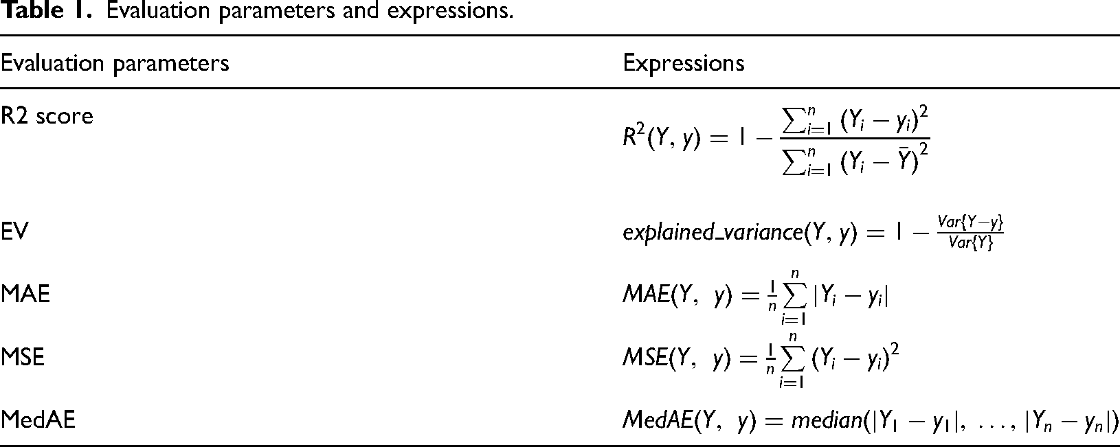
Some typical evaluation parameters such as R² score, explained variance score, mean absolute error, mean squared error and median absolute error are used to evaluate regression performance.

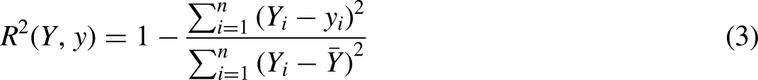
R² score

R² score refers to the determination coefficient, which is used to measure the effect of the model on the prediction of unknown samples, the best score is 1.0, and the value can be negative. Generally indicated by the symbol ‘R’. The expressions are as follows:

R^{2} (Y, y) = 1 - \frac{\sum_{i = 1}^{n} {(Y_{i} - y_{i})}^{2}}{\sum_{i = 1}^{n} {(Y_{i} - \bar{Y})}^{2}}

(3)

In the formula ‘y’ is the estimated target output, ‘Y’ is the corresponding (correct) target output, ‘y_i’ is the predicted value of the first sample, ‘Y_i’ is the corresponding true value, ‘n’ is the total number of samples, and ‘

\bar{Y}

’ is the average of the true value.

EV score

EV score (Explained variance score) is used to measure the ability of our model to interpret data set fluctuations, if the score is 1.0, means our model is perfect. The expressions are as follows:

explained_variance (Y, y) = 1 - \frac{V a r {Y - y}}{V a r {Y}}

(4)

In the formula ‘y’ is the estimated target output, ‘Y’ is the corresponding (correct) target output, ‘Var’ is the variance.

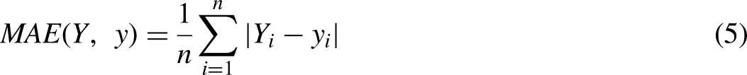
MAE

MAE (mean absolute error) is the absolute error average of all data points for a given dataset. The smaller the value, the better the prediction effect. The expressions are as follows:

M A E (Y, y) = \frac{1}{n} \sum_{i = 1}^{n} | Y_{i} - y_{i} |

(5)

MSE

MSE (mean squared error) is the average of the square of all data points in a given dataset and it is the most popular index. The smaller its value, the better the prediction effect. The expressions are as follows:

M S E (Y, y) = \frac{1}{n} \sum_{i = 1}^{n} (Y_{i} - y_{i})^{2}

(6)

Medae

MedAE (median absolute error) is the median error of all data points for a given dataset and it can eliminate the interference of outliers. The smaller the value, the better the prediction effect. The expressions are as follows:

M e d A E (Y, y) = median (| Y_{1} - y_{1} |, \dots, | Y_{n} - y_{n} |)

(7)

The closer the accuracy is to 100%, the closer the R² and the explained variance score is to 1, the smaller the mean absolute error, the mean squared error and mean absolute error are, the better the prediction effect is, that is, the more perfect the model is, otherwise the model is not good.

All evaluation parameters are summarized in Table 1.

Table 1.

Evaluation parameters and expressions.

Evaluation parameters	Expressions
R2 score	$R^{2} (Y, y) = 1 - \frac{\sum_{i = 1}^{n} {(Y_{i} - y_{i})}^{2}}{\sum_{i = 1}^{n} {(Y_{i} - \bar{Y})}^{2}}$
EV	$e x p l a i n e d_v a r i a n c e (Y, y) = 1 - \frac{V a r {Y - y}}{V a r {Y}}$
MAE	$M A E (Y, y) = \frac{1}{n} \sum_{i = 1}^{n} \| Y_{i} - y_{i} \|$
MSE	$M S E (Y, y) = \frac{1}{n} \sum_{i = 1}^{n} (Y_{i} - y_{i})^{2}$
MedAE	$M e d A E (Y, y) = m e d i a n (\| Y_{1} - y_{1} \|, \dots, \| Y_{n} - y_{n} \|)$

Case study

Data collection and processing

The data used in this study is the logging data in 31/2-N-23A Y1H well of Troll West field, which were reported by Hood (2003). The Troll West reservoir consists of the Upper Jurassic Sognefjord formation, a stacked series of sandstone units lying at a depth of approximately 1500 m below sea level. These sandstone units were formed by shoreline development on the northwestern edge of the Horda Platform during the Upper Jurassic. Clean medium to coarse-grained target sandstones alternate with finer, poorer quality non-target intervals. The shallow depth of burial has preserved good to excellent reservoir properties that are only locally reduced by calcite cementation. Calcite nodules and stringers up to several meters thick, derived from shell material within the sands, occur throughout the reservoir and can create difficulties for drilling.

The well logging data are presented in Figure 1. The data used are obtained from the logging curve of T1 well (31/2-N-23A Y1H well), which is digitally extracted by our team of homemade logging curve digital tools (http://www.petroleumcloud.cn/pages/21.html). The data presented in Figure 1 were recorded on Troll West in 2001 and 2002. These are depth-based log excerpts of drilling process data recorded at surface and downhole, along with formation data (Hood, 2003). The log excerpt shows data from the last 75 m of the reservoir section of T1 well.

Figure 1.

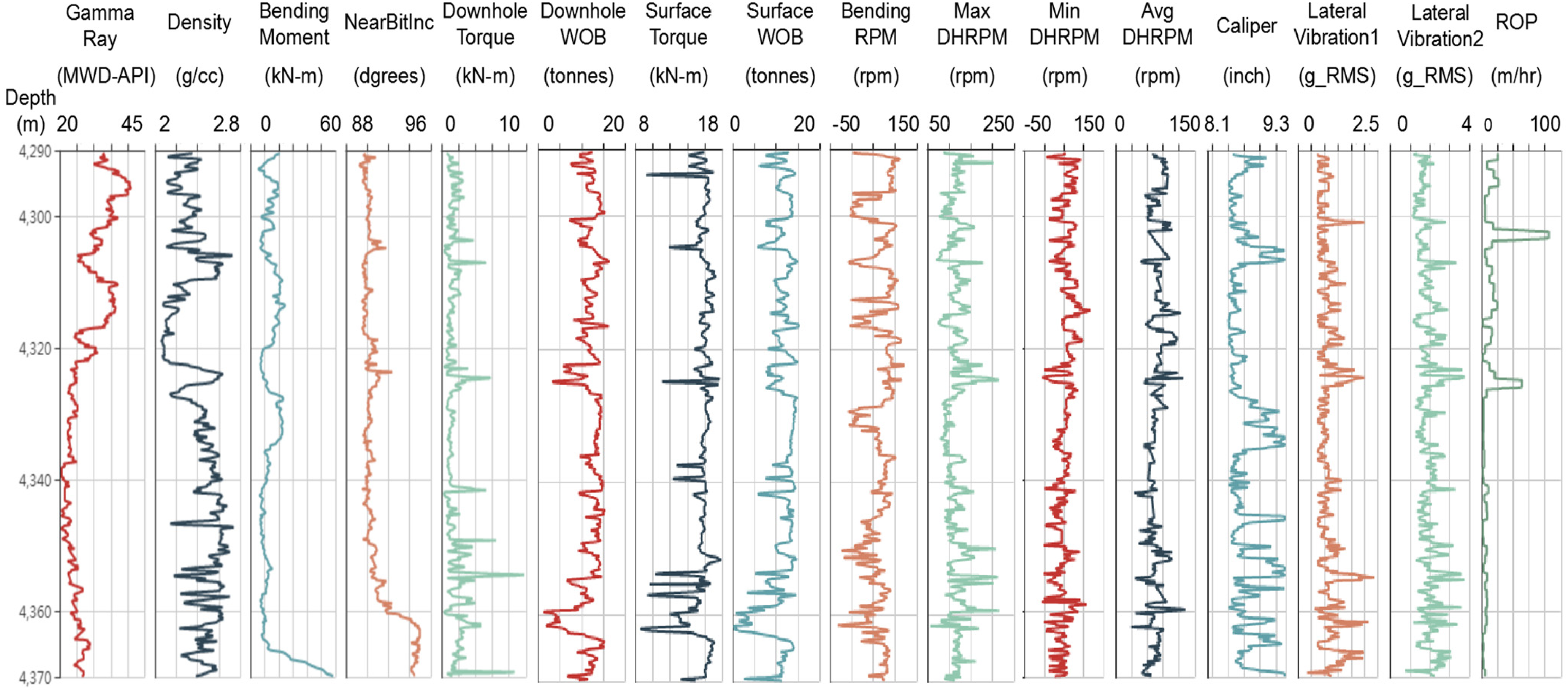
Logging data of well 31/2-N-23A Y1H.

In this paper, all the logging data are selected as the training set data, including Gamma Ray, Density, Bending Moment, Near Bit Inclination, Downhole Torque, Downhole WOB (Weight On Bit), Surface Torque, Surface WOB, Bending RPM (Revolutions Per minute), Max DH RPM, Min DH RPM, Avg DH RPM, Caliper, Lateral Vibration1, and Lateral Vibration2 with the depths ranging from 4290 m to 4370 m.

Data pre-processing

791 readings from T1 well (well 31/2-N-23A Y1H) are collected to perform the evaluation. Each data point is preprocessed with 15 features mentioned above. First, the discrete data obtained from the different logging curves are interpolated and the logging data are aligned by well depth. These collected logging features for each data point are arranged into a matrix to ensure that all the logging features in the rows are aligned to the same well depth, where the number of behavioral instances, fifteen columns contain the described features, and one column contains the true ROP. A model comparison scheme is carried out to find a suitable model for the target well logging data.

The dataset is divided into a training set and a test set according to a certain ratio for different purposes. In order to consider all lithologic strata, four points out of every five points in the data series were selected to train the learning model, and the rest of the data were used as test sets. The data points accounting for 80% of the entire data set are selected as the training set, and every point in the training set will be used to train the learning model. The rest of the data is used as the test set. Since the proportion of training data in the entire dataset and the sampling method affect the test results, the sampling method is the same for different model comparison schemes.

Model performance comparison

This section applied machine learning regression algorithms to predict ROP. By using scikit-learn, a machine learning module in Python that integrates a rich set of regression algorithms, it provides simple, easy-to-use, and efficient data analysis tools to evaluate the performance of the regressors. Four typical regression algorithms are used to predict ROP: SVR, linear regression, GBR, and regression tree. To meet the needs of drilling operations, the prediction results of different methods are compared to find a suitable method with high accuracy and low computation time. Evaluation parameters such as R2 score, explained variance score, mean absolute error, mean squared error and median absolute error are used to evaluate the prediction results. In general, the closer the R2, explained variance is to one, the smaller the mean absolute error, mean squared error and median absolute error, and the more accurate the prediction.

Figure 2 shows the prediction results when SVR, linear regression, GBR algorithm and regression tree are used to predict the ROP for the T1 well. The solid blue line is the predicted ROP and the dashed green line is the true ROP. From left to right are the prediction results of GBR algorithm, regression tree, SVR and linear regression methods, with decreasing accuracy from left to right.

Figure 2.

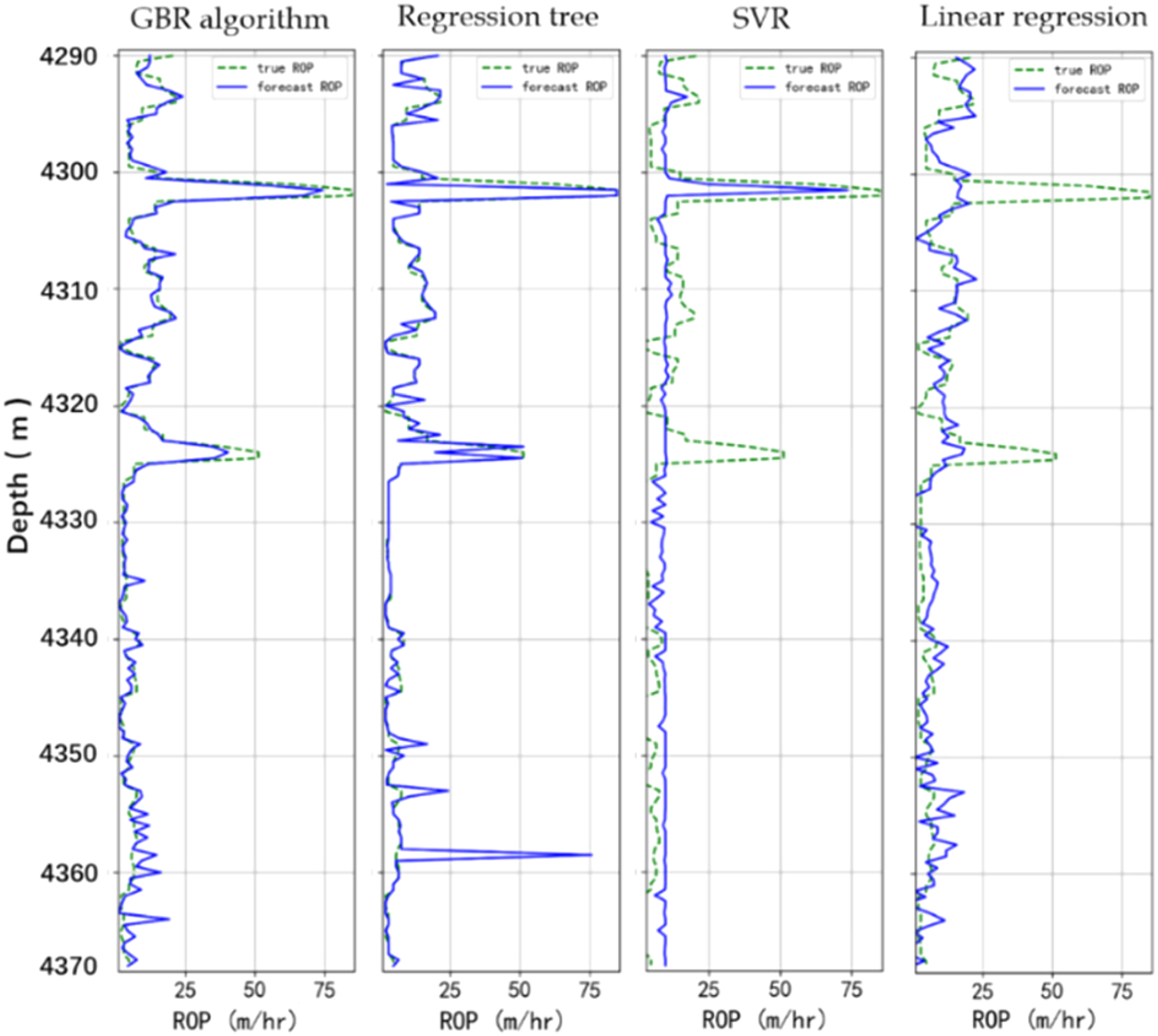
Prediction results of ROP for well 31/2-N-23A Y1H.

It can be seen from the comparison curve that the coincidence degree between the predicted ROP curve and the real ROP curve is the highest when GBR algorithm is used, but the coincidence of SVR method is very few. It can be seen from Figure 2 that the overall trend of the ROP decreases with the deepening of depth, and is basically less than 25 m/h, and the ROP is basically kept below 10 m/h when the depth is greater than 4320 m. When the depth is about 4301–4303 m, the ROP suddenly increases, from 15 m/h to about 85 m/h. At a depth of about 4324–4326 m, there is also a mutation in the ROP, which increases from 20 to 50 m/h. Of the above four methods, GBR algorithm and Regression tree can fit the mutation, the other two do not have this ability, but compared with regression tree, GBR algorithm prediction is more accurate. As for the whole ROP curve, the predicted ROP curve using GBR algorithm method has the highest coincidence degree with the real curve. This is because the GBR algorithm is a technique for learning from its mistakes. Its main idea is that each time the loss function of the model is set up, it decreases in the direction of its gradient.

Precision comparison is shown in Table 2.

Table 2.

Model performance comparison for ROP prediction of well 31/2-N-23A Y1H.

Model	GBR algorithm	Regression tree	SVR	Linear regression
R²	0.90	0.52	0.35	0.21
EV	0.90	0.52	0.35	0.21
MAE	2.37	2.38	5.86	5.48
MSE	15.40	70.99	96.48	116.17
MedAE	1.28	0.00	4.42	3.69
T(s)	0.9845	0.2791	0.0675	0.0133

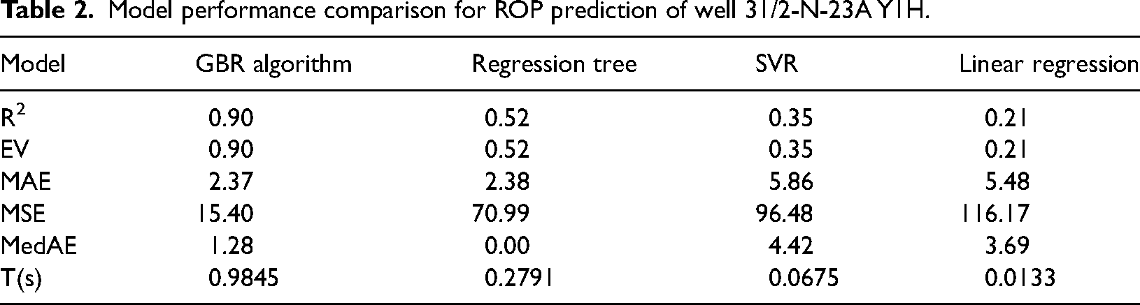
In Table 2, R² refers to the deterministic correlation coefficient, EV is Explained variance score. The closer the value of R² and EV is to one, the better the prediction is. MAE is mean absolute error, MSE is mean squared error and MedAE refers to median absolute error. The smaller the value of these evaluation parameters, the better the prediction. T refers to the time spent on this model calculation. The shorter the time spent in the calculation, the more efficient the model is.

It can be seen from Table 2 that the GBR algorithm has the best effect in predicting ROP. The R² and the EV are the highest in the four methods, reaching 0.90. MAE and MSE are also the lowest of the four methods, where MAE is only 2.37, MSE is 15.40. And among these four methods, the effect of Linear regression in predicting ROP is the worst., which the R² is 0.21 and the EV is the same 0.21. MAE and MSE reach 5.36 and 119.55, respectively, and the MedAE is at the middle level.

All of these methods are fast, with the exception of GBR, which has a prediction time of nearly 1 s, the other three methods have a prediction time of under 0.3 s. The fastest prediction is SVR, which took less than 0.01 s.

Model parameter analysis

Each algorithm model contains specific parameters, which can be adjusted to improve the accuracy of prediction. Taking GBR algorithm as an example, the parameter adjustment process of GBR algorithm is shown in the figure below. This method is based on the logging data of well T1, and six times of cross validation are adopted.

The performance of the GBR algorithm is mainly affected by the learning rate ν. For the GBR algorithm, learning rate ν, estimator number n_e and subsample S is the key parameter to investigate. ν is the learning rate, which represents the contribution of each tree. n_e is the estimator number, represents the number of boosting stages to perform. S is subsample, the fraction of samples to be used for fitting the individual base learners.

The sweeping range and optimum value of ν, n_e and S for GBR are shown in the Table 3. Figure 3 (a) - (c) show the ROP prediction results after parameter adjustment. The green dotted line indicates the true ROP, and the blue solid line indicates the predicted ROP:

Figure 3.

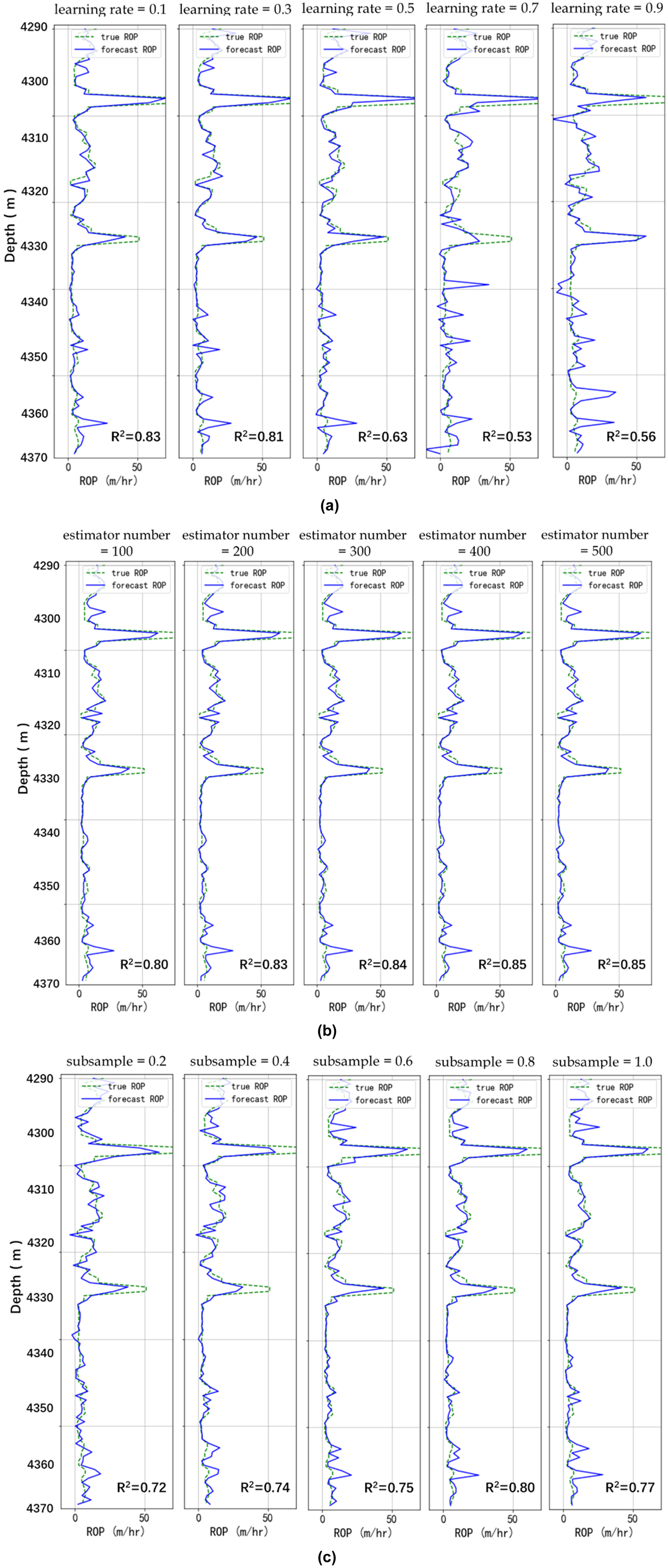
Parameter tuning result for GBR. (a) the learning rate. (b) the estimator number. (c) the subsample.

Table 3.

Parameter tuning for GBR model training.

Parameter	Function	Sweeping range	Optimal value
Learning rate, ν	The contribution of each tree	0.1–1	0.1
Estimator number, n_e	The number of boosting stages to perform.	50–450	400
Subsample, S	The fraction of samples to be used for fitting the individual base learners	0–1	0.8

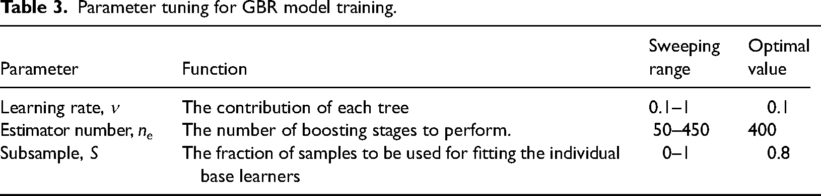
The comparison of the prediction results (Figure 3) shows that GBR models with smaller learning rate and larger estimator number and subsample tend to obtain higher prediction accuracy. The prediction accuracy is more sensitive with ν and S. The prediction results show that when the Learning rate is 0.1, the prediction effect is the best, and the R² is 0.83. And the best prediction of ROP is achieved when the estimator number is 400. That is, when the ν = 0.1, n_e = 400 and S = 0.8, the validation accuracy is highest and the standard deviation is smallest. The GBR model works best when the ν is 0.1, n_e is 400 and S is 0.8.

Results and discussion

Effect of the amount of training data on prediction accuracy

Varying the percentage of the training set and predicting the ROP showed a big difference in the prediction results. In the figures, the horizontal coordinate is the proportion of the training set and the vertical coordinate is each evaluation parameter, showing the variation of the prediction effect of different methods with different training set percentages:

From the algorithm mentioned above, the closer the R² is to 1, the better the prediction performance. As shown in Figure 4, the GBR algorithm predicts best when the training set accounts for 75% of the total set, and the regression tree. The linear regression and SVR methods have the best prediction performance when the training set is 50% of the total set. In general, the GBR algorithm has the best prediction performance.

Figure 4.

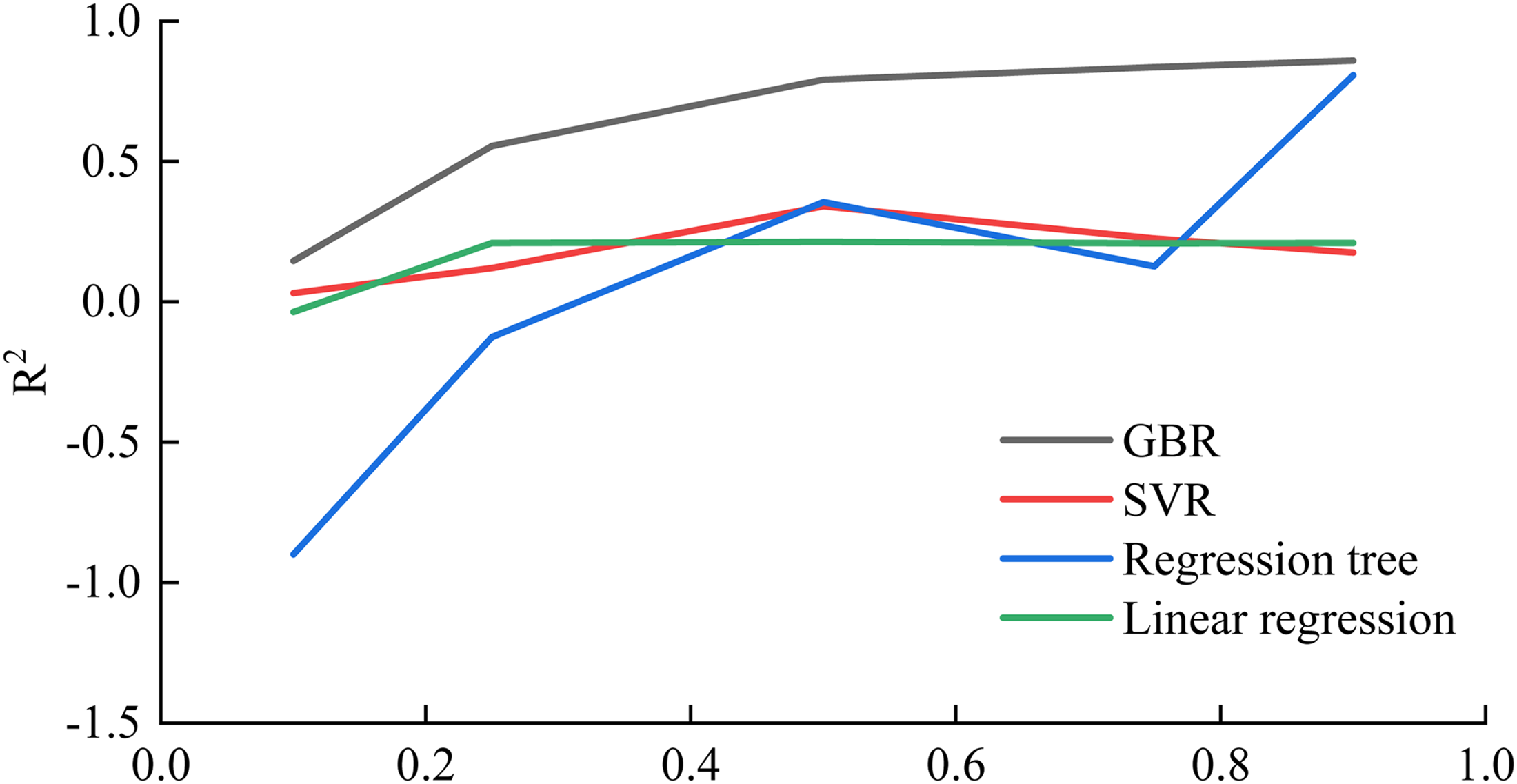
R2 at different training set percentages.

As with R², the closer the EV is to 1 the better the prediction is. As shown in Figure 5, the results are almost the same as the R² results. Prediction accuracy increases with increasing training sets. The percentage of the training set that resulted in the best predictive performance varied by method. And the GBR algorithm always has the best prediction performance.

Figure 5.

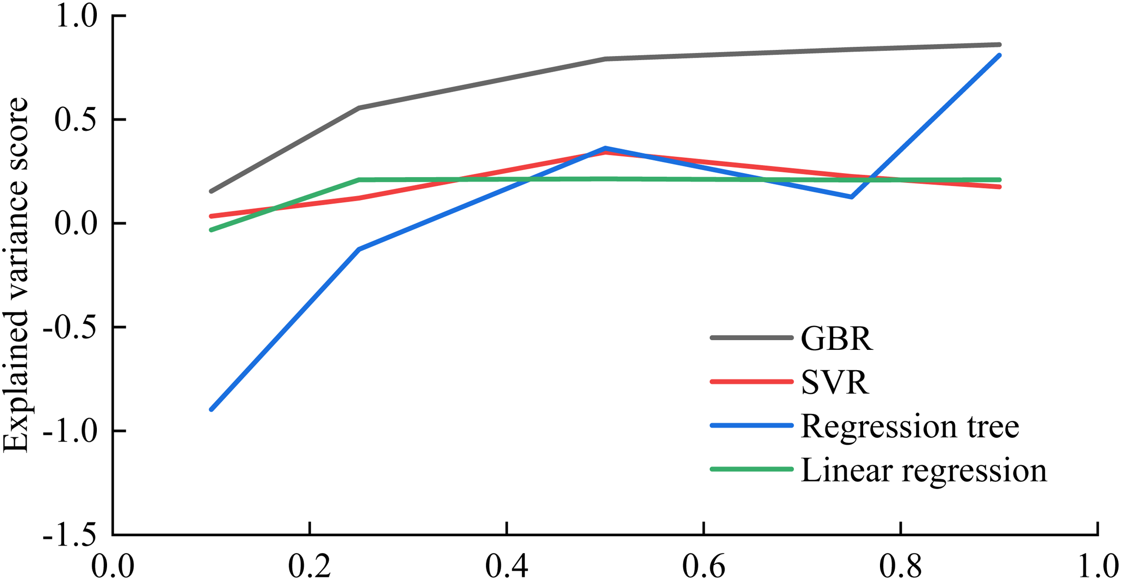
Ev at different training set percentages.

As shown in Figure 6, the smaller the MAE, the better the prediction. In general, the MAE slowly decreases as the training set increases. All methods except regression tree predicted best at 75% of the training set. The GBR algorithm and regression tree have the best prediction performance.

Figure 6.

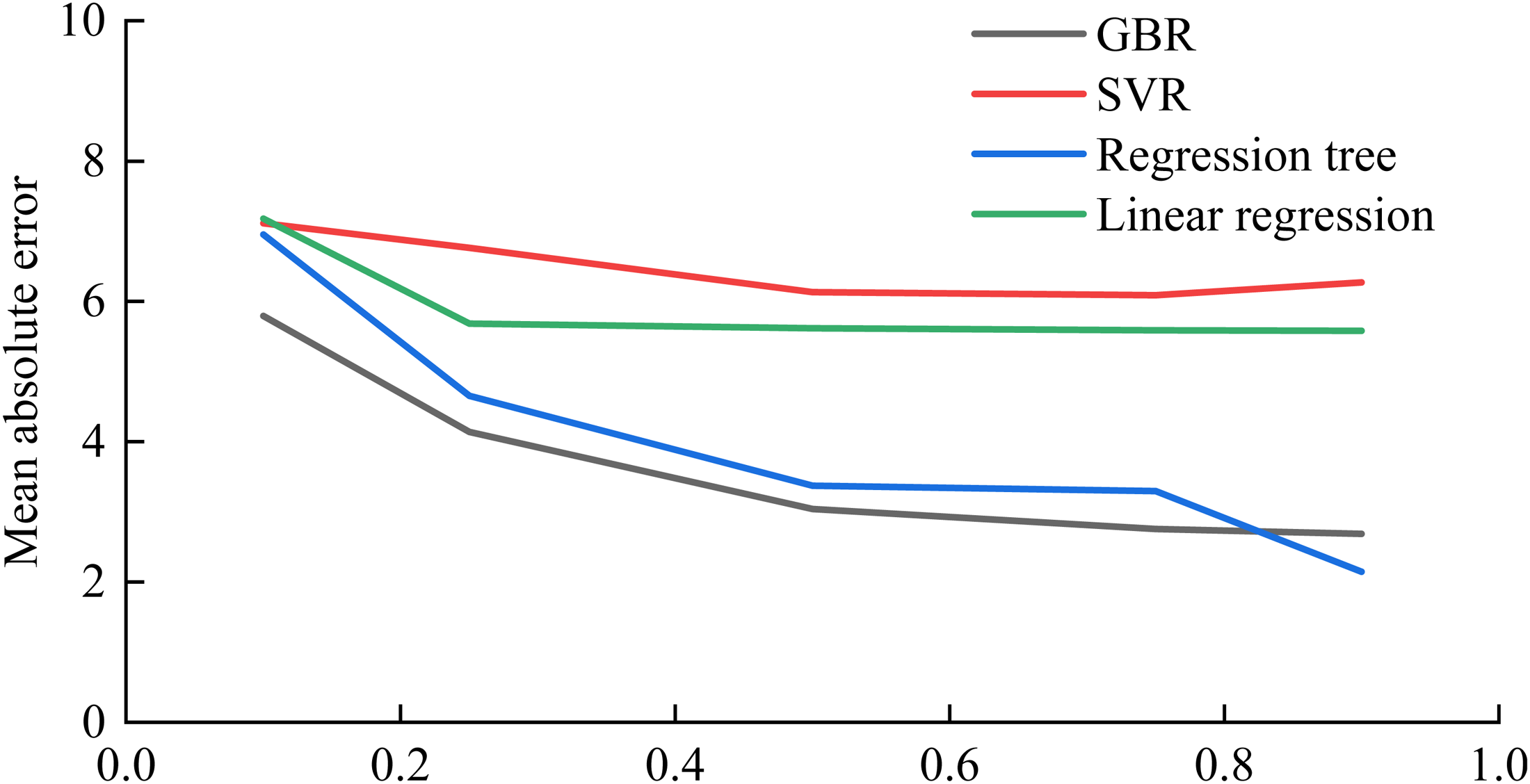
MAE at different training set percentages.

The smaller the MedAE, the better the prediction. In general, the more training sets, the lower the MedAE, the better the prediction. As can be seen from Figure 7, the MedAE does not change much. The Regression tree has the best prediction performance.

Figure 7.

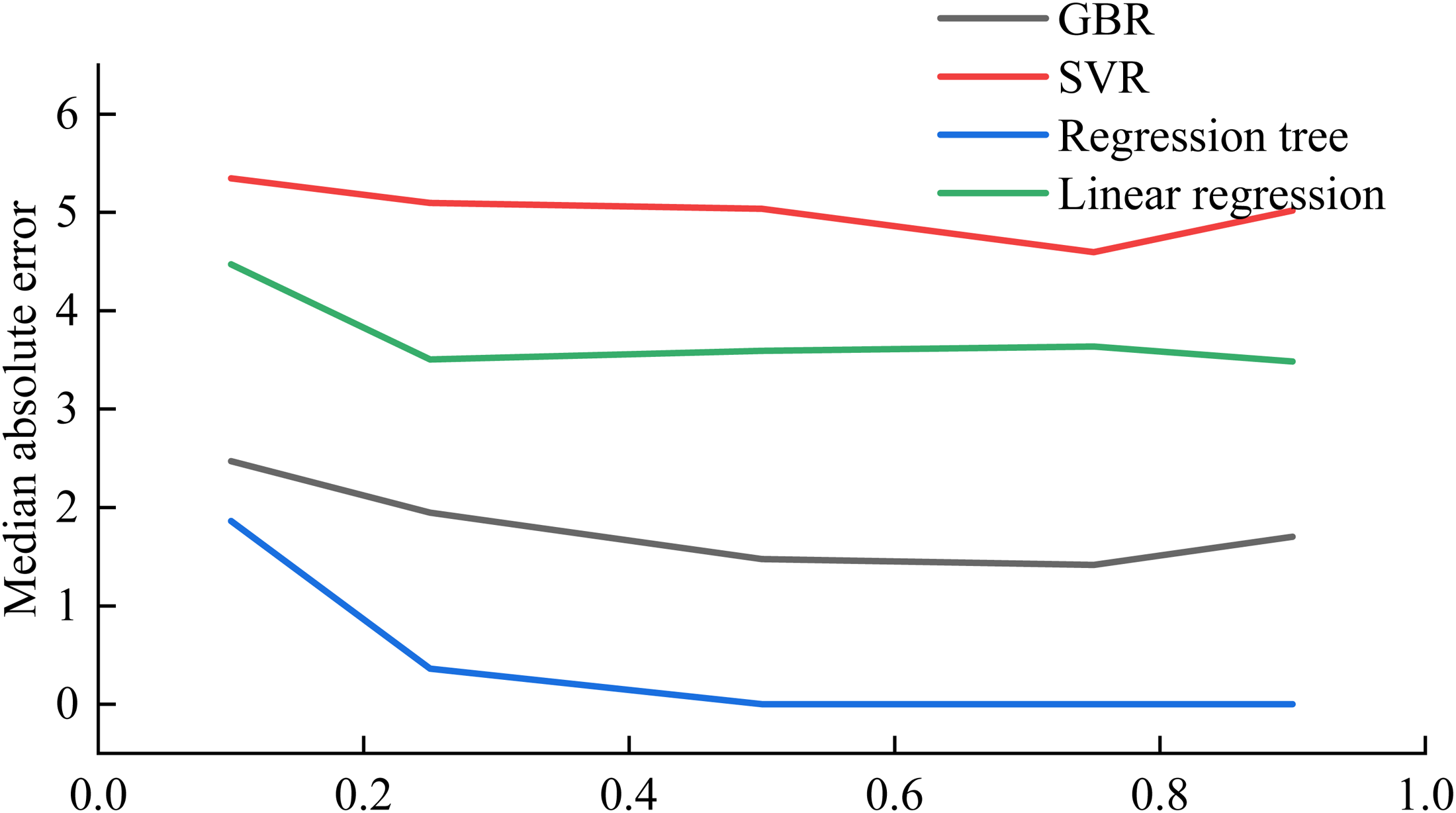
MedAE at different training set percentages.

The smaller the MSE, the better the prediction. As can be seen in Figure 8, the MSE of all other methods decreases as the training set increases. The GBR algorithm always has the best prediction performance.

Figure 8.

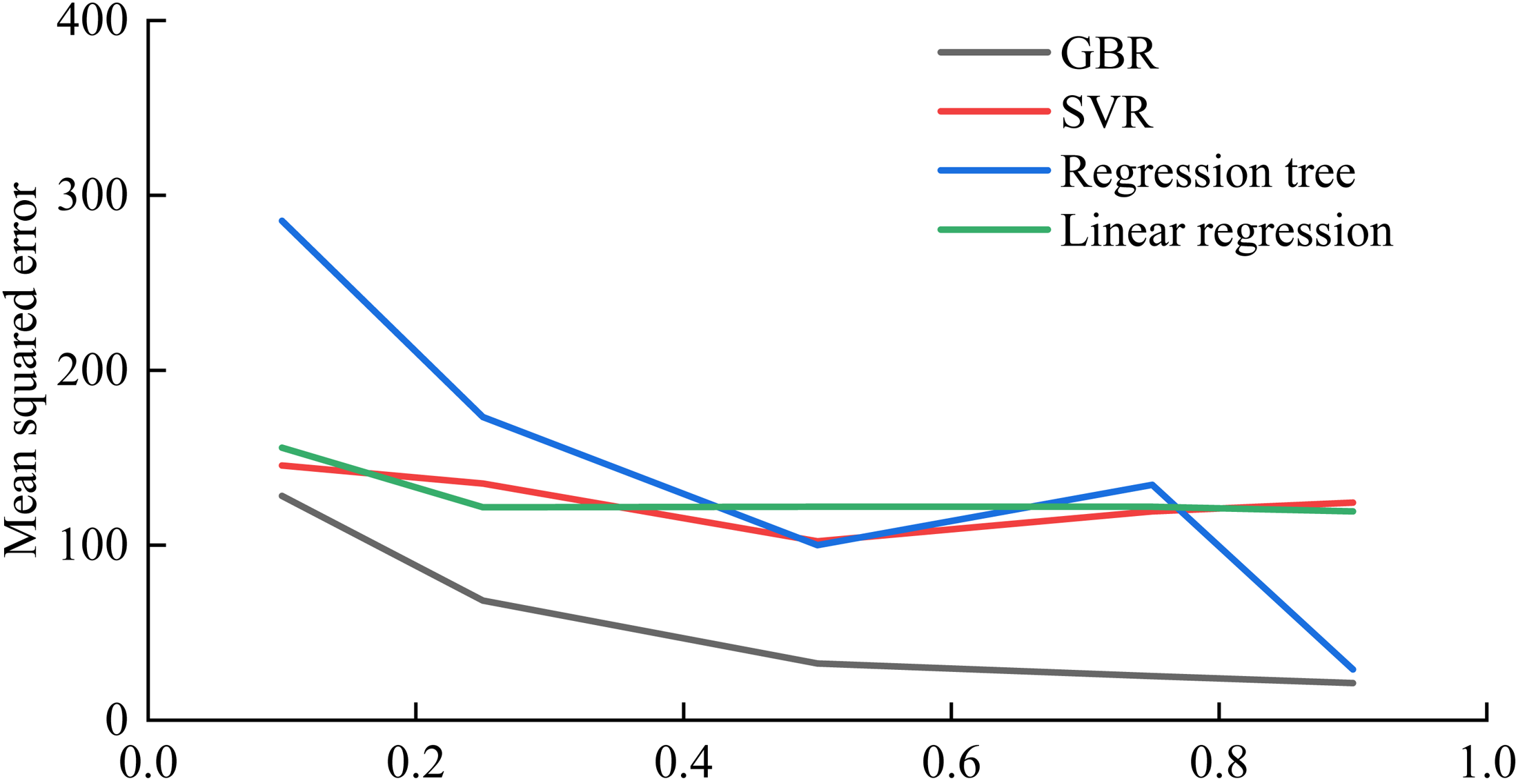
MSE at different training set percentages.

In general, the higher the percentage of training data, the better the ROP prediction. GBR algorithm is the best method to predict ROP. For the GBR algorithm, when using 75% of the data as training data, the prediction is the best.

Parameter combination analysis

The data has 15 parameters, including Gamma Ray, Density, Bending Moment, Near Bit Inclination, Downhole Torque, Downhole WOB, Surface Torque, Surface WOB, Bending RPM, Max DH RPM, Min DH RPM, Avg DH RPM, Caliper, Lateral Vibration1, and Lateral Vibration2. The parameters are represented by codes, as shown in Table 4.

Table 4.

Parameters representation.

Parameters	code
Gamma Ray	G
Density	D
Bending Moment	BM
Near Bit Inclination	NBI
Downhole Torque	DT
Downhole WOB	DW
Surface Torque	ST
Surface WOB	SW
Bending RPM	BR
Max DH RPM	MaxR
Min DH RPM	MinR
Avg DH RPM	AvgR
Caliper	C
Lateral Vibration1	LV1
Lateral Vibration2	LV2

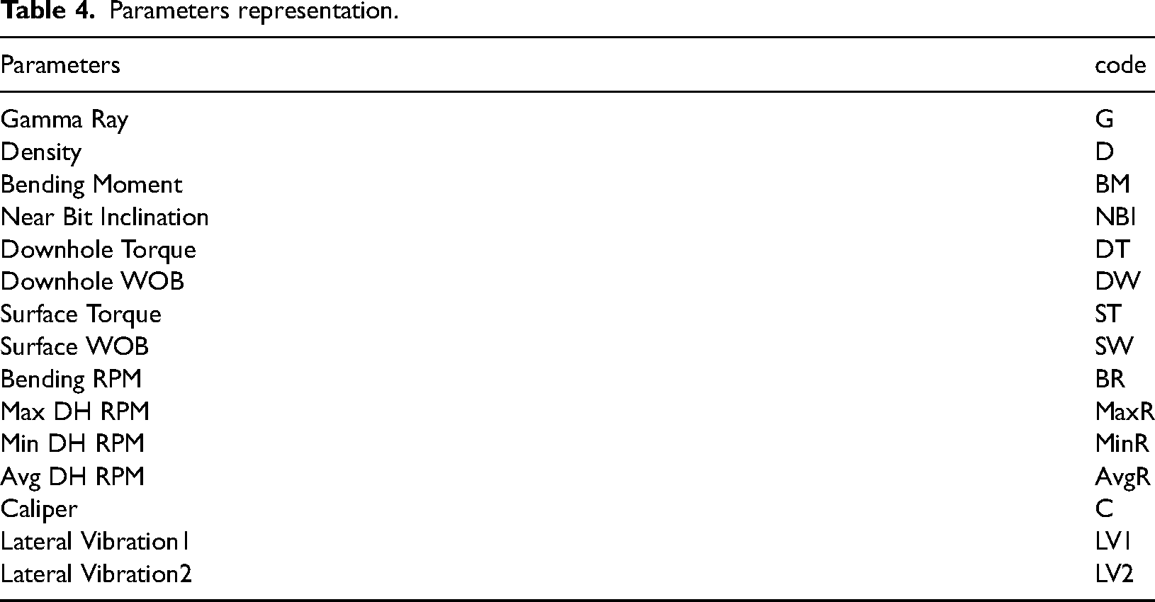
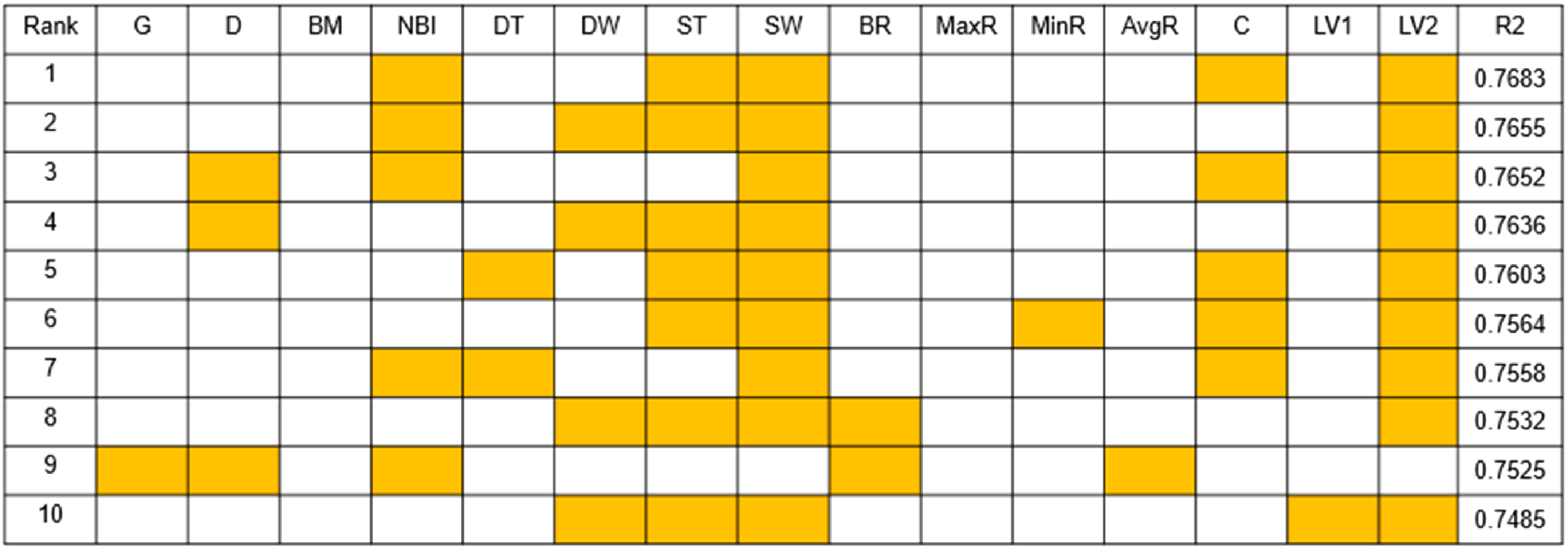
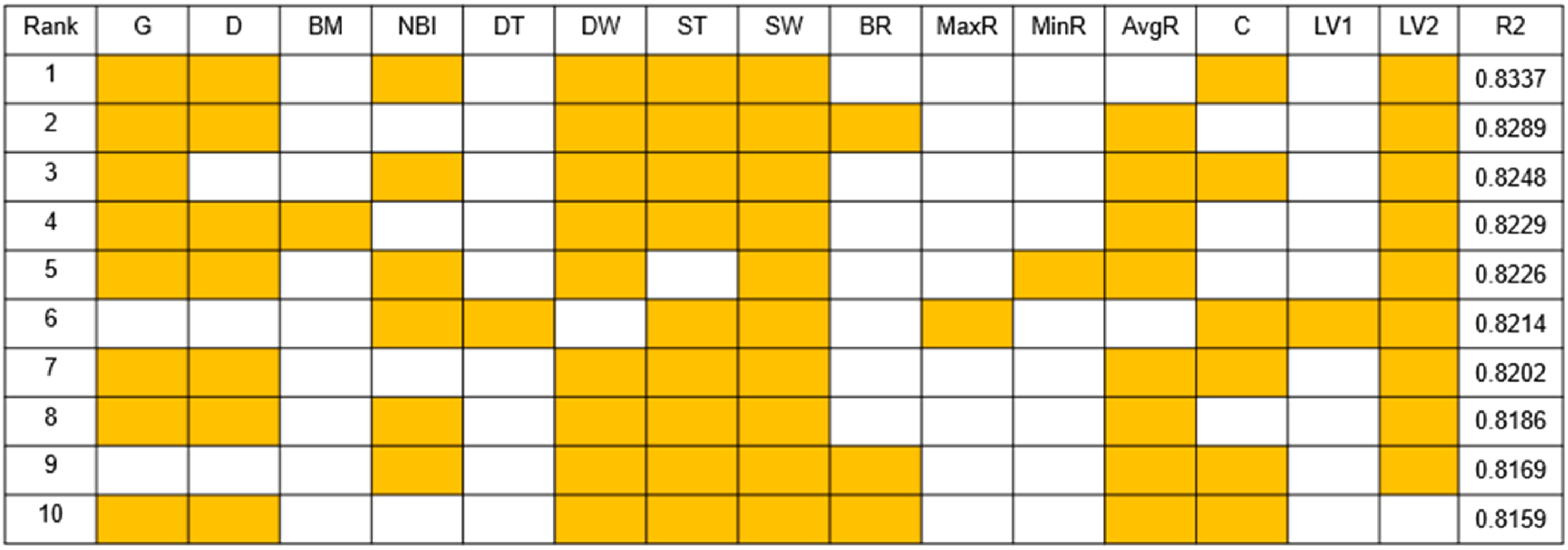
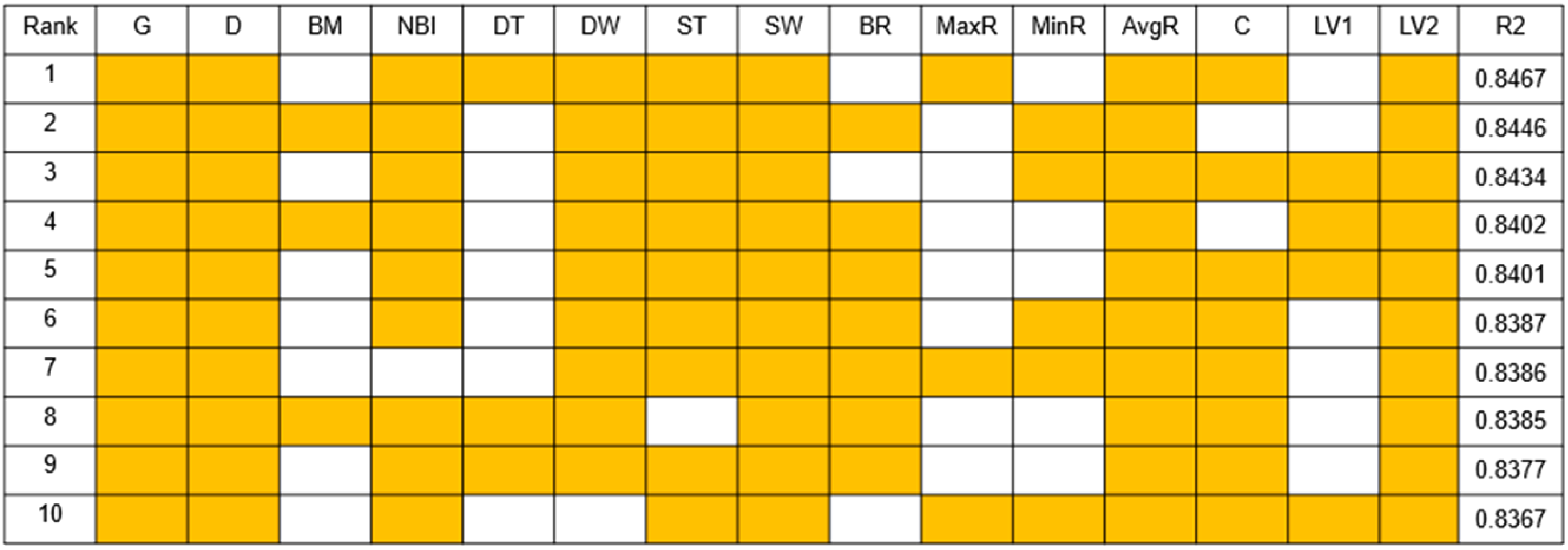
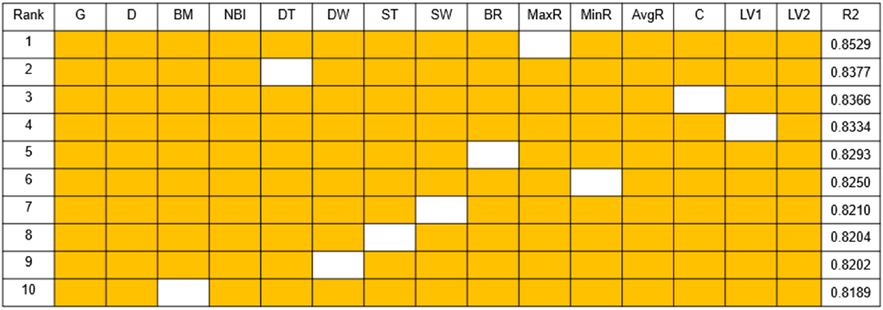
The method of dimension reduction is used to predict the ROP of different parameter combinations. Random combinations of 2, 5, 8 and 11 parameters are selected from the 15 indicators respectively, and the top 10 combinations are displayed from highest to lowest according to the magnitude of the R² score. Only using the GBR algorithm and using 75% of the data as a training set, the parameter combinations and prediction results are shown below.

As can be seen from Figure 9 through Figure 13, the more parameters, the better the prediction. And parameters such as Bending Moment, Downhole Torque, Bending RPM, Max DH RPM, Caliper and Lateral Vibration1 are not good for ROP prediction, while parameters such as Gamma Ray, Density, Near Bit Inclination, Downhole WOB, Surface Torque, Surface WOB and Lateral Vibration2 are favorable to the prediction of ROP.

Figure 9.

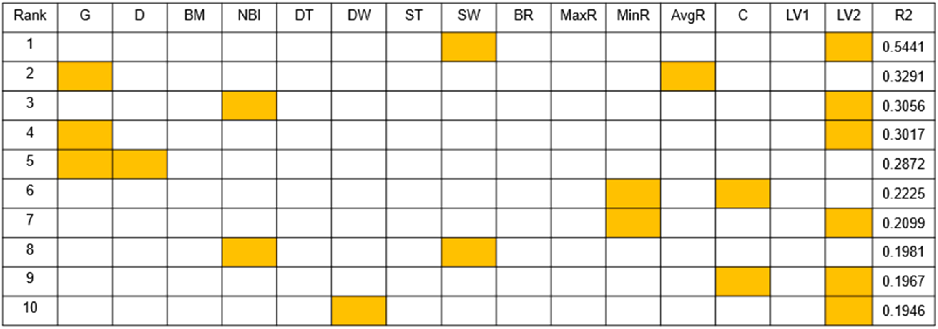
Two Parameters combination results.

Figure 10.

Five Parameters combination results.

Figure 11.

Eight Parameters combination results.

Figure 12.

Eleven Parameters combination results.

Figure 13.

Fourteen Parameters combination results.

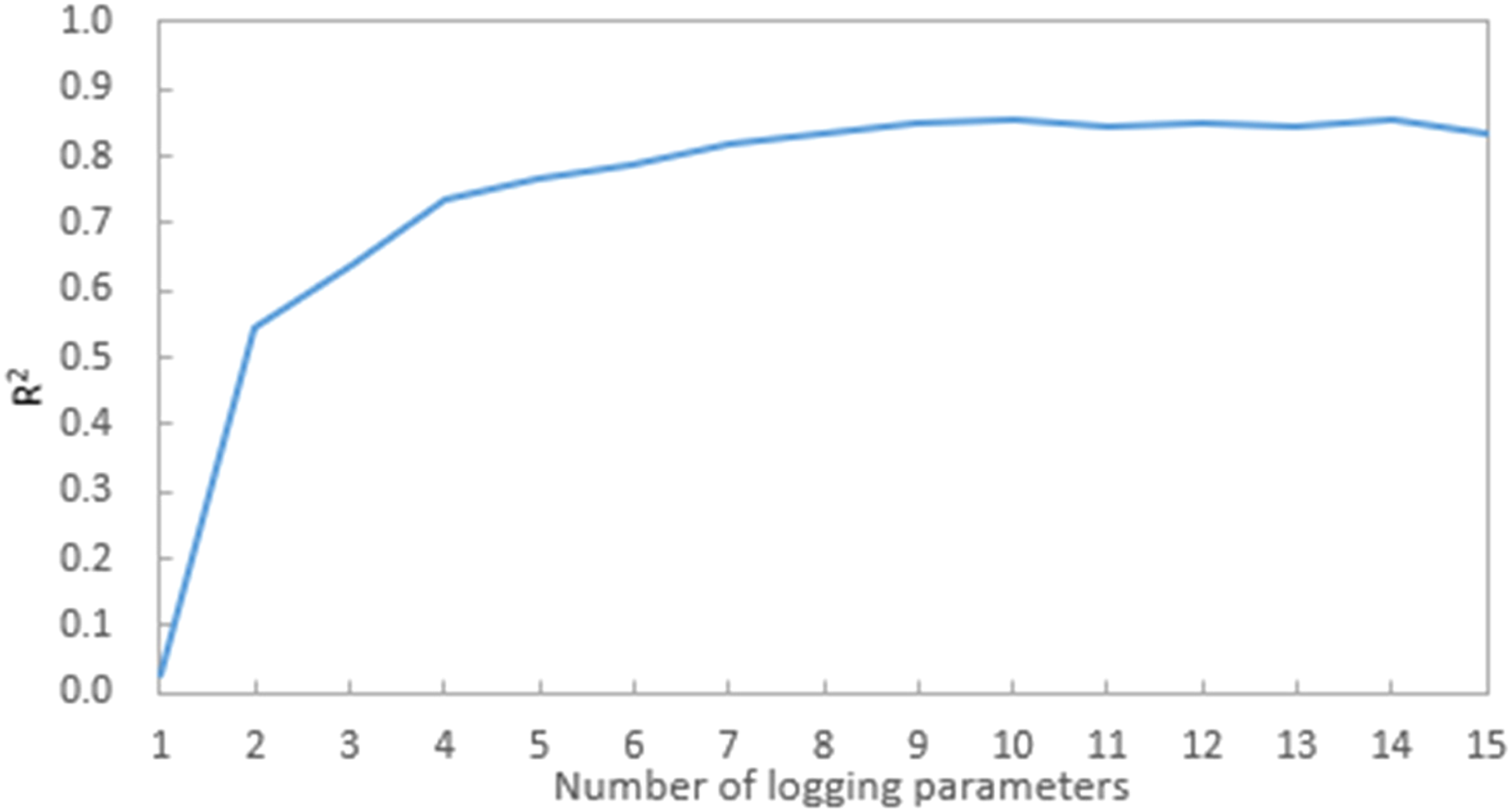
Figure 14 and Figure 15 shows that the accuracy of predicting ROP when using only one parameter is almost 0, starting from two parameters, the accuracy of predicting the ROP gradually increased, when using 7 parameters, R² reached 0.8, and then increase the parameters R² also remain at 0.8 or so. When 10 parameters are used, the predicted ROP R² reaches a maximum of 0.8542, at which point the parameter combination is Gamma Ray, Density, Near Bit Inc, Downhole WOB, Surface Torque, Surface WOB, Max DH RPM, Min DH RPM, Avg DH RPM and Lateral Vibration2.

Figure 14.

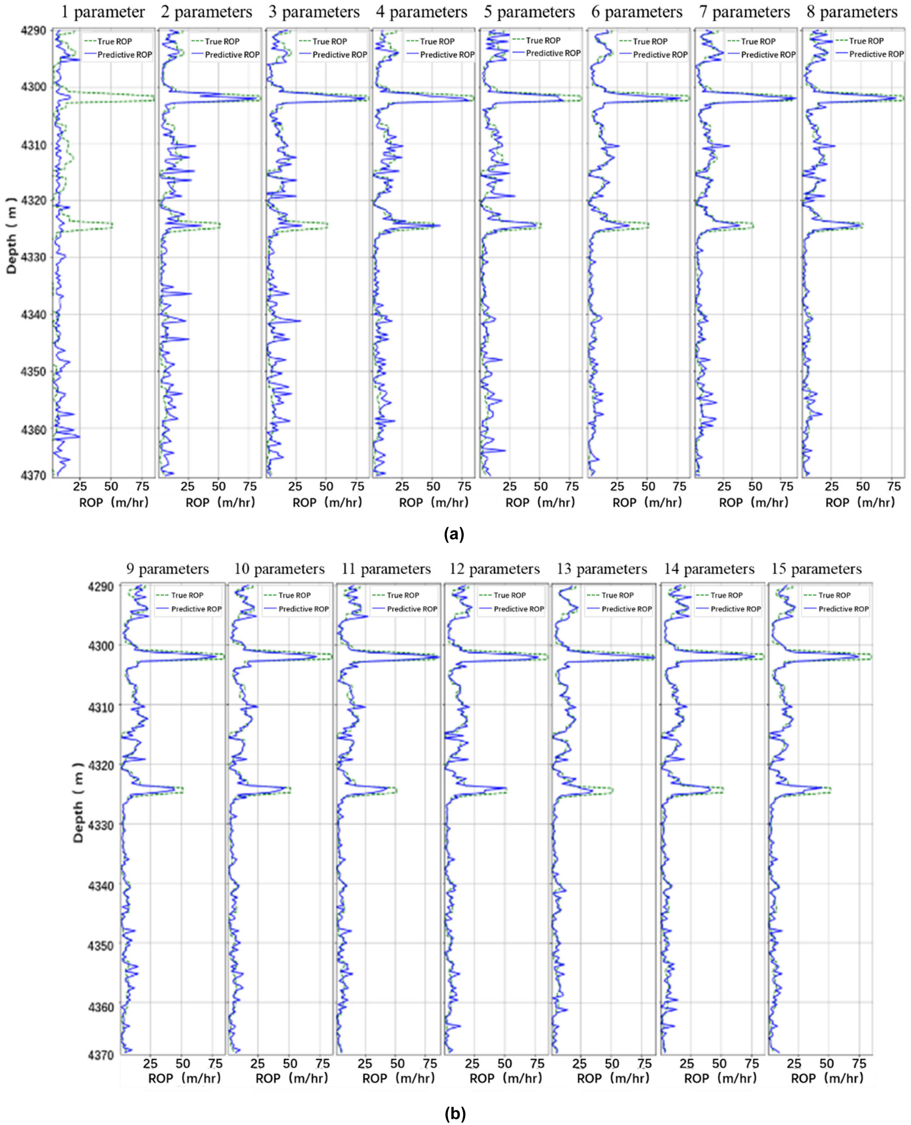
Prediction results of dimension reduction. (a) 1∼8 parameters. (b) 9∼15 parameters.

Figure 15.

Dimension reduction calculation results.

Neighboring well prediction

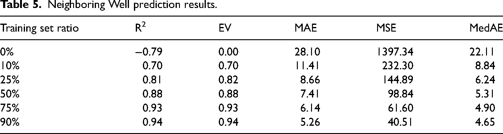
T2 Well (well 31/2-N-21 Y1H) is a neighboring well to T1 well. The same logging data as T1 well is collected and the model from T1 well is used to predict the drilling rate for T2 well. GBR algorithm is used for neighboring well prediction. The results are as follows:

All of the T1 well logging data were used as training data, and data of T2 well were gradually added as training data to training model. Prediction results vary with the added training sets ratio of T2 well.

It can be seen from Table 5 that when only use the data of T1 well to predict the ROP of T2 well, the prediction is poor and does not allow for neighboring well prediction. When add at least 25% data of T2 well as training data, the R² reached above 0.8 and predicted the ROP of T2 well better.

Table 5.

Neighboring Well prediction results.

Training set ratio	R²	EV	MAE	MSE	MedAE
0%	−0.79	0.00	28.10	1397.34	22.11
10%	0.70	0.70	11.41	232.30	8.84
25%	0.81	0.82	8.66	144.89	6.24
50%	0.88	0.88	7.41	98.84	5.31
75%	0.93	0.93	6.14	61.60	4.90
90%	0.94	0.94	5.26	40.51	4.65

In contrast to previous studies in the introduction which have focused on the training of a single model or algorithm, this paper focuses its attention on four regression algorithms, comparing the advantages and disadvantages of the four algorithms horizontally to facilitate the selection of practical applications in the field according to the actual requirements.

Conclusion

Four typical regression algorithms based on machine learning such as SVR, Linear regression, GBR algorithm and Regression tree method are used for ROP prediction. These methods can allow more parameters to be considered while drilling and the prediction accuracy is high. Evaluation parameters such as R², EV (Explained variance score), MAE (mean absolute error), MSE (mean squared error), and MedAE (median absolute error) were used to evaluate the prediction results. Based on the logging data from T1 well, six-fold cross-validation was used to adjust certain parameters used in the four regression models to a certain extent to help the regression algorithm perform better. The effect of data set occupancy on regression prediction is analyzed, the regression accuracy of different parameter combinations is compared, and the parameter combination that makes the best prediction is derived, and finally the drilling rate of neighboring well T2 is predicted, the details are as follows:

Among the four methods for ROP prediction, GBR algorithm has the highest prediction score, followed by regression tree, SVR and linear regression. Therefore, GBR algorithm can be used in field application to predict the ROP.

Although the GBR method has the best prediction result, its computation time is the longest among the four methods. In general, the better the prediction effect, the longer the use time. When the calculation time is not considered, the GBR algorithm can be preferred.

The accuracy of all four methods for ROP prediction was positively correlated with the proportion of the training data set. By using 75% of the dataset for training, better predictions can be achieved. Therefore, in practical application, it is necessary to find the best percentage of training set according to the situation.

The accuracy of prediction gradually improves as the number of logging features increases. This improving trend becomes gradually slower when the number of logging features exceeds 4, and the accuracy can reach 80% for most combinations of more than 7 logging parameters. Therefore, in field application, as many logging features as possible should be used to improve the prediction accuracy.

When neighboring wells are predicted, the higher the percentage of neighboring well data added to the training set the best training effect, and when 25% of neighboring well data is added as the training set, the accuracy can reach more than 80%.

Through the prediction process, it showed that using GBR algorithm has the highest accuracy among all the used algorithms. For the used data, the best combination of parameters for GBR algorithm are Gamma Ray, Density, Near Bit Inc, Downhole WOB, Surface Torque, Surface WOB, Max DH RPM, Min DH RPM, Avg DH RPM and Lateral Vibration2. This method can predict the ROP in real-time, provide the basis for safe and efficient drilling, and provide technical support for the development of intelligent drilling. Therefore, without taking into account the calculation time, the relevant group decision-makers can use the GBR algorithm, combined with the relevant parameters mentioned above, to make forecasts, improve the accuracy of forecasts and carry out optimal resource allocation.

The regression algorithm selected in this study is relatively general, so it lacks some innovation in algorithm selection. Future research will focus on introducing more machine learning algorithms for drilling speed to investigate the performance of different methods in predicting ROP on logging data.

Footnotes

Declaration of conflicting interests

The author(s) declared no potential conflicts of interest with respect to the research, authorship, and/or publication of this article.

Acknowledgement

The present research is supported by PetroChina Innovation Foundation (Grant No. 2020D-5007-0308), the Strategic Cooperation Technology Projects of CNPC and CUPB (Grant No. ZLZX2020-03), National Key Research and Development Project (Grant No. 2019YFA0708300), the Strategic Priority Research Program of the Chinese Academy of Sciences (Grant No. XDA14040402), the Key core technology research project of CNPC(Grant No. 2020B-4019) and Projects of CNPC (No.2021DQ0503).

ORCID iD

Ting Sun

Appendix

GBR model training steps are as follows:

① Input training set $T = {(x_{1}, y_{1}), (x_{2}, y_{2}) \dots, (x_{N}, y_{N})}, x_{i} \in ℵ \subseteq R^{n}, y \in Y \subseteq R^{n}$ and loss function $L (y, f (x))$ . Calculate: (8)

f_{0} (x) = \arg min_{c} \sum_{i = 1}^{N} L (y, c)

② Training rounds m = 1,2,…,M

Calculate the residual of model (9)

r_{m i} = - {[\frac{\partial L (y_{i}, f (x_{i}))}{\partial f (x_{i})}]}_{f (x) = f_{m - 1} (x)}, i = 1, 2, \dots, N

The value of the negative gradient of the loss function on the current model

F_{m - 1} (x)

is used to approximately replace the residual.

Fit r_mj and generate CART tree

Calculate (10)

c_{mj} = \arg min_{c} \sum_{x_{i} \in R_{m j}} L (y_{i}, f_{m - 1} (x_{i}) + c), j = 1, 2, \dots, J

In which R_mj is the leaf node area, J is the number of leaf nodes of the model.

Update (11)

f_{m} (x) = f_{m - 1} (x) + \sum_{j = 1}^{J} c_{m j} I (x_{i} \in R_{m j})

③ Input GBR model (12)

\hat{f} (x) = f_{M} (x) = \sum_{i = 1}^{N} \sum_{j = 1}^{J} c_{m j} I (x \in R_{m j})

The formula describing the process of regression tree is as follows: (13)

\underset{j s}{m i n} [\underset{c_{1}}{m i n} L o s s (y_{i}, c_{1}) + \underset{c_{2}}{m i n} L o s s (y_{i}, c_{2})]

to find the optimal j and s is obtained by comparing the different divided errors. The error of the division of an input space is measured by the least squares of the real value and the predicted value of the divided area, i.e.,: (14)

\sum_{x_{i} \in R_{m}} (y_{i} - f (x_{i}))^{2}

Where f (x_i) is the predicted value of each partition unit, which is the mean value of each sample point in the unit. Suppose the input space is divided into M units: R₁, R₂,. R_m, then the output value for each region is:

f (x_{i}) = c_{m} = a v e (y_{i} | x_{i} \in R_{m})

.That is, the average of all points in the area.

Then the solving of j and s can be carried out using the following equation: (15)

min_{j, s} [{min}_{c_{1}} \sum_{x_{i} \in R_{1} (j, s)} {(y_{i} - c_{1})}^{2} + {min}_{c_{2}} \sum_{x_{i} \in R_{2} (j, s)} {(y_{i} - c_{2})}^{2}]

of which,

R_{1} (j, s) = {x | x^{j} \leq s}

and

R_{2} (j, s) = {x | x^{j} > s}

are the two areas that have been divided.

References

Al-AbdulJabbar

Mahmoud

Elkatatny

(2021) Artificial neural network model for real-time prediction of the rate of penetration while horizontally drilling natural gas-bearing sandstone formations. Arab J Geosci 14: 17.

Al-Betairi

Moussa

Al-Otaibi

(1988) Multiple regression approach to optimize drilling operations in the Arabian gulf area. SPE Drill Eng 3(01): 83–88.

Alum

Egbon

(2011) Semi-analytical models on the effect of drilling fluid properties on rate of penetration (ROP). In: Nigeria annual international conference and exhibition. Society of Petroleum Engineers. https://doi.org/10.2118/150806-MS

Bhattacharyya

Vyas

(2022b) Application of machine learning in predicting oil rate decline for Bakken shale oil wells. Scientific Reports 12: 16154.

Bhattacharyya

Vyas

(2022c) Machine learning-based rate decline prediction in unconventional reservoirs. Upstream Oil and Gas Technology 8: 100064, ISSN 2666-2604.

Bhattacharyya

Vyas

(2022a) A novel methodology for fast reservoir simulation of single-phase gas reservoirs using machine learning. Heliyon 8(12), ISSN 2405-8440. https://doi.org/10.1016/j.heliyon.2022.e12067.

Bourgoyne

Jr Young

Jr (1974) A multiple regression approach to optimal drilling and abnormal pressure detection. Soc Pet Eng J 14(04): 371–384.

Chiranth

Hegde

Hugh

Daigle

Harry

Millwater

(2017) Analysis of rate of penetration (ROP) prediction in drilling using physics-based and data-driven models. Journal of Petroleum Science and Engineering.

Cohen

West

, et al. (2003) Applied multiple regression/correlation analysis for the behavioral sciences. Hillsdale, NJ: Lawrence Erlbaum Associates. https://doi.org/10.4324/9780203774441

10.

Farahani

Shams

Jamshidi

(2018) A Robust Modeling Approach for Predicting the Rheological Behavior of Thixotropic Fluids. 80th EAGE Conference and Exhibition 2018. https://doi.org/10.3997/2214-4609.201801295

11.

Galle

Woods

(1963) Best constant weight and rotary speed for rotary rock bits. In: Drilling and Production Practice. Washington, DC: American Petroleum Institute.

12.

Hankins

Salehi

Karbalaei Saleh

(2015) An integrated approach for drilling optimization using advanced drilling optimizer. J Pet Eng 2015: 281276.

13.

Hemphill

Clark

(1994) The effects of pdc bit selection and mud chemistry on drilling rates in shale. SPE Drill Complet 9(03): 176–184.

14.

Hood

(2003) Real-Time BHA Bending Information Reduces Risk when Drilling Hard Interbedded Formations. Society of Petroleum Engineers:10.2118/79918-MS.

15.

Maidla

Ohara

(1991) Field verification of drilling models and computerized selection of drill bit, WOB, and drillstring rotation. SPE Drill Eng 6(03): 189–195.

16.

Maurer

(1962) The “perfect-cleaning” theory of rotary drilling. J Pet Technol 14(11): 1–270.

17.

Mechem

Fullerton

Jr (1965) Computers invade the rig floor. Oil & Gas Journal 14.

18.

Mostafa Keshavarz

Moraveji

Meysam

Naderi

(2016) Drilling rate of penetration prediction and optimization using response surface methodology and bat algorithm. Journal of Natural Gas Science and Engineering. https://doi.org/10.1016/j.jngse.2016.03.057.

19.

Norouzi

Nazari

Farahani

(2019) A Novel Hybrid Particle Swarm Optimization-Simulated Annealing Approach for CO2-Oil Minimum Miscibility Pressure (MMP) Prediction. 81st EAGE Conference and Exhibition 2019. https://doi.org/10.3997/2214-4609.201901671

20.

Nourali

(2019) Mining capital cost estimation using support vector regression (SVR). Resources policy 62. https://doi.org/10.1016/j.resourpol.2018.10.008.

21.

Ritto

Soize

Sampaio

(2010) Robust optimization of the rate of penetration of a drill-string using a stochastic nonlinear dynamical model. Computational Mechanics 45(5): 415–427.

22.

Tansev

(1975) A heuristic approach to drilling optimization. In Fall meeting of the society of petroleum engineers of AIME. Society of Petroleum Engineers. https://doi.org/10.2118/5546-ms

23.

Thomas

Mayr

Bischl

, et al. (2017) Gradient boosting for distributional regression: Faster tuning and improved variable selection via noncyclical updates. Stats & Computing 28(6): 1–15.

24.

Tsionas

(2022) Efficiency estimation using probabilistic regression trees with an application to Chilean manufacturing industries. International Journal of Production Economics. https://doi.org/10.1016/j.ijpe.2022.108492

25.

Zhou

Chen

Zhao

, et al. (2021) A novel rate of penetration prediction model with identified condition for the complex geological drilling process. Journal of Process Control 100(4): 30–40.

Real-time prediction of multivariate ROP (rate of penetration) based on machine learning regression algorithms: Algorithm comparison,model evaluation and parameter analysis

Abstract

Keywords

Introduction

Methodology

Introduction of regression algorithms

Linear regression

GBR algorithm

Regression tree

Evaluation parameters

R2 score

EV score

MAE

MSE

Medae

Case study

Data collection and processing

Data pre-processing

Model performance comparison

Model parameter analysis

Results and discussion

Effect of the amount of training data on prediction accuracy

Parameter combination analysis

Neighboring well prediction

Conclusion

Footnotes

Declaration of conflicting interests

Acknowledgement

ORCID iD

Appendix

References

R² score