Mechanism of transition between separated and non-separated oil-water flows in inclined pipe

Abstract

The analysis of drop formation and the transition between separated and non-separated oil–water flows enables us to better regulate flow parameters and pipe inclination angle, which is of great significance for improving the efficiency of oil transportation. Previous studies mainly carried out qualitative analysis through experiments and studied the transition between separated flows, very few studies are conducted on the transition between separated flow and dual continuous flow or intermittent flow. In addition, the influence of pipe inclination angle was not considered in the study of drop formation, which results in inadequate force analysis of drop. This article presents the use of dimensionless numbers to predict the transition between separated flow and dual continuous flow or intermittent flow. The relation expression between dimensionless numbers is obtained by regression of experimental data. The critical values of flow parameters and pipe inclination angle can be calculated by the relation expression between dimensionless numbers and flow parameters. In addition, this article proposes a three-dimensional interfacial wave shear deformation mechanism by adding volume forces to the force analysis for the possible inclined pipe. The prediction equation is obtained and the critical value of flow parameters and pipe inclination angle for drop formation can be calculated, which are in good agreement with the experimental data.

Introduction

Energy and environment are the hot issues in current research (Aksoy et al., 2023; Beni and Esmaeili, 2019; Esmaeili and Saremnia, 2018; He et al., 2023; Iqbal et al., 2023; Irshad et al., 2023; Saremnia et al., 2016; Tamashiro et al., 2023; Wang et al., 2023), among which oil resources is closely related to world economy and politics (Candila et al., 2021). Oil–water flows in horizontal and inclined pipes widely existed in the oil industry (Hu et al., 2020; Osundare et al., 2020; Zhang et al., 2020). Understanding the oil–water flow pattern is important for the design and optimization of production, transportation, and processing facilities (Tan et al., 2018). Through experimental analysis, the oil–water flow pattern is divided into three categories: Separated flow, intermittent flow, and dispersed flow. These flow patterns are transformed under certain parameter conditions (characteristic parameters, flow parameters, and pipe parameters). Therefore, investigating the effects of parameters on the flow pattern transition is important in understanding the oil–water flow in a pipe.

A lot of research has been done to analyze which parameters have an effect on flow pattern transition through numerical simulation and experiment (Ghosh et al., 2011; Sotgia et al., 2008; Tan et al., 2018; Yaqub and Pendyala, 2022). These studies mainly carried out qualitative analysis through experiments and studied the transition between separated flows (Colombo et al., 2012; Strazza and Poesio, 2012; Zhang et al., 2020). The survey of past work shows that very few studies are conducted on the flow pattern transition between separated flows and dual continuous flow or intermittent flow. Compared with the flow pattern transition between separate flow, the flow pattern transition between separate flow and dual continuous flow or intermittent flow is much more complicated. It is related to interface tension, physical properties, mixture velocity, water cut, pipe diameter, and pipe inclination angle. Therefore, it is a challenge to set up prediction equations and calculate the critical values of the parameters when the flow pattern is transferred from separated flow to dual continuous flow or intermittent flow. In addition, how to obtain a complete prediction equation through force analysis is also a big challenge.

In addition, the analysis of drop formation is very important in the study of the flow pattern transition. It is the critical state of oil and water from stratification to non-stratification. When the wavelength and amplitude of the interfacial wave are in critical value, the interfacial wave becomes unstable, resulting in the formation of drop (Al-Wahaibi et al., 2007; Al-Wahaibi and Angeli, 2007; Zhai et al., 2022a, 2022b). In previous studies, the pipe is generally horizontal or nearly horizontal, the effect of volume force is not considered in the mechanical analysis.

This study focuses on the transition between separated and non-separated oil–water flows in an inclined pipe. The prediction equations (from stratified flow to dual continuous flow, drop entrainment, and from separated flow to intermittent flow) were derived from experimental data and theoretical analysis. The critical values of flow parameters and pipe inclination angles can be calculated by the resulting prediction equations. In this paper, we proposed to use the dimensionless numbers to predict transitions from stratified flow to dual continuous flow and separated flow to intermittent flow, then through the regression of experimental data, the prediction equations were obtained at different pipe inclination angles. Second, we proposed a three-dimensional interfacial wave shear deformation mechanism based on the existing two-dimensional interfacial wave shearing mechanism. We propose adding volume forces (buoyancy and gravitational forces) to the force analysis considering that the pipe is inclined rather than horizontal as in the existing model. Then, the resultant force parallel to the flow direction was calculated to determine whether drops formed. Finally, the experimental and predicted critical wavelengths were compared to verify the prediction equation.

Experimental setup

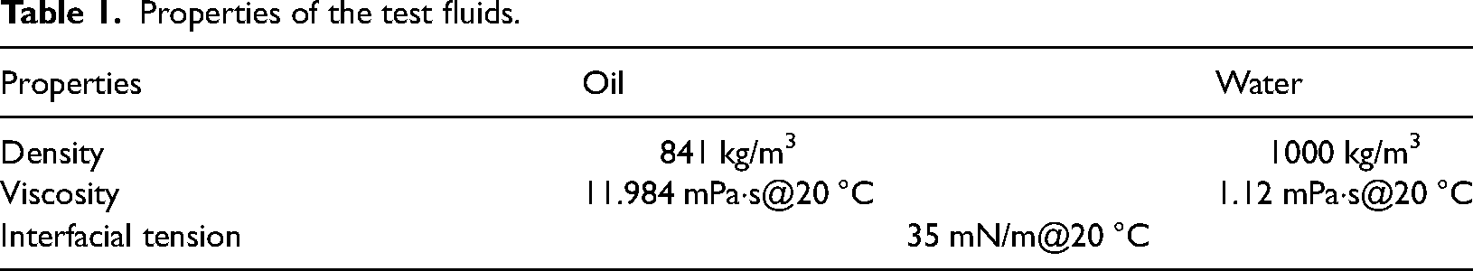
The schematic of the experimental setup used in this study is shown in Figure 1. Oil and water were used as test fluids. The average properties of the fluids are given in Table 1.

Figure 1.

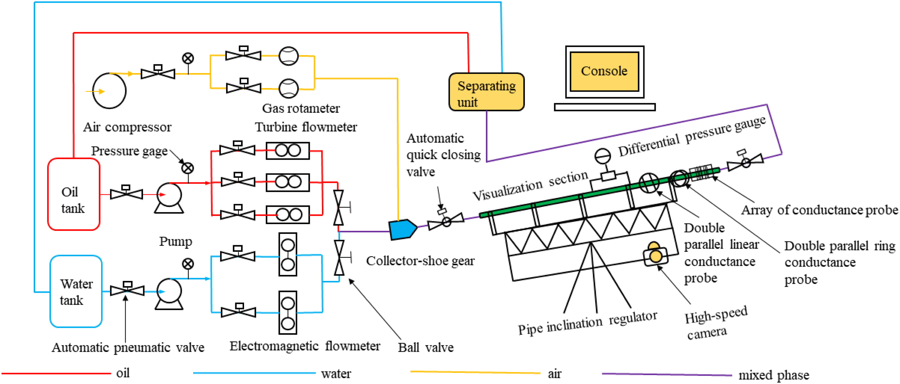
Diagram of the experimental setup.

Table 1.

Properties of the test fluids.

Properties	Oil	Water
Density	841 kg/m3	1000 kg/m3
Viscosity	11.984 mPa·s@20 °C	1.12 mPa·s@20 °C
Interfacial tension	35 mN/m@20 °C

The experimental setup is mainly composed of a water pipeline, oil pipeline, and visualization section. The oil pipeline had a pump, a pressure gauge, and three turbine flowmeters, with a maximum measurement capacity of 60 m³/d and a measure uncertainty of 1%. After being pumped and its turbine flowmeter measured, water flowed to the collector-shoe gear and then to the visualization section. The water pipeline had a pump, a pressure gauge, and two electromagnetic flowmeters, with a maximum measurement capacity of 60 m³/d and 1% uncertainty of the measure. After the water and oil were pumped and measured, the mixed phase entered the collector-shoe gear, then the two-phase flow was produced. The visualization section was composed of a PMMA tube and a series of measuring instruments, which can be adjusted from 0° to 90°. The PMMA tube was 6 m and its inner diameter was 20 mm. Movies of the flow were recorded by the high-speed camera, a SpeedCam MacroVis EoSens, with the highest speed of 285,000 fps.

In the experiment, the mixture velocity, water cut, and pipe inclination angle are given by the console. Before the injection of two-phase flow in each experiment, pure water is used to wash the pipe at high speed to ensure that there is no oil drop on the pipe wall. The experiment begins by injecting oil and water from individual tanks, which are mixed through a series of instruments into the pipe. The console shows that the flow rate is stable. It will take another 5 min for the flow to stabilize. When the flow stabilized, the high-speed camera and the pressure gauge begin to record the corresponding data at the same time, and the pressure gauge records the interval of 1 min. When the high-speed camera and the pressure gauge have measured the data, the automatic quick-closing valve will be closed. Finally, the mixture is collected and sorted, and the volume fraction of oil and water is measured.

Experimental results

The flow pattern map obtained in the experimental system described above is presented in Figure 2 in terms of oil and water superficial velocities. In pipes with inclination angles ( $\theta$ ) of +5° and +10°, the transition boundary between stratified flow and dual continuous flow occurs from oil superficial velocity ( ${\mu }_{so}$ ) of 0.30 up to 0.52 m/s and between ${\mu }_{so}$  = 0.15 and 0.35 m/s, respectively. Transition is considered to have happened when the interfacial wave appears to break and the first drops of one phase appear in the opposite phase. As expected, the water velocity required to break the interface and form drops decreases as the oil velocity increases.

Figure 2.

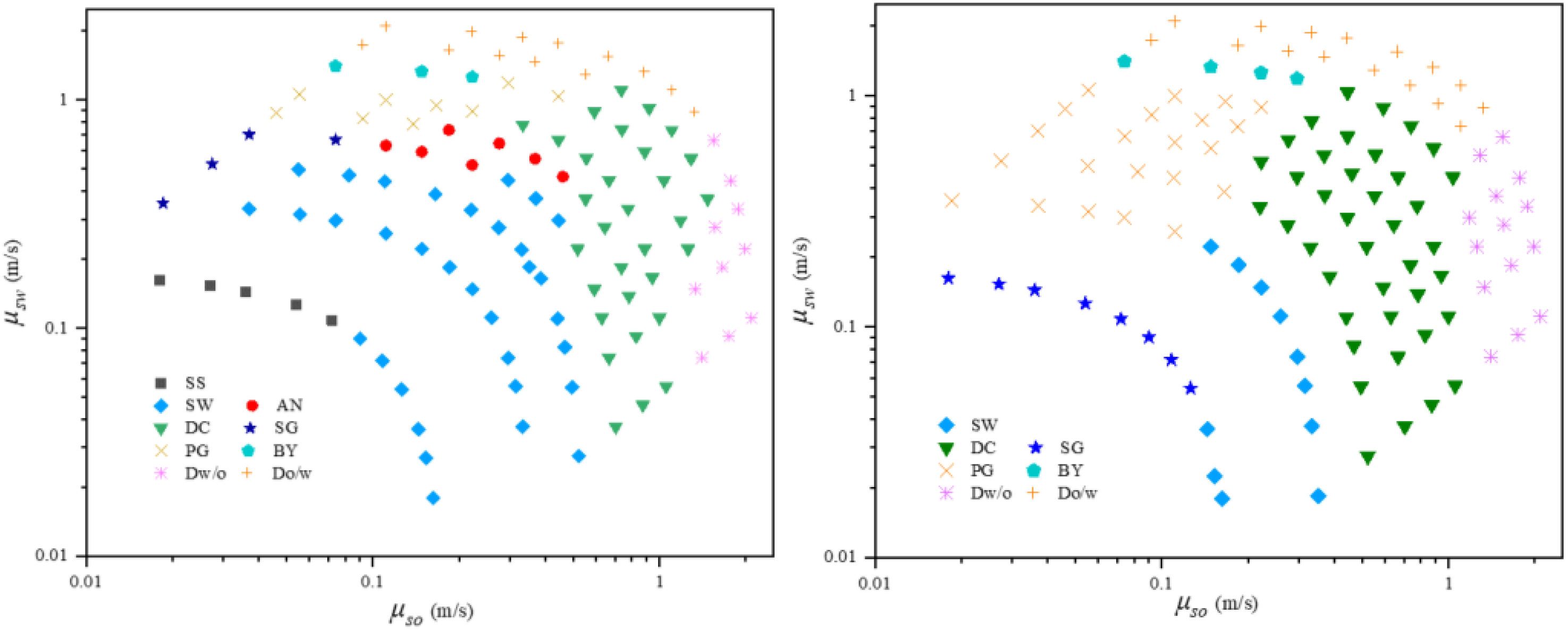
Flow pattern map for oil–water flow for pipe inclination angles of +5° (a), +10° (b). Flow patterns: Stratified smooth (SS), stratified wavy (SW), annular (AN), dual continuous (DC), slug (SG), plug (PG), bubble (BY), dispersion of water in oil (Dw/o), dispersion of oil in water (Do/w).

The visual observation and the analysis of the pictures showed clearly that the probability of stratified flow is reduced and drops more easily form with the increase of the pipe inclination angle. Stratified smooth (SS) and annular (AN) patterns disappear when the pipe inclination angle is +10°. At ${\mu }_{so}$  = 0.018 to 0.45 m/s and $\theta$  =  + 5°, AN, slug (SG), or plug (PG) patterns form as the water velocities increase instead of the dual continuous pattern. With the increase of the pipe inclination angle, more SG or PG patterns form as the water velocities increase. This could be attributed to the increase of turbulence as the water velocities increase, the oil layer is broken. In addition, with an increasing pipe inclination angle, the slip velocity and slip ratio of oil–water increase and form oil drops. Therefore, the continuous oil phase is more prone to discontinuities, and drops of the oil phase are more likely to form as the increase of water velocity and pipe inclination angle.

At higher oil velocity, interfacial waves break and drops form as the water velocity increases. This is due to the increase in the amplitudes and the decrease in the wavelength of interfacial waves, the interfacial waves become sharper. In addition, some water phases may touch the upper wall, and AN patterns form at a small pipe inclination angle.

The transition boundary diagram obtained in the experimental system is presented in Figure 3 in terms of oil and water superficial velocities at different pipe inclination angles. The separated flow is distributed inside the transition boundary and the non-separated flow is distributed on the opposite side. The transition boundary of pipe inclination angles with 0° and +5° basically coincide between ${\mu }_{so}$  = 0.15 and 0.35 m/s. The range of separated flow is obviously reduced with the increase of pipe inclination angles. Thus, it can be seen that the pipe inclination angle has a significant effect on the transition boundary.

Figure 3.

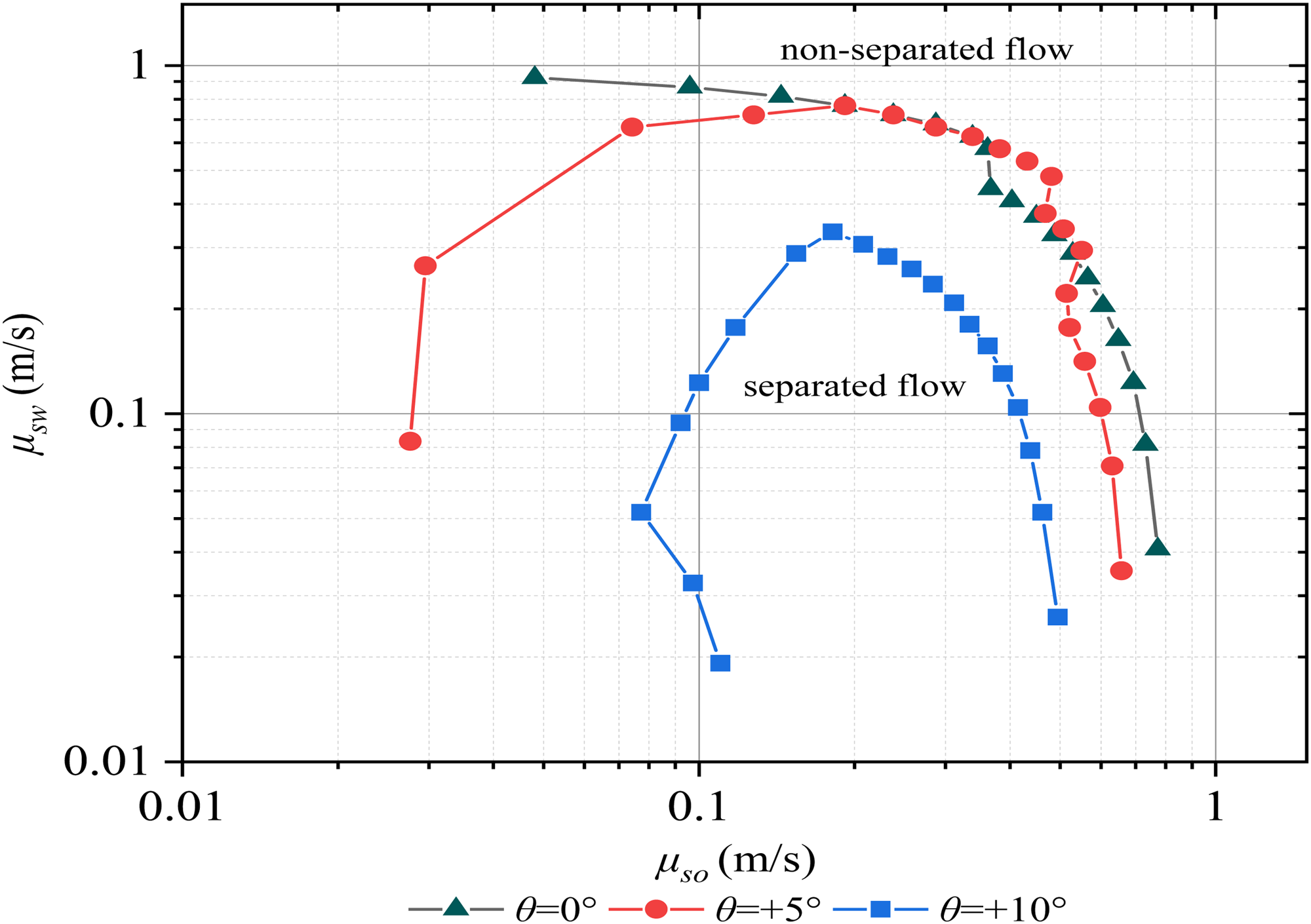
Transition boundary diagram of separated flow and non-separated flow at different pipe inclination angles.

The transition between stratified and double continuous oil–water flow

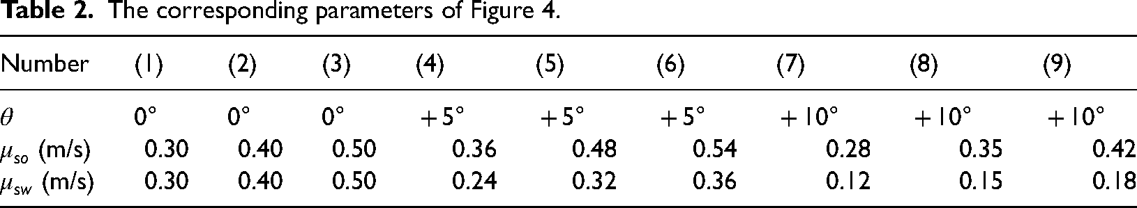
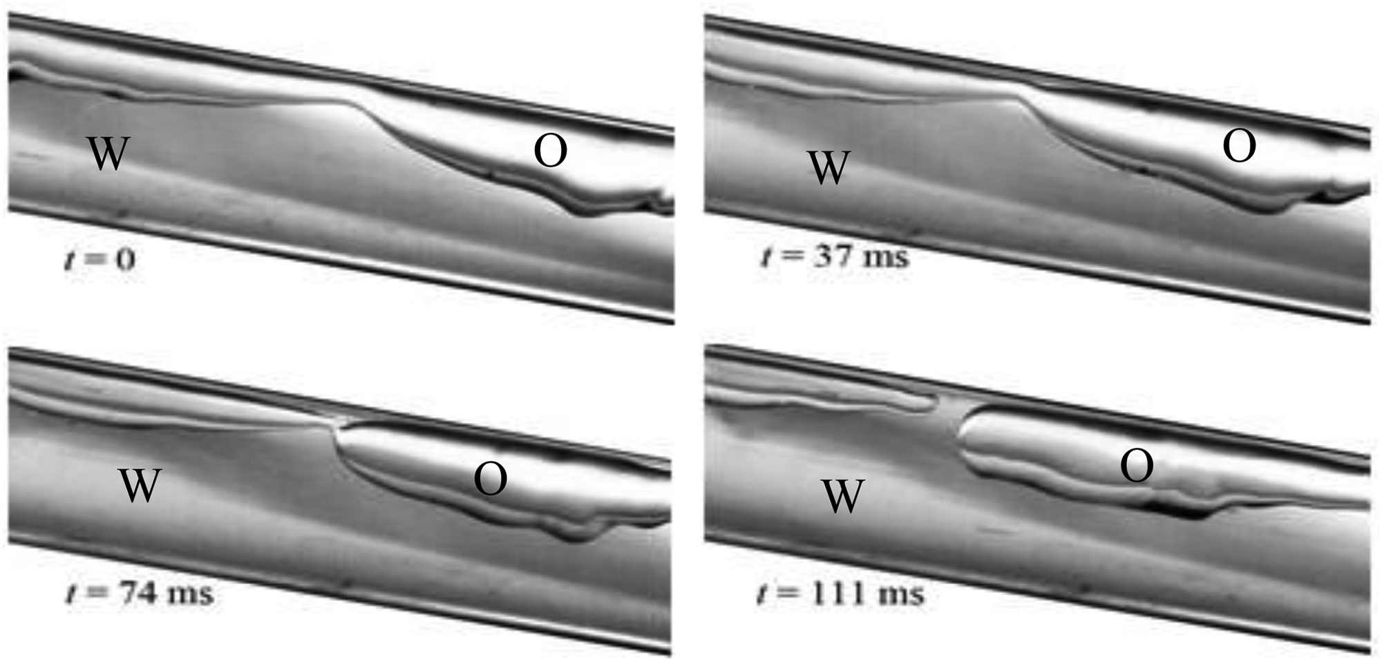
The effect of changing oil superficial velocity, water superficial velocity, and pipe inclination angle, where the transition to dual continuous flow occurs, is shown in Figure 4. The corresponding parameters of Figure 4 are listed in Table 2. The visual observation showed clearly that drop form as the oil and water superficial velocities. In addition, wave amplitude increases as the pipe inclination angle increases.

Figure 4.

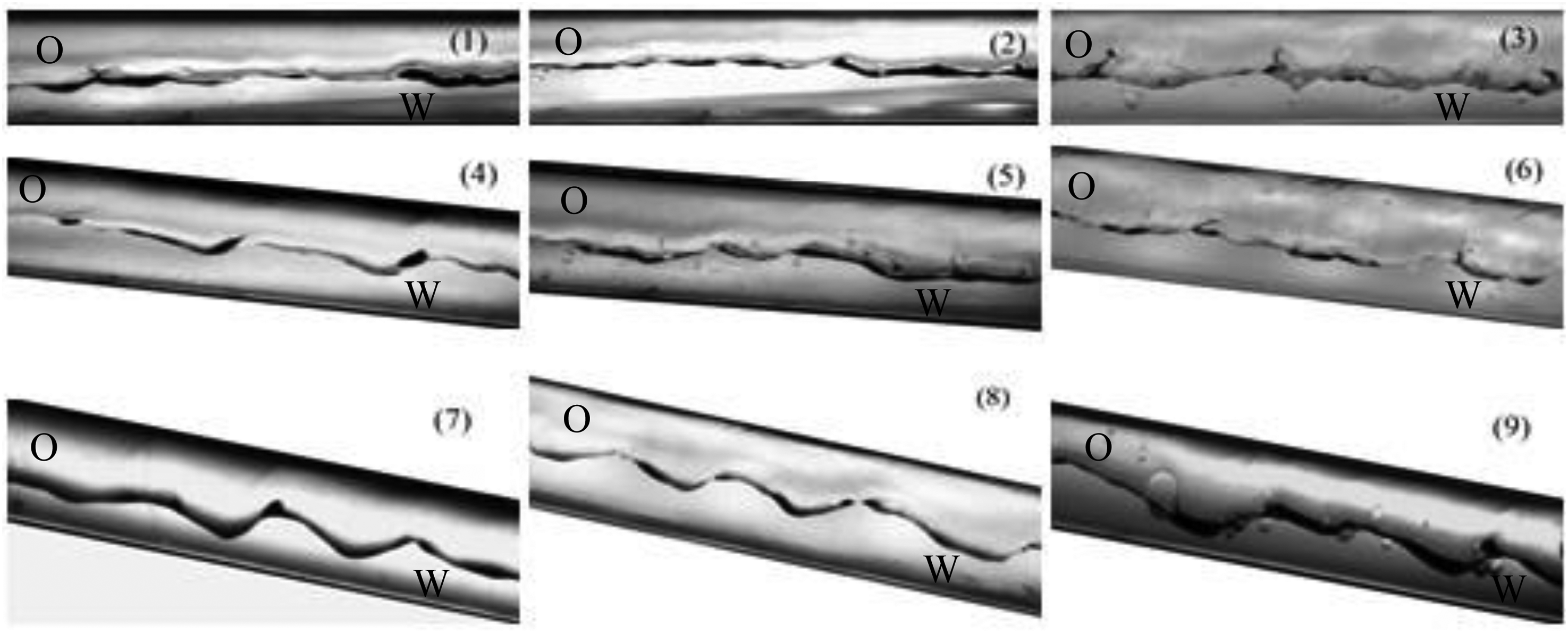
Transition from stratified to dual continuous flow. The flow direction is from right to left. Oil is labeled O and water is labeled W in the image.

Table 2.

The corresponding parameters of Figure 4.

Number	(1)	(2)	(3)	(4)	(5)	(6)	(7)	(8)	(9)
$\theta$	0°	0°	0°	+ 5°	+ 5°	+ 5°	+ 10°	+ 10°	+ 10°
${\mu }_{so}$ (m/s)	0.30	0.40	0.50	0.36	0.48	0.54	0.28	0.35	0.42
${\mu }_{sw}$ (m/s)	0.30	0.40	0.50	0.24	0.32	0.36	0.12	0.15	0.18

The transition between stratified and double continuous flow is considered to have happened when the first drops of one phase appear in the opposite phase. The stability of stratified flow is influenced by interfacial tension, gravity, inertia force, turbulent pulse dynamics, and oil–water slip velocity. Turbulent pulse dynamics, oil–water slip velocity, and gravity components are unstable factors. In order to predict the transition boundary, dimensionless numbers (Weber number, Reynolds number, and Froude number) were used: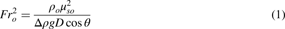

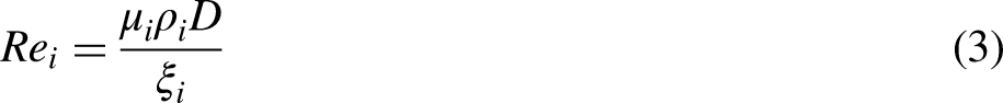
$$F{r}_o^2={\displaystyle \frac{{\rho }_o{\mu }_{so}^2}{\mathrm{\Delta }\rho gD\cos \theta }}$$

(1)

$$W{e}_w={\displaystyle \frac{{\rho }_w{\mu }_{sw}^{2}D}{\sigma }}$$

(2)

$$R{e}_i={\displaystyle \frac{{\mu }_i{\rho }_{i}D}{{\xi }_i}}$$

(3)

where $F{r}_o$ is the Froude number of the oil phase, $W{e}_w$ is the Weber number of the water phase, D is the inside diameter of the pipe, $\sigma$ is the surface tension force coefficient, $Re$ is the Reynolds number, i represents the respective phase, $\xi$ is the phase viscosity, and ${\mu }_i$ is the phase real velocities.

The Froude number of the oil phase is the ratio of inertial force to buoyancy force, which reflects the ability of the oil to overcome buoyancy and disperse in water. The Weber number of the water phase reflects the influence of oil–water interfacial tension on the transition boundary of stratified flow. The Reynolds number is the ratio of inertial force to wall friction force.

The Kutadelaze number is given by

$$Ku=(W{e}_{w}F{r}_o^2{)}^{0.25}={\mu }_m[C_w(1-C_w){]}^{0.5}{\left({\displaystyle \frac{{\rho }_o{\rho }_w}{\mathrm{\Delta }\rho g{\mu }_w\cos \theta }}\right)}^{0.25}$$

(4)

where $Ku$ is the Kutadelaze number, ${\mu }_m$ is the mixture velocity of oil–water, $C_w$ is the water holdup, and ${\mu }_w$ is the water real velocity.

By analyzing the transition boundary between stratified and dual continuous flow obtained in the experiment, there is a correlation between the Kutadelaze number and the Reynolds number. By using the experimental data to carry out regression, the parabolic relationship between the Kutadelaze number and the ratio of the oil and water Reynolds number at different pipe inclination angles is shown in Figure 5. The relationship between the Kutadelaze number and the Reynolds number can predict the transition boundary between stratified and dual continuous flow at different pipe inclination angles.

Figure 5.

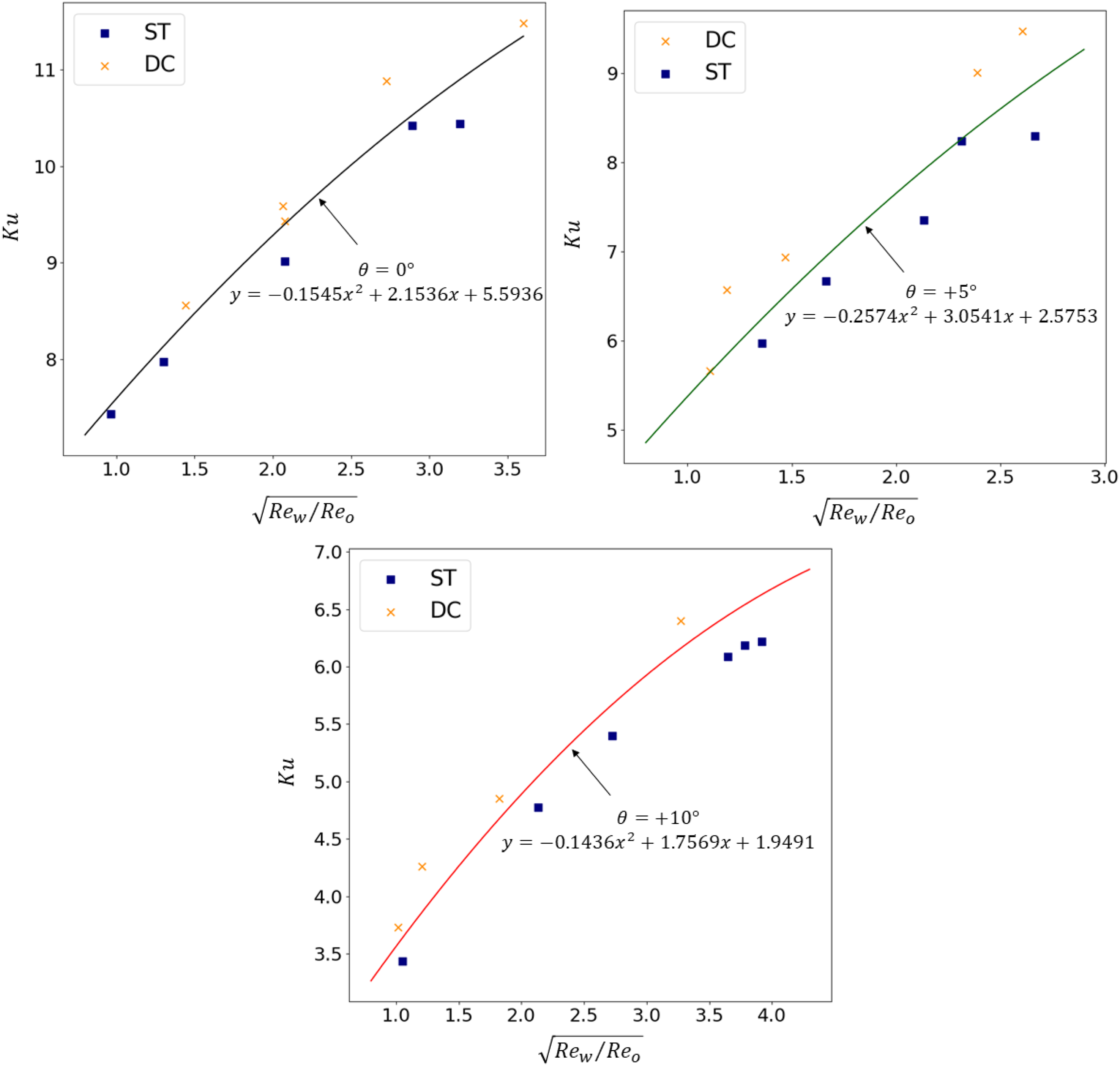
The predicted boundary and experimental data of transition between stratified and dual continuous flow at different pipe inclination angles. Flow patterns: Stratified flow (ST).

The mechanism of drop formation and prediction equation

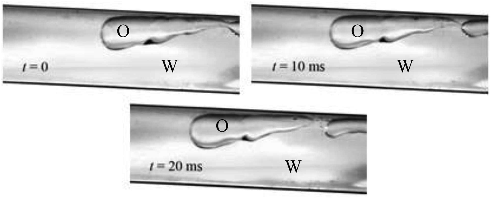
The flow images recorded by a high-speed camera at different pipe inclination angles, where the interfacial wave is not deformed (left column) and drop form (right column), are shown in Figure 6. The effect of changing superficial velocities of oil and water at $\theta$  =  +5°, where wave deformation occurs, is shown in Figure 7. The effects of changing pipe inclination angles or superficial velocities of oil or water, where drop formation or wave deformation occurs, are shown in experimental flow images, respectively.

Figure 6.

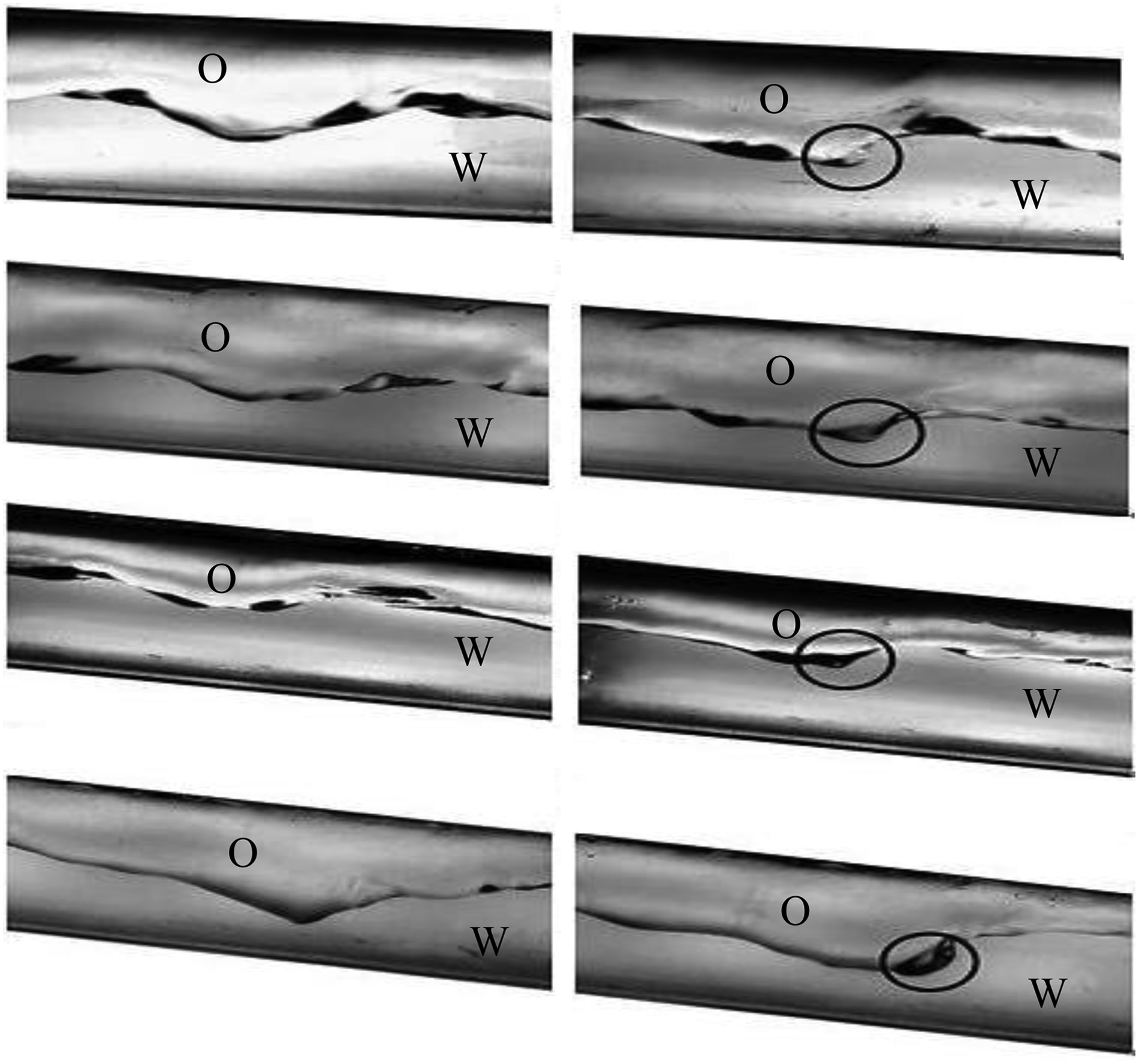
Flow images recorded by a high-speed camera: The interfacial wave before deformation (left column) and drop form (right column). The flow direction is from right to left. Oil is labeled O and water is labeled W in the image.

Figure 7.

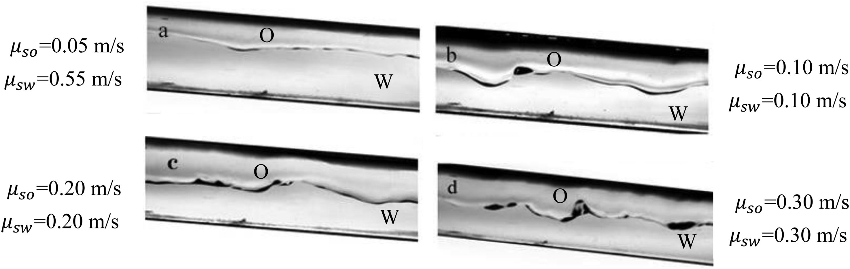
Wave deformation caused by changes in the superficial velocities of oil and water at pipe inclination angles with +5°. The flow direction is from right to left. Oil is labeled O and water is labeled W in the image.

Mechanism of drop formation

The mechanism of drop formation in the inclined pipe is slightly different from that in the horizontal pipe. The effects of gravity and buoyancy need to be considered. Kelvin–Helmholtz (KH) instability will cause the wavy disturbance on the oil–water interface to grow in amplitude while the component of gravity and interfacial tension will tend to stabilize it. When the destabilizing forces are greater than the stabilizing ones, interfacial wave deformation and drop formation occur. Interfacial waves will continue to grow, drops will eventually detach.

Analysis of interfacial waveform before and after deformation

Interfacial waves become unstable due to KH instability. The experimental observations showed that the interfacial wave before deformation conforms to the sinusoidal wave characteristic in the flow direction. The experimental precision measurements showed that the deformed interfacial wave can be characterized by two sine functions, which was divided into two parts: Stretched wave (w₁) and compressed wave (w₂).

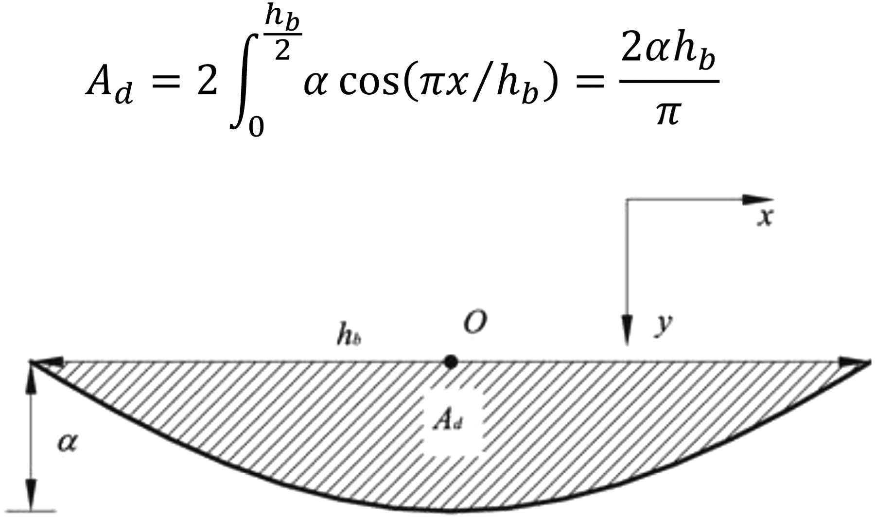
When a wave is stable, the two-dimensional wave in the flow direction (z-axis) is a sine wave and that in the vertical flow direction (x-axis) is a cosine wave (see Figure 8). The wave equations (equations (5) and (6)) can be expressed by

$$y=-\alpha \sin \left({\displaystyle \frac{2\pi z}{\lambda }}\right),\left(z|-{\displaystyle \frac{\lambda }{2}\le x\le 0}\right)$$

(5)

$$y=-\alpha \cos \left({\displaystyle \frac{\pi x}{h_b}}\right),\left(x|-{\displaystyle \frac{h_b}{2}\le x\le {\displaystyle \frac{h_b}{2}}}\right)$$

(6)

where $\alpha$ is the wave amplitude, $\lambda$ is the wavelength of the undeformed two-dimensional interfacial wave in the flow direction, and $h_b$ is the half wavelength of the undeformed two-dimensional interfacial wave in the vertical flow direction.

Figure 8.

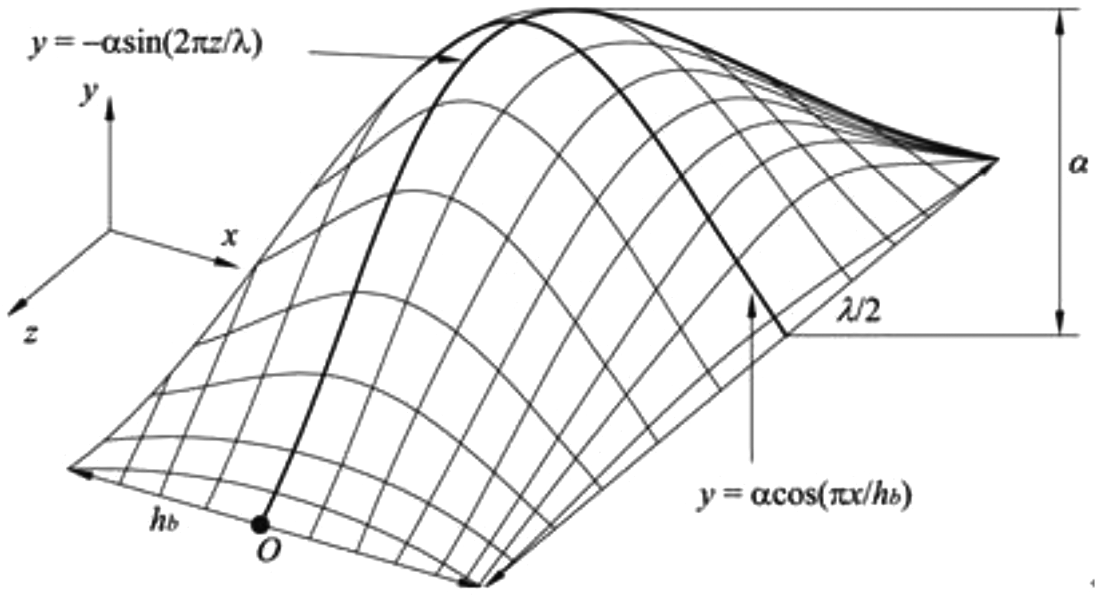
Three-dimensional undeformed waveform on the oil–water interface. Adapted from Holowach et al. (2002).

When the wave is deformed, the two-dimensional wave in the flow direction is made up of two sine waves (see Figure 9). The sum of the wavelength of the deformed waves is equal to the wavelength of the sinusoidal wave, the wave amplitude does not change. The wave equations (equations (8) and (9) can be expressed by

$$y=-\alpha \sin \left({\displaystyle \frac{2\pi z}{m\lambda }}\right),\left(z|-{\displaystyle \frac{m\lambda }{4}\le x\le 0}\right)$$

(7)

$$y=-\alpha \sin \left({\displaystyle \frac{2\pi z}{(2-m)\lambda }+{\displaystyle \frac{\pi }{2-m}}}\right),\left(z|-{\displaystyle \frac{\lambda }{2}\le x\le -{\displaystyle \frac{m\lambda }{4}}}\right)$$

(8)

where m is the ratio of the wavelength of stretched interfacial wave (w₁) to that of a sinusoidal wave.

Figure 9.

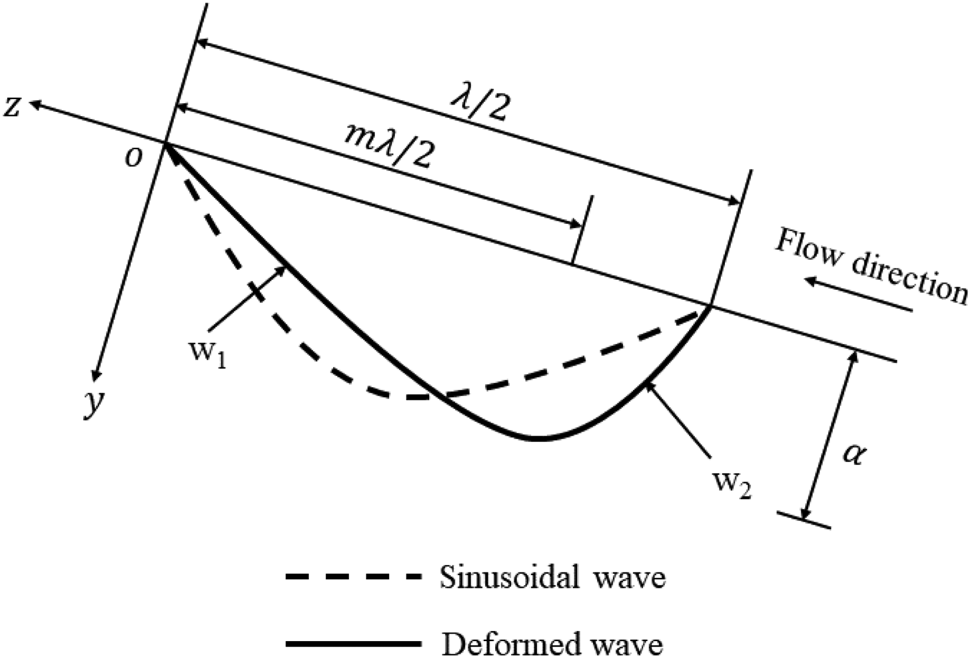
Two-dimensional deformed waveform on the oil–water interface. Adapted from Al-Wahaibi et al. (2007).

Interfacial wave force balance analysis

The force balance on a deformed two-dimensional interfacial wave in the flow direction is illustrated in Figure 10. The drag, buoyancy, gravitational, and surface tension forces are assumed to act on the whole wave. For entrainment to occur, it is assumed that the destructive force (drag force and component of gravity) should exceed the resisting force (component of surface tension force and buoyancy force):

$$\overrightarrow{F_{\sigma }}\cos \gamma +\overrightarrow{F_b}\sin \theta -\overrightarrow{F_d}-\overrightarrow{G}\sin \theta \le 0$$

(9)

where $\overrightarrow{F_{\sigma }}$ is the surface tension force, $\overrightarrow{F_b}$ is the buoyancy force, $\overrightarrow{F_d}$ is the drag force, $\overrightarrow{G}$ is the gravitational force, and $\gamma$ is the angle between the surface tension force and the flow direction.

Figure 10.

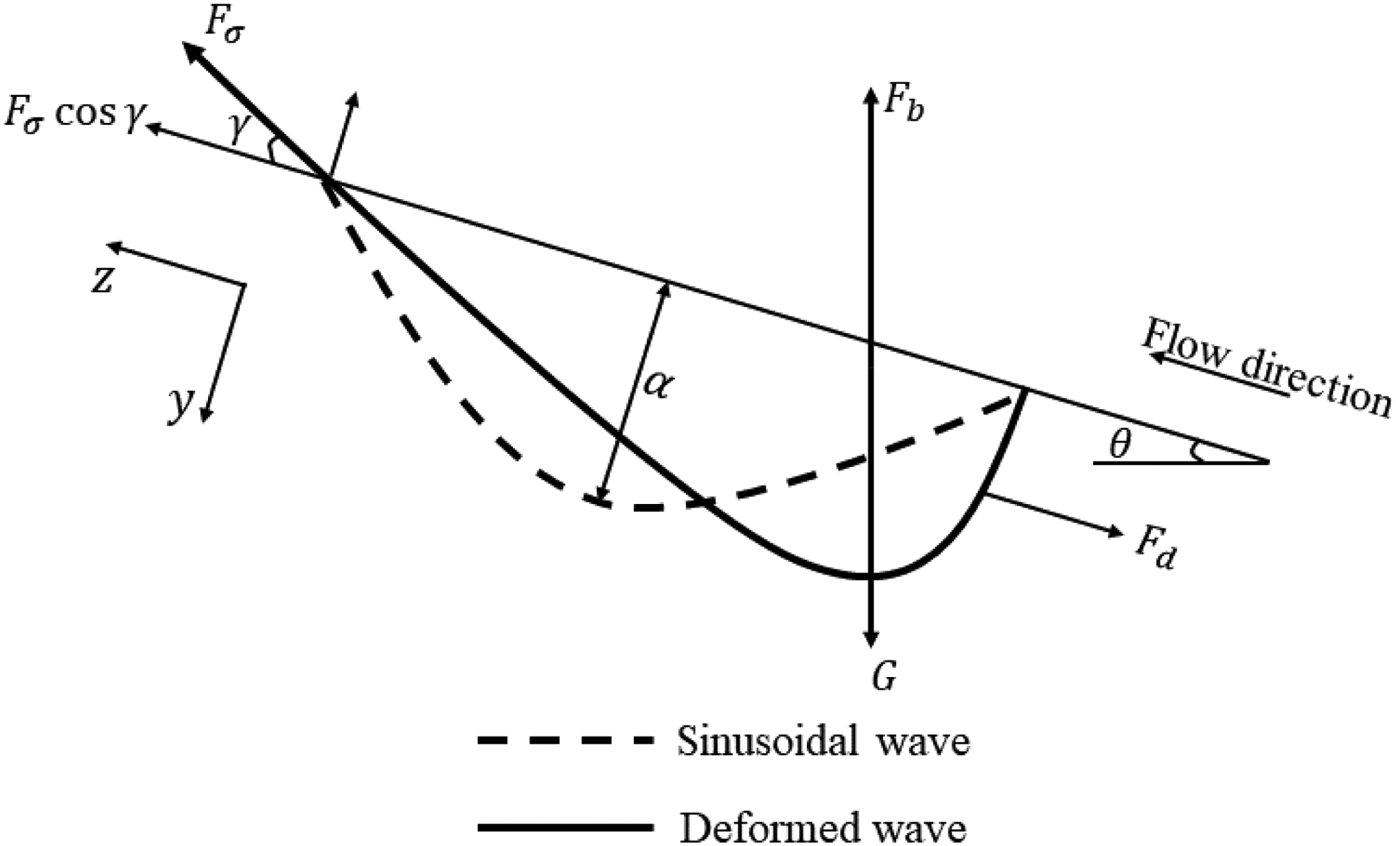
Force balance on a deformed two-dimensional wave on the oil–water interface. Adapted from Al-Wahaibi et al. (2007).

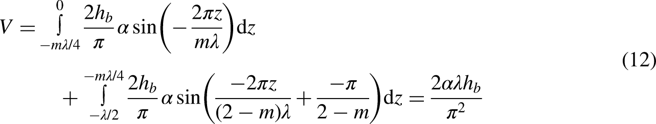
The resultant force (the buoyancy force and the gravitational force) calculation is given as

$$F_b-G={\rho }_{w}gV-{\rho }_{o}gV$$

(10)

where V is the volume of the interfacial wave.

From equations (6), (8), and (9), the volume of the sinusoidal wave (equation (11)) and that of the deformed wave (equation (12)) are calculated by the integral:

$$V=\underset{0}{\overset{\lambda /2}{\int }}{\displaystyle \frac{2h_b}{\pi }\alpha \sin (2\pi z/\lambda )\mathrm{d}z={\displaystyle \frac{2\alpha \lambda h_b}{{\pi }^2}}}$$

(11)

$$\begin{array}{rl}V=& \underset{-m\lambda /4}{\overset{0}{\int }}{\displaystyle \frac{2h_b}{\pi }\alpha \sin \left(-{\displaystyle \frac{2\pi z}{m\lambda }}\right)\mathrm{d}z}\\ & +\underset{-\lambda /2}{\overset{-m\lambda /4}{\int }}{\displaystyle \frac{2h_b}{\pi }\alpha \sin \left({\displaystyle \frac{-2\pi z}{(2-m)\lambda }+{\displaystyle \frac{-\pi }{2-m}}}\right)\mathrm{d}z={\displaystyle \frac{2\alpha \lambda h_b}{{\pi }^2}}}\end{array}$$

(12)

So, the volume of the interfacial waves before and after deformation is constant.

Drag force calculation

In the process of interfacial wave deformation, the drag force plays a destructive role. The direction of the drag force is opposite to the flow direction (see Figure 10). The drag force is calculated by knowing the drag coefficient, the effective area normal to the flow on which it acts, and the relative velocities between the two phases. The drag force is given by

$$F_d=C_d{A}_d{\rho }_w{\displaystyle \frac{{({\mu }_w-{\mu }_o)}^2}{2}}$$

(13)

where $C_d$ is the drag coefficient, $A_d$ is the cross-sectional wave area normal to the flow, and ${\mu }_o$ is the velocity of oil.

To calculate the drag coefficient $C_d$ , the results are used. They related the drag coefficient to slower and faster phase Reynolds numbers, viscosities, and densities of upper and lower phases from a wide range of experimental data. The following correlation for the drag coefficient was finally suggested:

$$C_d=286R{e}_{\mathrm{slower}\mathrm{phase}}^{1/6}R{e}_{\mathrm{faster}\mathrm{phase}}^{-2/3}{\left({\displaystyle \frac{{\rho }_{\mathrm{upper}\mathrm{phase}}}{{\rho }_{\mathrm{lower}\mathrm{phase}}}}\right)}^{1/3}\times {\left({\displaystyle \frac{{\xi }_{\mathrm{upper}\mathrm{phase}}}{{\xi }_{\mathrm{lower}\mathrm{phase}}}}\right)}^{-2/3}$$

(14)

where $R{e}_{\mathrm{slower}\mathrm{phase}}$ is the Reynolds number of the slower phase, $R{e}_{\mathrm{faster}\mathrm{phase}}$ is the Reynolds number of the faster phase, ${\rho }_{\mathrm{upper}\mathrm{phase}}$ is the upper (oil) phase density, ${\rho }_{\mathrm{lower}\mathrm{phase}}$ is the lower (water) phase density, ${\xi }_{\mathrm{upper}\mathrm{phase}}$ is the oil phase viscosity, and ${\xi }_{\mathrm{lower}\mathrm{phase}}$ is the water phase viscosity.

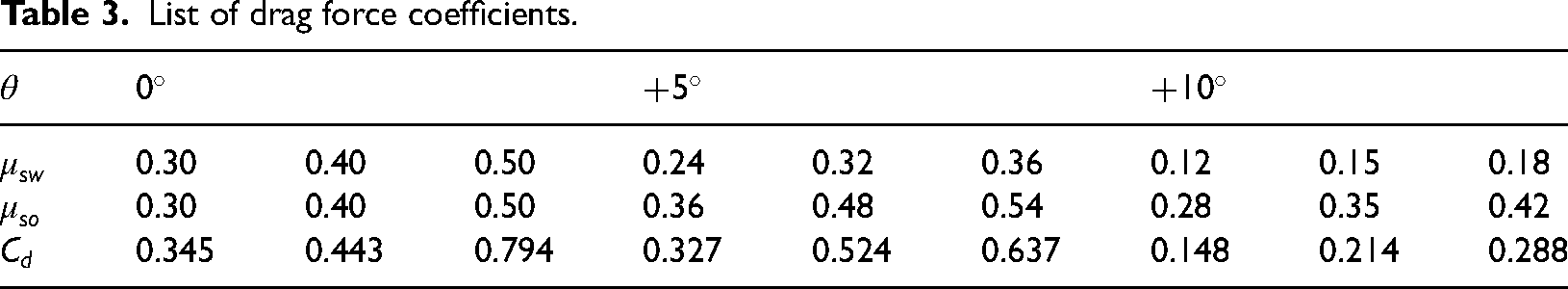
The drag coefficients calculated from the experimental data are listed in Table 3.

Table 3.

List of drag force coefficients.

$\theta$	$0^{\circ }$			$+5^{\circ }$			$+{10}^{\circ }$
${\mu }_{sw}$	0.30	0.40	0.50	0.24	0.32	0.36	0.12	0.15	0.18
${\mu }_{so}$	0.30	0.40	0.50	0.36	0.48	0.54	0.28	0.35	0.42
$C_d$	0.345	0.443	0.794	0.327	0.524	0.637	0.148	0.214	0.288

The area of drag force is shown in Figure 11. From equation (7), the cross-sectional wave area normal to the flow is calculated by the integral:

$$A_d=2\underset{0}{\overset{h_b/2}{\int }}\alpha \cos (\pi x/h_b)={\displaystyle \frac{2\alpha h_b}{\pi }}$$

(15)

Figure 11.

Schematic diagram of the drag force area. Adapted from Holowach et al. (2002) and Ryu and Park (2011).

Based on the above, the drag force equation:

$$F_d=C_d{\displaystyle \frac{2\alpha h_b}{\pi }{\rho }_w{\displaystyle \frac{{({\mu }_w-{\mu }_o)}^2}{2}}}$$

(16)

Surface tension force calculation

In the process of interfacial wave deformation, the surface tension force plays a stabilizing role. The surface tension is given by

$$F_{\sigma }=\sigma K{A}_{\sigma }$$

(17)

where K is the interfacial curvature and $A_{\sigma }$ is the area of surface tension force.

The component of surface tension force is calculated by the integral: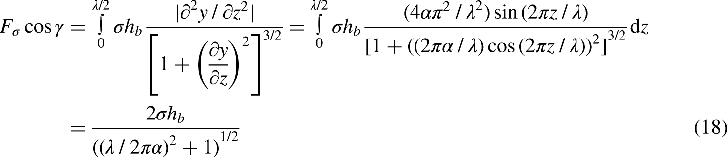

$$F_{\sigma }\cos \gamma =\underset{0}{\overset{\lambda /2}{\int }}\sigma h_b{\displaystyle \frac{|{\mathrm{\partial }}^{2}y/\mathrm{\partial }{z}^2|}{{\left[1+{\left({\displaystyle \frac{\mathrm{\partial }y}{\mathrm{\partial }z}}\right)}^2\right]}^{3/2}}=\underset{0}{\overset{\lambda /2}{\int }}\sigma h_b{\displaystyle \frac{(4\alpha {\pi }^2/{\lambda }^2)\sin (2\pi z/\lambda )}{{[1+{((2\pi \alpha /\lambda )\cos (2\pi z/\lambda ))}^2]}^{3/2}}\mathrm{d}z={\displaystyle \frac{2\sigma h_b}{{({(\lambda /2\pi \alpha )}^2+1)}^{1/2}}}}}$$

(18)

For the wave to deform

$$F_{z1}=\overrightarrow{F_{\sigma }}\cos \gamma +\overrightarrow{F_b}\sin \theta -\overrightarrow{F_d}-\overrightarrow{G}\sin \theta \le 0$$

(19)

where $F_{z1}$ is the resultant force of the interfacial wave in the flow direction.

From equations (10), (16), and (18), for drop formation equation (20) becomes:

$${\displaystyle \frac{2\sigma h_b}{{({(\lambda /2\pi \alpha )}^2+1)}^{1/2}}+({\rho }_w-{\rho }_o)g{\displaystyle \frac{2\alpha \lambda h_b}{{\pi }^2}\sin \theta -C_d{\displaystyle \frac{2\alpha h_b}{\pi }{\rho }_w{\displaystyle \frac{{({\mu }_w-{\mu }_o)}^2}{2}\le 0}}}}$$

(20)

where ${\mu }_o$ is the oil real velocity.

The same analysis can be applied to water waves and water drop formation.

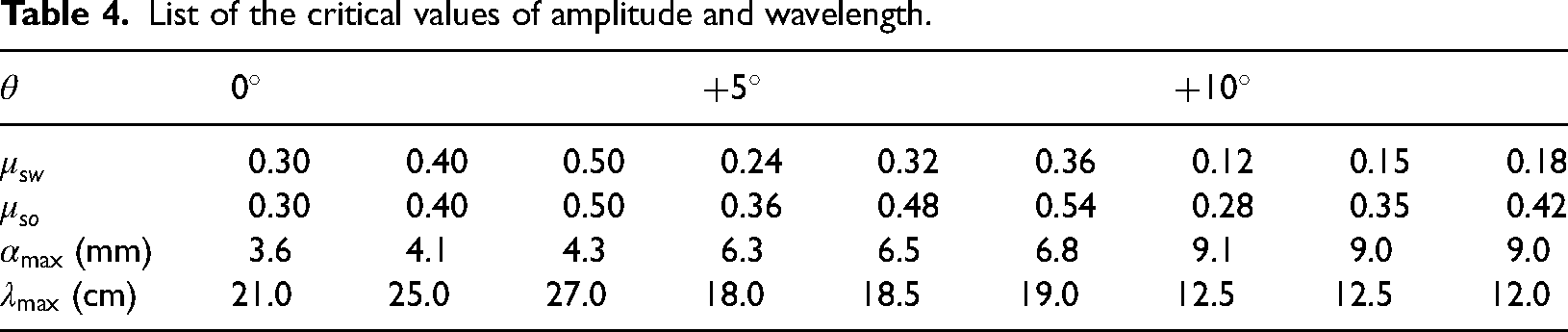
In addition, according to the entrainment equation (Equation (20)) and experimental data, the comparative results of critical wavelengths are shown in Figure 12. The experimental values are close to the predicted ones. The comparative results of critical amplitude are consistent with those of critical wavelengths. It shows that the prediction equation can better predict the drop entrainment. In addition, the critical values of amplitude and wavelength are shown in Table 4.

Figure 12.

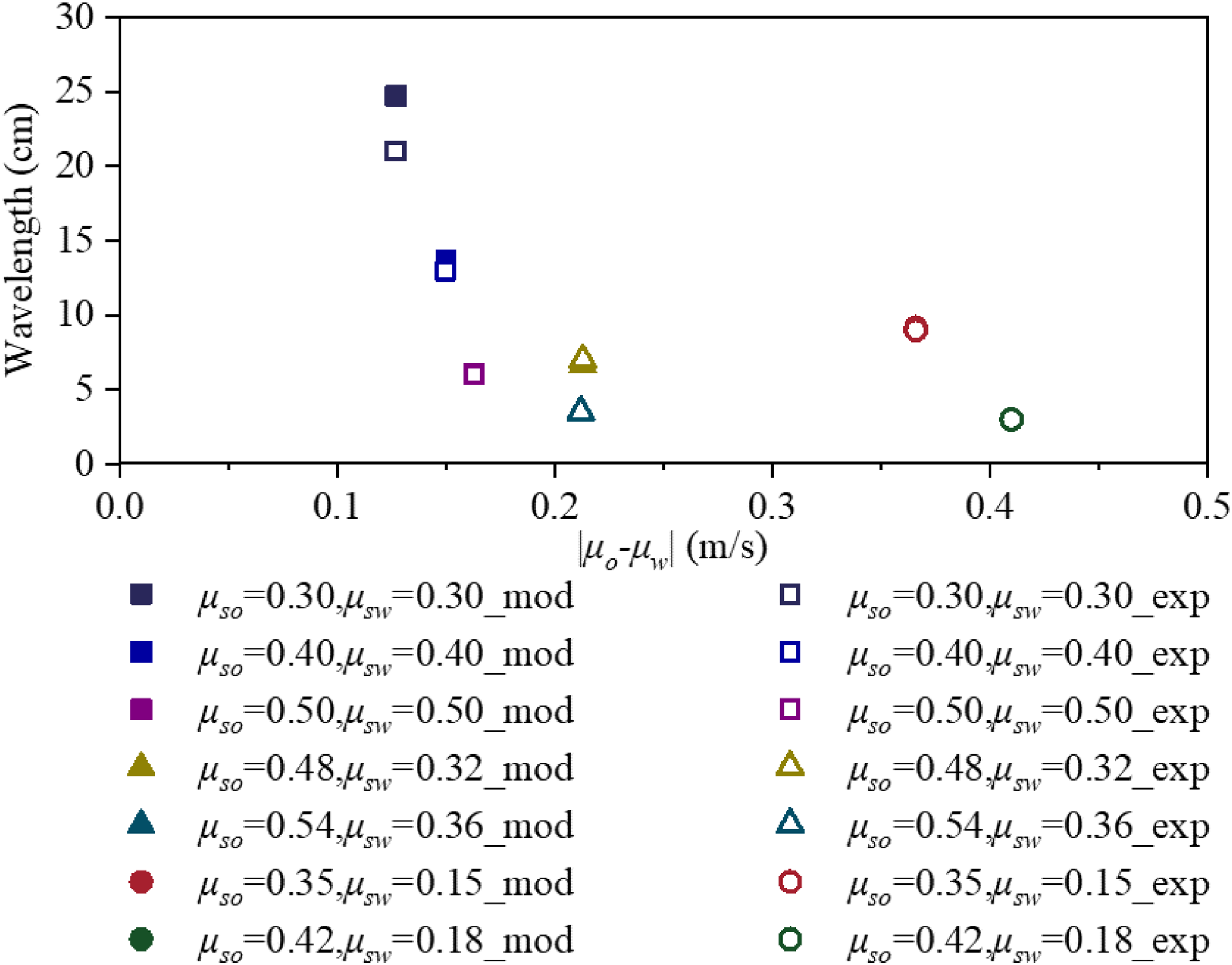
Comparison between predicted and experimental critical wavelengths at the six selected entrainment onset velocities and different pipe inclination angles. All the superficial velocities are in m/s.

Table 4.

List of the critical values of amplitude and wavelength.

$\theta$	$0^{\circ }$			$+5^{\circ }$			$+{10}^{\circ }$
${\mu }_{sw}$	0.30	0.40	0.50	0.24	0.32	0.36	0.12	0.15	0.18
${\mu }_{so}$	0.30	0.40	0.50	0.36	0.48	0.54	0.28	0.35	0.42
${\alpha }_{max}(\mathrm{mm})$	3.6	4.1	4.3	6.3	6.5	6.8	9.1	9.0	9.0
${\lambda }_{\max }(\mathrm{cm})$	21.0	25.0	27.0	18.0	18.5	19.0	12.5	12.5	12.0

The transition between separated and intermittent oil–water flow

The transition between AN and PG flow occurs at a small pipe inclination angle and higher water holdup, the transition between stratified and PG flow occurs at a wide pipe inclination angle and lower water holdup, are shown in Figures 13 and 14.

Figure 13.

Transition from stratified to plug flow at ${\mu }_{so}$  = 0.15 m/s, ${\mu }_{sw}$  = 0.30 m/s, $\theta$  =  + 10°. The flow direction is from right to left. Oil is labeled O and water is labeled W in the image.

Figure 14.

Transition from annular to plug flow at ${\mu }_{so}$  = 0.10 m/s, ${\mu }_{sw}$  = 0.70 m/s, $\theta$  =  + 3°. The flow direction is from right to left. Oil is labeled O and water is labeled W in the image.

The density difference between oil and water is small, and oil is more likely to invade the water phase in the inclined pipe, forming the interfacial wave with a larger amplitude, the area of the oil phase is reduced. When the water holdup is high, the transition to intermittent flow is caused by oil phase discontinuity. However, for the transition to occur, a large two-phase velocity difference is required when the oil phase cross-section area is large. The transition boundary is influenced by pipe inclination angle, oil–water slip velocity, and water holdup. The Froude number and Weber number were modified to reflect the effects of these flow parameters.

Therefore, the Kutadelaze number is given by

$$Ku=(WeF{r}^2{)}^{0.25}={\left[{\displaystyle \frac{{\rho }_w{\mu }_w^{2}D}{\sigma \cos \theta }\times {\displaystyle \frac{{({\mu }_o-{\mu }_w)}^2}{g{\epsilon }_{w}D\cos \theta }}}\right]}^{0.25}$$

(21)

where ${\epsilon }_w$ is the water holdup.

The analysis of experimental data shows that there is an exponential relationship between the Kutadelaze number and the ratio of the oil and water Reynolds number. The regression of experimental data is shown in Figure 15. Therefore, the transition boundary between separated and intermittent oil–water flow is obtained.

Figure 15.

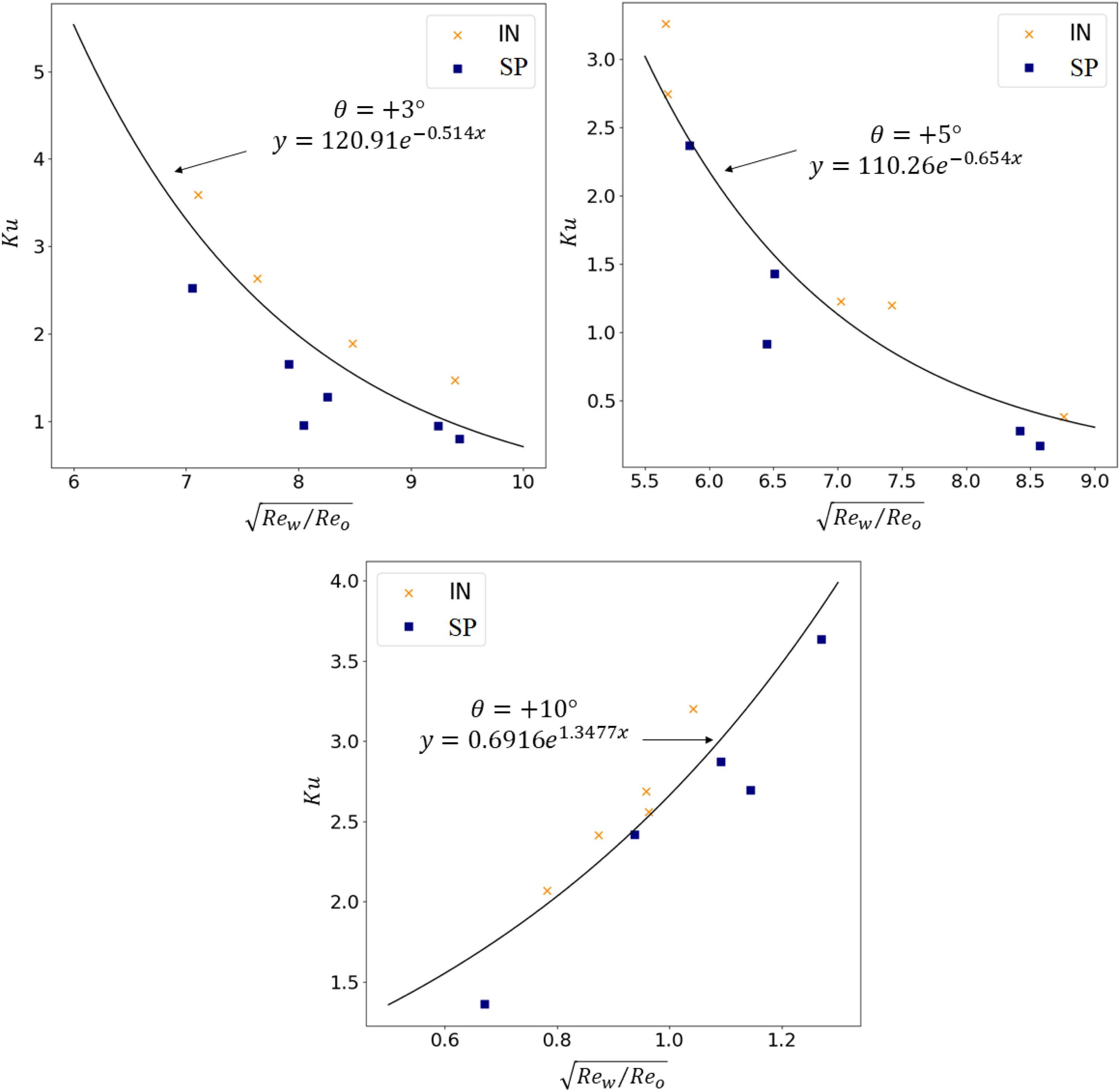
The predicted boundary and experimental data of transition between separated and intermittent oil–water flow at different pipe inclination angles. Flow patterns: Separated flow (SP) and intermittent flow (IN).

Conclusions

The transition boundaries between the separated and non-separated oil–water flow and the mechanism of drop formation were investigated in this study. The oil–water flow pattern maps and transition boundary diagrams of separated and non-separated at different pipe inclination angles were plotted according to the experimental data. The ranges of oil and water superficial velocities were determined when flow pattern transitions occur.

The dimensionless numbers (Weber number, Froude number, Reynolds number, and Kutadelaze number) were used to predict the transition boundaries between the stratified (or the separated flow) and the dual continuous flow (or the intermittent flow). The prediction equations of the transition boundary were obtained by regression of the experimental data.

The mechanism of drop formation was investigated by the interfacial wave force balance analysis. The four forces acting on the interfacial wave were calculated by integration. The resultant force in the parallel flow direction was calculated and the prediction equation was derived. By comparing experimental and predicted critical wavelengths, the prediction equation is proved to be correct.