Sage Journals: Discover world-class research

Abstract

This study endeavors to identify how urbanization and energy factors (use, prices, and policies) have influenced CO₂ emission patterns per capita among the 48 U.S. states and the District of Columbia from 2000 to 2015. To examine interconnections between state-level emissions, three different spatial panel data models are estimated: the spatial autoregressive model, spatial error model, and the spatial Durbin model models. This study makes contributions to the literature by applying a spatial panel data approach and including policies on urbanization and renewable standards. Urbanization is found to have a statistically significant, negative direct effect on emissions, yet a negative spillover effect such that a 1.0% increase in state i's urbanization level leads to a 0.30% decrease in its own state's emissions, but a 0.012% increase in an adjacent state j's emissions. Although state-level emissions are increased by higher energy use and coal consumption, both energy prices and renewable portfolio standards decrease emissions both within their own and adjacent states.

Keywords

spatial models energy urbanization

Introduction

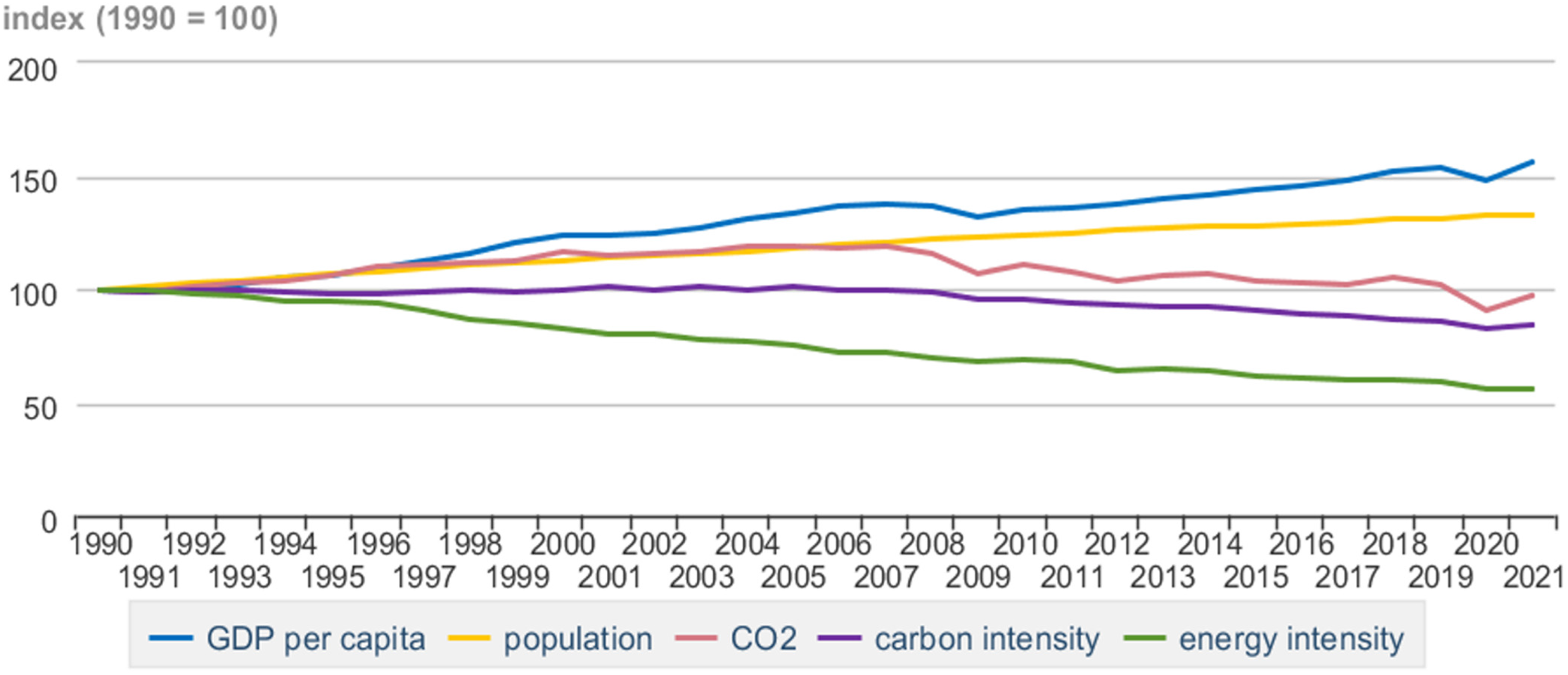
Due to concerns about global climate change, the public has an interest in policies that advocate limiting the rise of CO₂ emissions. Studies of urban environmental transition emphasize that urbanization can have both negative and positive effects on the environment making it difficult to determine the net effect a priori (Cole and Neumayer, 2004; Liddle and Lung, 2010). Examining the linkages among CO₂ emissions, urbanization, and other factors are significant as the United States is the second largest aggregate emitter globally from 2020 to 2050, based upon its share of global energy-related CO₂ emissions and global roadmap for building and construction (International Energy Agency [IEA], 2020). The availability of state-level data from EIA and the Carbon Dioxide Information Analysis Center (CDIAC) is the basic information required to study CO₂ emissions, urbanization, energy consumption, and socioeconomic variables in the United States (Figure 1). This research investigates how urbanization and other variables reflecting energy use impact carbon emissions in the United States.

Figure 1.

Trends in energy-related carbon dioxide emissions and key indicators in the U.S.

The principal forces driving the U.S. CO₂ emissions come from urbanization, transportation, coal-fired power plants, and energy use (Bekun, 2022; Mujtaba et al., 2022, Adedoyin et al., 2021; York et al., 2003; Aldy, 2005; Carson, 2010; Newman and Kenworthy, 1999; Gonzalez, 2009; Cole and Neumayer, 2004; Andrews, 2008; Davis et al., 2011; Tawfeeq et al., 2020; Ongan et al., 2022; Iwata et al., 2012; Burnett et al., 2013; Sadorsky, 2014; Shahbaz et al., 2017). Most previous studies have assumed that interjurisdiction regions are independent, thereby ignoring spatial interactions. However, one region's energy inputs often rely on neighboring regions. For example, urban areas in one state utilize electricity generated in another state. Thus, ignoring spatial dependence may lead to biased parameters when using an OLS approach to explain CO₂ emissions (Elhorst, 2009; Lesage and Pace, 2009; Baltagi et al., 2012). Spillover impacts resulting from spatial lags of CO₂ emissions across states include factors such as: (1) regionally distributed electricity from more than 3,200 fossil fuel–fired power plants in the U.S. (U.S. EIA, 2016); (2) urbanization and its impact on own state and neighboring state emissions; and (3) transportation of goods and its spillover effects of emissions across states.

Furthermore, a controversial discourse has recently advanced about the subject of whether CO₂ emissions measurement must be based upon space-related consumption or production method (Davis et al., 2011; Peters et al., 2011). Production-based accounting (PBA) of CO₂ emissions for fossil fuel consumption estimates the greenhouse gas emissions from all the coal, crude oil, and gas consumed in a state by power plants, residential, and industrial production of goods and services. While the PBA has several drawbacks. First, it excludes CO₂ emissions driving from international trade and transportation. Since such CO₂ emissions do not occur within a specific state, its impact on specific territories is complicated. Second, industries that are energy-intensive in states with CO₂ emission regulations and taxes may move into other states with fewer regulations and lower costs of energy. However, the goods and services produced in the less regulated states could then be exported to the more regulated states. Hence, reducing CO₂ emissions in one state might be directly correlated with rising CO₂ emissions in other states. Third, the CO₂ emission leakage from the outsource production of carbon-intensive goods to the United States is a reallocation of CO₂ emissions to states. Thus, one state's production can also be driven by consumption in other states. Consumption-based accounting (CBA) is an approach to consider these issues. It subtracts all CO₂ emissions that are incorporated in exported goods and services from states, including CO₂ emissions of transportation, and the contained CO₂ emissions in the inventories of the importing states (Aldy, 2005; Auffhammer and Carson, 2008; Peters et al., 2011; Tawfeeq et al., 2020). Hence, with respect to production-based inventories, low-emission states may be less clean in the CBA approach and high CO₂ emissions states could produce goods for the standard of living of low CO₂ emission states. Thus, previous research has found that CO2 emissions are primarily driven by city size, population, GDP, and an economy's energy consumption.

We utilized several complementary methods to investigate the problem in this study, arguing that the contradiction between urbanization and CO₂ emissions arises not only from different scales of analysis (i.e., state versus national) but also from limitations in how previous studies theorized and estimated the factors of CO2 emissions and urbanization. To address this shortcoming, we synthesize insights from nonspatial and spatial econometric methods to develop a framework for understanding how urbanization and energy factors affect CO₂ emissions across 48 states and District of Columbia in the United States. Hence, the spatial linkage is examined by determining spatial panel data models that are control for spatial impacts over time and space (LeSage and Pace, 2009; Aldy, 2005). Indeed, estimated parameters might be biased when spatial correlation is not considered.

Using spatial econometric models is an adequate approach to study the effects of urbanization, per-capita gross state product (GSP), energy use, energy prices, and coal consumption on CO₂ emissions by state level from 2000 to 2015. Additionally, the spatial reliance signifies that an energy policy implemented in one state could have spillover impacts in neighboring states (Kindle and Shawhan, 2011). The estimate of such spillovers is significant to determine the direct and indirect impacts of state-level policies adopted in the United States which affect the level of CO₂ emissions. Hence, this study attempts to control spatial correlation in estimating the impact of urbanization and other driving forces on CO₂ emissions.

In this context, the objective of this study is to examine the spillover impacts of changes in energy use and urbanization growth on CO₂ emissions in the US. More importantly, the main goal of this study is to provide a basic reference for inverters and policy makers to make proper decisions and set CO₂ emission reduction targets and policies.

This research makes novel contributions to literature through its use of a spatial panel data approach. More specifically, we have taken into consideration urbanization and energy-related factors on CO₂ emissions when examining state-level panel data for 2000–2015. This time period captures recent developments in state-level economic growth and energy use policies, like state-level passage of renewable portfolio standards (RPS). Moreover, this period covered pre-recession and post-recession of 2008 in the U.S. economy.

Theoretical model

Urban areas are the center of energy consumption and the consumption of fossil fuels in transportation, electricity, and industrial goods, all of which generate CO₂ emissions. However, many power plants and industrial firms are in rural regions and they burn fossil fuels—emitting a high amount of CO₂ and polluting the entire environment. It has been theoretically shown that an increase in energy use occurs in urban areas relative to higher economic activities and income levels (Canadell et al., 2007). Moreover, Itkonen (2012) assumes that energy consumption and income are linearly associated. Itkonen (2012) modifies the EEO model by examining the effect of income on CO₂ emissions when the consumption of energy has a positive linear relationship with income. Also, Jaforullah and King (2017) model CO₂ emissions, using the EEO approach to identify determinants of CO₂ emissions. The EEO model, although, indicates that energy consumption is a function of income; energy use and income are two critical exogenous variables of CO₂ emissions. However, based upon their model, they concluded that the consumption of energy was not an independent determinant of CO₂ emissions (Jaforullah and King, 2017).

We argue that energy consumption can be used as an independent variable to explain CO₂ emissions. First, most of the empirical studies on the relationships between energy use, GDP, and CO₂ emissions have included energy consumption as a main independent variable (Soytas et al., 2007; Martinez-Zarzoso and Maruotti, 2011; Wang, et al., 2011; Chuai et al., 2012; Tawfeeq et al., 2019; Sadorsky, 2014). This literature has focused on the linkages between CO₂ emissions, income, and energy consumption by utilizing energy use variables as explanatory variables. Second, a single study by Jaforullah and King (2017) may not be generalizable to ignore the energy consumption effect on CO₂ emissions. Lastly, the spatial spillover effects of both income and energy consumption on CO₂ emissions in other states will be explored in this research; hence, both variables are included in the model below.

The idea of spatial spillovers among economic activities is related to the concept of economic distance, which indicates that the closer two locations are to one another in a geographic distance, the more possibility that their economies are interconnected (Conley and Ligon, 2002). Spatial linkages suggest that policies adopted in one region would impact whether policies are implemented in neighboring regions. Thus, a U.S. state is more likely to adopt a law and or policy if its neighboring states have already done so (Mooney, 2001). In fact, geographical location has been identified as a critical factor of cross-region economic growth due to indicators like the diffusion of technology (Tawfeeq et al., 2019). We could argue that CO₂ emissions may decrease with technological development, then the diffusion of technology would likely enhance the conditions of neighboring environment.

Furthermore, it is considered that spatial panel data models have been divided into two categories. One is nondynamic, which has been utilized in the context of forecasting recently (Elhorst, 2009; Baltagi et al., 2012). Another spatial panel is dynamic which controls for either time-invariant heterogeneity across geographical areas or spatial autocorrelation between areas (Anselin, 2002; Anselin et al., 2008). Since the main empirical aim of this study is to precisely model the main drivers of CO₂ emissions at the U.S. state level, we formulate dynamic spatial panel data models.

Given the theoretical concepts cited in the literature above, we can formulate an equation as follows:

Y_{i t} = (X_{i t}, R P S_{i t})

(2.1)

where Y_i represents per capita CO₂ emissions, X_i is an n x k matrix of state-level characteristics including urbanization rate, GSP, the consumption of energy, coal consumption, and energy prices in state

i

and time-period t. RPS_it includes a dummy variable to describe a renewable energy policy proxy at the state level during each time period. A Hausman test (Hausman and Taylor, 1981) is conducted to select panel data specification between fixed and random effects:

y_{i t} = (X_{i t}, G_{i t}, R E_{i t})

(2.2)

The linkages between energy use, urbanization, and CO₂ emissions will be examined while controlling for possible spatial impacts in the panel data. To account for this insight, a term for spatial linkage considering the association between states, arguing that there exist possible spatial linkages between state-level economic activities and energy use, which in turn produce CO₂ emissions (Auffhammer and Carson, 2008). Spatial linkages can be constructed in various ways, depending on the relationship between the dependent variable and the explanatory variables. When specifying interaction between spatial units, the model may contain a spatially lagged dependent variable or a spatial autoregressive process for the error term, including the spatial autoregressive model (SAR), spatial lag model (SLM), or a spatial error model (SEM) (Anselin et al., 2008). The spatial Durbin model (SDM) contains a spatially lagged dependent variable and spatially lagged independent variables (LeSage and Pace, 2009). All spatial models have a weight matrix (W), which quantifies the spillover between regions. Elhorst and Elhorst (2014) names the weight matrix as a tool to explain the spatial linkages of the geographical units in the sample. There is a variety of units of measurement for spatial dependency such as neighbors, distance, and links (Getis, 2007). In this study based upon the nature of the research, we conduct and apply a variety of weight matrices.

The main factors which lead to spillover impacts across states allow us to include spatial lags. First, there exist more than 3200 fossil fuel–fired power plants within all states in the United States (EIA, 2016, 2020), and these power plants are likely to spillover emissions to neighboring states. The second factor giving rise to spatial lags is urbanization and its impact on the own state and neighboring state. The third factor is interstate goods transportation which leads to consider spillover effects of pollution across states for energy consumption. These would suggest that state-level urbanization and energy use would lead to state spillover impacts of CO₂ emissions by spatial lags. The spatial dependence method provides the theoretical basis for the literature on interstate level impacts of CO₂ emissions. Anselin (2002) states two important motivations for considering spatial impacts in regression models from a theory-driven as well as data-driven perspective. A theory-driven framework follows from the formal specification of spatial interaction, which are interacting agents and social interaction in an econometric model, where an explicit interest in the spatial interaction of a particular variable conquers and a theoretical model creates the model specification.

If we have two regions $i$ and j that are spatially correlated and supposed error terms have normality, then:

y_{i} = α_{i} y_{j} + x_{i} β + ε_{i}

(2.3)

y_{j} = α_{j} y_{i} + x_{j} β + ε_{j}

ε_{i} \sim N (O, σ x^{2}) i = 1

ε_{j} \sim N (O, σ x^{2}) j = 2

where the dependent variable in neighbor i influences the dependent variable in neighbor j and vice versa. In nonspatial models, each observation has a mean of

x_{i} β

and a random component

ε_{i}

where the observation i represents a location or point in space at one location and is considered to be independent of observations in other locations. In other words, statistically independent observations imply that

E (ε_{i} ε_{j}) = E (ε_{i}) E (ε_{l}) = 0

. This assumption of independence greatly simplifies models. However, a spatial approach implies that each observation corresponds to a location or region (LeSage and Pace, 2009).

Consistent with the intuition of correlation between state CO₂ emissions through commerce (Carson, 2010), we integrate a term for spatial spillover effects to account for the relationship between states that might have spatial linkages within states and among neighboring states for CO₂ emissions. In other words, we argue that there is a potential spatial linkage between state-level urbanization rate, energy prices, renewable energy policies, economic activities, and state-level coal and energy consumptions which in turn generate CO₂ emissions. Accordingly, there are five types of spatial models that might consider investigating the spatial linkage between CO₂ emissions, energy and coal consumption, urbanization, energy prices, renewable energy policies, and GSP. The first type is an SLM, in which the dependent variable, CO₂ emissions, in state i is affected by the CO₂ emissions in state j. There are five different spatial models. The first one is the spatial autoregressive lag model where the dependent variable in neighbor j influences the dependent variable in neighbor i and vice versa. The second is an SEM (assumes dependency in the error term). The third is a model or spatial lag of control variables that assumes that only control variables play a direct role in determining dependent variables. Lastly, there are two other models which are SDM and Spatial Error Durbin Model that include spatial lags of the control variables as well as the dependent variable and a spatial lag of the control variables (WX), as well as spatially dependent disturbances.

In this study, we applied three types of spatial models. The first type is an SLM, in which the dependent variable, CO₂ emissions, in state i is impacted by the CO₂ emissions in state j. This specification captures spatial spillover effects of the CO₂ emissions in one state expected to increase the likelihood of similar impacts in neighboring states. The second type of spatial model involves a spatial lag of the dependent variable and a spatial lag of the explanatory variables; this is referred to as an SDM. In this model, it is assumed that there is not only spatial dependence within the dependent variable but the determinants of demand for energy such as energy prices and GSP in one state are directly impacted by neighboring states. The third type of spatial dependence is SEM in which the error terms across different spatial units are correlated. With spatial error in an ordinary least squares regression, the assumption of uncorrelated (independently distributed) errors is violated, and as a result, the estimates are inefficient. We will compare the model specifications of each of these spatial models against the traditional, nonspatial panel data model.

Empirical model

In this study, we examine the linkages between energy factors, urbanization, and CO₂ emissions while controlling for possible spatial impacts in the panel data. To test and estimate the proper spatial model, this study selects an ordinary panel model, spatial lag model (SAR), SEM and the SDM. In addition, the SDM is utilized to determine direct and indirect effects which contain a spatially lagged dependent variable and spatially lagged independent variables (LeSage and Pace, 2009). According to the variables that are described, we can have a main empirical model to estimate which is given by the following:

\ln (c_{it}) = β_{0} + β_{1} \ln (u r_{it}) + β_{2} \ln (e c_{it}) + β_{3} \ln (c c_{it}) + β_{4} \ln (gs p_{it}) + β_{5} \ln (e p_{it}) + β_{6} rp s_{it} + μ_{i} + η_{t} + ε_{\begin{matrix} i t \end{matrix}}

i = 1 \dots N; t = 1 \dots T

(3.1)

where c_it represents to per capita CO₂ emissions, ur_it is urbanization rates, ec_it represents to total energy consumption, cc_it represents the consumption of coal, gsp_it is per capita GSP, ep_it denotes energy prices, and rps_it is dummy variable for renewable energy policy which is RPS for state i over time t.

β_{1}, β_{2}, β_{3}, β_{4}, β_{5}, β_{6}

are coefficients of explanatory variables. Moreover, all variables are converted to natural logarithms to interpret the coefficients as elasticities.¹ The parameter μ_i denotes the entity effect (or heterogeneity) for each state and η_t denotes a common time fixed effect. The entity effect is fixed meaning that it is assumed that this variable is correlated with the explanatory variables and approximately fixed over time for each state within the sample. If the empirical model estimates with no controlling for the entity effect, then estimation might result in omitted variable bias, while the fixed effect is correlated with the explanatory variable. The entity effect can be interpreted as characteristics within states that do not change over time such as unobservable geographic characteristics such as lakes and rivers. The time period impacts control for time-specific shocks that influences all states in a given period of time, for example, renewable energy standard policy (RPS) that impact CO₂ emissions in the most states in the U.S. boundary.

Following the previous discussion, there are three main types of spatial panel specifications to explore spatial relationships between variables. Consistent with the insight of a simple spatial method, the Spatial Autoregressive Regression (SAR) model is:

\begin{aligned} Y_{i t} = ρ \sum_{j = 1}^{N} W_{i j} Y_{j t} + X_{i t} β_{i t} + μ_{i} + η_{t} + ε_{i t} \\ i = 1, 2 \dots N \\ t = 1, 2 \dots T \\ ε \sim N (0, δ^{2} I_{n}) \end{aligned}

(3.2)

where y_it is a (

n * 1

) vector of CO₂ emissions,

\sum_{j = 1}^{N} W_{i j} Y_{j t}

is the prespecified

n * n

matrix of spatial interaction impacts, ρ is a spatial autocorrelation coefficient, and X is a matrix of explanatory variables including urbanization rate, energy prices, per capita GSP, RPS, the consumption of coal, and energy use. β is a

1 * k

vector of parameters to be estimated, and ε is a vector of errors (Anselin, 2002). The SEM mode is:

\begin{aligned} Y_{i t} = X_{i t} β_{i t} + μ_{i} + η_{t} + φ_{i t} \\ φ_{i t} = λ \sum_{j = 1}^{N} W_{i j} φ_{i t} + ε_{i t} \\ i = 1, 2 \dots N \\ t = 1, 2 \dots T \\ ε \sim N (0, δ^{2} I_{n}) \end{aligned}

(3.3)

where λ is a spatial parameter like ρ in SAR model and all other notations are as described previously. The estimate results in the spatial models (SAR and SEM) show that the spatial coefficients (λ and ρ) are statistically significant with contiguity-based matrix, justifying the use of spatial econometric panel data models. This specification says that the error for CO₂ emissions depends on the average of the errors in neighboring observations and its idiosyncratic component, implying that the unobserved errors u and ε are entirely predictable from neighboring error Wε. Furthermore, when the endogenous variable can be predicted as a function of spatially lagged exogenous variables, we can utilize SDM. The SDM is given by:

\begin{aligned} Y_{i t} = ρ \sum_{j = 1}^{N} W_{i j} Y_{j t} + X_{i t} β_{i t} + \sum_{j = 1}^{N} W_{i j} X_{j t} γ + μ_{i} + η_{t} + ε_{i t} \\ i = 1, 2 \dots N \\ t = 1, 2 \dots T \\ ε \sim N (0, δ^{2} I_{n}) \end{aligned}

(3.4)

where parameter γ is a(

k * 1

) vector of spatial autocorrelation coefficients on the exogenous variables, and ρ denotes a scalar spatial autocorrelation coefficient of endogenous variable. The SDM can be utilized to control if the model can be simplified to an SLM or an SEM since the models nest dependence in both the disturbances and the dependent variable (LeSage and Pace, 2009).

In order to specify nonspatial panel models against the spatial models (i.e. SAR and SEM), we utilize several Lagrange Multiplier (LM) tests. These tests examine whether the spatial models approach offers a proper specification. Moreover, we explore the joint significance of state fixed effects ( $μ_{i}$ ) and time period fixed effects ( $η_{t})$ (Elhorst, 2012). The null hypothesis tests are:

H_{0} : μ_{1} = μ_{2} = \dots = μ_{N} = 0

(3.5)

H_{0} : η_{1} = η_{2} = \dots = η_{T} = 0

The LR tests are employed to investigate those null hypotheses. If the p < 0.05, then we can reject the null hypothesis of joint insignificance (Elhorst, 2012). If we fail to reject the spatial model, then the next step will be to explore whether the SDM model can be simplified to the SAR or SEM model. The hypothesis tests are:

H_{0} : γ = 0

(3.6)

H_{0} : γ + ρ β = 0

where

H_{0} : γ = 0

verifies whether the SDM can be simplified to the SAR, and

H_{0} : γ + ρ β = 0

proves whether it can be simplified to the SEM (Elhorst, 2009; LeSage and Pace, 2009). All tests follow a χ² distribution. If we reject both hypotheses, suggesting that the SDM is the best fit for the spatial panel data. Inversely, if we cannot reject the hypotheses, it suggests that the SAR and SEM provide the best fit for the panel data.

Data description

A panel dataset of 48 states and the District of Columbia is used from 2000 to 2015. Data for CO₂ emissions, energy consumption, coal consumption, and energy prices are obtained from the U.S EIA² (2016) and the CDIAC.³ Per capita CO₂ is computed by total state CO₂ emissions divided by state population. Emissions are estimated through the emissions–energy–output model (Itkonen, 2012):

C O_{2, t} \equiv α_{c o a l} \cdot E_{t}^{c o a l} + α_{o i l} \cdot E_{t}^{o i l} + α_{g a s} \cdot E_{t}^{g a s} + E_{t}^{c m} + S_{t}

(4.1)

where

α_{x}

are thermal conversion factors for coal, crude oil, natural gas, and cement into CO₂ emissions. Energy consumption represents per capita total energy use in each state on a million BTU basis. The consumption of coal is determined by the amount of coal used by electric power plants in billion BTU. Prices are represented by state-level price indices over fossil fuel energy sources.

Finally, urbanization rate represents the percentage of urban areas in each state according to the USCB⁴. The GSP variable is based on state-level economic output converted to real values with a base year of 2009. RPS is an energy policy instrument that aims to stimulate the supply of renewable energy in the U.S. electricity markets. This variable takes a value of one starting in the year that a state has passed the RPS law and zero otherwise using DSIRE⁵. Descriptive statistics for all variables are shown in Table 1, and all variables are converted to logarithms for the analyses.

Table 1.

Descriptive statistics.

Variables	Mean	Standard deviation	Min	Max
CO₂ emission per capita (C)	22.89	19.02	4.2	23.47
Urbanization growth (ur)	72.46	14.9	38.2	73.18
Energy consumption (ec)	29.46	30.25	244.4	31.1
Coal consumption (cc)	358736	366848	0	383270
GSP per capita (gsppc)	37457	8622	13288	38121
Energy prices(ep)	29.87	5.53	23.78	31.99
RPS	0.50	0.50	0	1
Observations	784	784	784	784

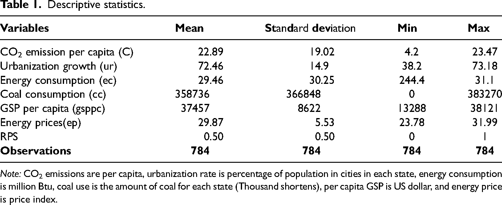
Note: CO₂ emissions are per capita, urbanization rate is percentage of population in cities in each state, energy consumption is million Btu, coal use is the amount of coal for each state (Thousand shortens), per capita GSP is US dollar, and energy price is price index.

Results and discussion

The Hausman test results show that the calculated χ² is 32.86 (Table 2), which denotes that the estimated parameters are biased under the specification of random effects. Based upon the LR tests in Table 2 for nonspatial models, we can conclude that both the state and time period fixed effects should be added to the model. As noted earlier, the Wald tests show that the SDM is the best spatial panel model (Table 2).

Table 2.

Post diagnostic tests.

Tests	Non-spatial and spatial	Joint significant for FE	Spatial specification
Likelihood ratio (LR):	State fixed effect (SFE)	128.35 (0.000)	-
	Time fixed effect (TFE)	42.67 (0.000)	-
	Spatial lag	-	84.92 (0.000)
	Spatial error	-	72.54 (0.000)
Hausman	-	32.86 (0.000)	-
Wald:	Spatial lag	-	70.45 (0.000)
Wald:	Spatial error	-	76.08 (0.000)

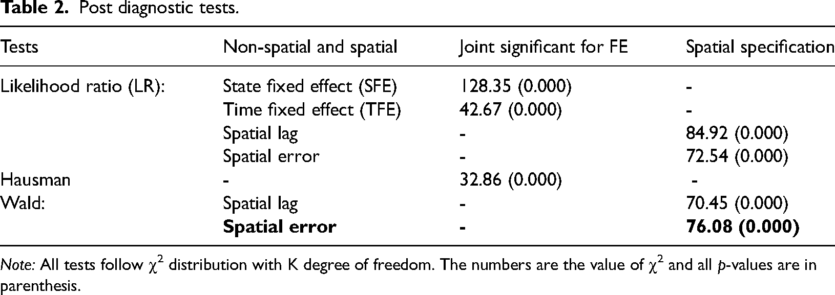
Note: All tests follow χ² distribution with K degree of freedom. The numbers are the value of χ² and all p-values are in parenthesis.

Table 3 shows the results of the SDM. The ρ_sdm coefficient is positive and statistically significant, justifying the use of spatial econometric models by indicating the presence of a spatial autoregressive impact. This coefficient shows that an increase in CO₂ emissions in neighboring states leads to an increase of approximately 0.2 times emissions in adjacent states. This result implies that if spatial dependence is ignored, interpreting estimated impacts with OLS will be incorrect.

Table 3.

Estimation results of non-spatial, panel data models.

Dependent variable: CO₂ emissions per capita	1. 1. (1)	2. 2. (2)	3. 3. (3)	4. 4. (4)
Constant	−5.89** (−1.06)	NA	NA	NA
Urbanization rate (ur)	−0.021** (0.013)	0.023*** (0.004)	0.04 (0.58)	0.59 (0.61)
Energy consumption (ec)	1.039*** (0.03)	0.10 (0.40)	−0.003 (0.056)	0.023 (0.19)
Coal consumption (cc)	1.30*** (0.03)	1.04*** (0.02)	1.07*** (0.07)	1.01*** (0.03)
GSP per capita (gsppc)	−0.05** (0.03)	−0.44*** (0.03)	−0.26*** (0.05)	−0.78*** (0.006)
Energy prices(ep)	−0.34** (0.09)	−0.25*** (0.07)	−0.41** (0.10)	−0.65 (2.94)
RPS	−0.026*** (0.009)	-.017*** (0.007)	−0.15*** (0.004)	−0.31*** (0.001)
LM spatial lag	67.24***	20.17***	12.83***	8.94***
LM spatial error	27.34***	13.69***	7.01***	08***
σ²	0.12	0.03	0.06	0.04
R²	0.58	0.52	0.67	0.36
Observations	784	784	784	784

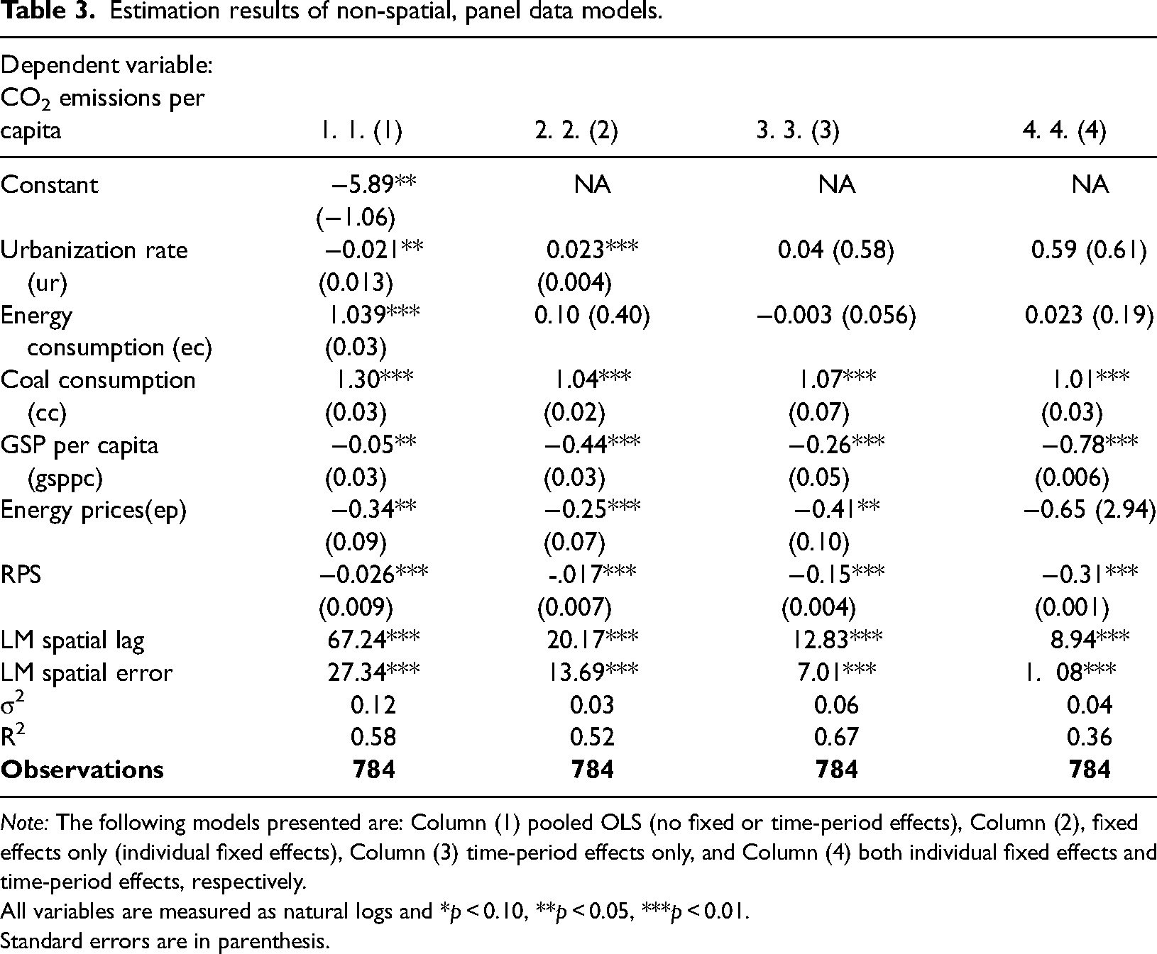
Note: The following models presented are: Column (1) pooled OLS (no fixed or time-period effects), Column (2), fixed effects only (individual fixed effects), Column (3) time-period effects only, and Column (4) both individual fixed effects and time-period effects, respectively.

All variables are measured as natural logs and *p < 0.10, **p < 0.05, ***p < 0.01.

Standard errors are in parenthesis.

Statistically significant and negative direct effects include urbanization rate, energy prices, RPS, and per capita GSP, while energy use and coal consumption have statistically significant positive direct effects (Table 3). These results indicate that increased urbanization, energy prices, and economic growth along with the passage of an RPS will decrease state-level CO₂ emissions, while increasing coal consumption and energy use will lead to increased emissions. Coal consumption dramatically increases CO₂ emissions with a 1% increase leading to an own state increase of 1.31% in emissions and a total effect of more than double at 2.54%. The size of the total effect for coal consumption indicates that encouraging the replacement of coal with renewable or natural gas energy plays a critical role in decreasing CO₂ emissions.

Table 4 reports the estimation results for direct and indirect effects from the SDM model. Among the direct effects, each independent variable has a statistically significant impact at a 1% level, except for coal consumption which is significant at the 5% level. Table 4 illustrates direct and indirect impacts of predictors on CO₂ emissions. Indirect effects are statistically significant apart from per capita GSP. The negative direct effect and positive indirect effect of urbanization rate suggest that growth in urbanization will reduce own state CO₂ emissions while at the same time increasing emissions of neighboring states. These results imply that a 1% increase in urbanization is linked with a 0.3% decrease in own state per capita CO₂ emissions and an 0.012% increase in per capita emissions in neighboring states. The intuition here is that the total effect of urbanization advances reductions in CO₂ emissions so growing cities across the United States has a total effect of decreasing CO₂ emissions.

Table 4.

Estimation results of direct, indirect, and total effect of the SDM.

Dependent variable:CO₂	Direct effect	Indirect effect	Total effect
Urbanization rate (ur)	−0.30*** (0.03)	0.012** (0.005)	−0.288** (0.09)
Energy consumption (ec)	0.53*** (0.05)	0.49*** (0.07)	1.02** (0.15)
Coal consumption (cc)	1.31** (0.60)	1.23** (0.37)	2.54** (1.20)
GSP per capita (gsppc)	−0.57*** (0.10)	−0.74 (1.12)	−1.31*** (0.11)
Energy prices(ep)	−0.28*** (0.047)	−0.46*** (0.020)	−0.74*** (0.08)
RPS	−0.014*** (0.006)	−0.015*** (0.0047)	−0.029*** (0.004)
Observations	784	784	784

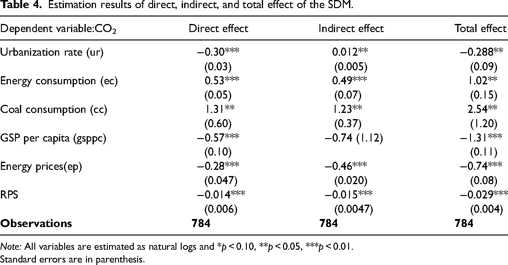
Note: All variables are estimated as natural logs and *p < 0.10, **p < 0.05, ***p < 0.01.

Standard errors are in parenthesis.

Energy and coal consumption have positive direct and indirect effects on CO₂ emissions, implying that an increase in either one leads to emission increases, both own state and neighboring states. In fact, coal and energy consumption as electrical energy in power plants generate CO₂ emissions. The statistically significant effect of per capita GSP is negative within own state emission, but the indirect effect is not statistically significant. This result suggests that if the own state per capita GSP increases, it will lead to own state CO₂ emissions reductions, but not reductions in neighboring states. The estimated coefficients on the GSP are all highly significant and consistent with the inverted U-shaped relationship illustrated by the environmental Kuznets curve (EKC) hypothesis. As shown in Table 3, the negative direct and indirect effects of energy prices suggest that if state-level energy prices increase, this effect will not only decrease in-state CO₂ emissions but also CO₂ emissions from neighboring states by an even larger amount. The estimate shows that energy price linkage to CO₂ emissions is inelastic in the short run. This indicates that the result is consistent with expectations as in the short run consumers do not have the possibility to change their quantity of energy and can only alter the behavior of consumers (Bhattacharyya, 2011). In other words, if one state increases its energy prices then it has a negative, short-run impact on its own CO₂ emissions. In accordance with the law of demand it is expected that all coefficients on the prices are negative (Table 3).

Finally, with negative direct and indirect effects, if an RPS is implemented in one state, it will lead to reductions in own state CO₂ emissions as well as an equally large reduction of emissions in neighboring states. This effect is indicative of interstate electricity transport and renewable energy certificates for electricity generation that can be traded across state lines.

The estimated results for spatial models are reported in Table 5. The results show that at a 1% statistical significance level, CO₂ emissions are a decreasing function of explanatory variables for urbanization rate, energy prices, RPS, and per capita GSP. Table 5 also reveals that at a 1% statistical significance level, CO₂ emissions are increasing functions of energy use and coal consumption. The ρ_sdm coefficient in the SDM model is statistically significant with contiguity-based matrix, justifying the use of spatial econometric models by indicating the presence of a spatial autoregressive impact. Therefore, dynamic spillover long-run linkages between fossil fuel energy use and urbanization are of importance to energy policy makers in the United States. Policy toward lessening coal consumption might have a significant impact on the reduction of CO2 emissions in the states. The implications of this study for policy are as follows. First, U.S. utilities are using more clean energy and substituting natural gas for coal, as this substitution is affected by both efficiency and the price of natural gas. Since the coal industry has been in crisis, it is proper policy to promote exporting coal to other countries might be a solution to overcome the industry's crisis. Second, since there are not statistically significant, long-run impacts from any variables on coal consumption in the post shale gas time period, the expansion of shale gas production has substantially changed the factors that determine coal consumption. On the one hand, this substitution has resulted in important shifts in the U.S. energy market and reducing CO₂ emissions. On the other hand, this substitution implies that another proper policy could be to encourage using coal for other uses (i.e. manufacturing or steel industry).

Table 5.

Estimation results of spatial panel data models

Dependent variable: CO₂ emissions per capita	SAR	SEM	SDM
Urbanization rate (ur)	−0.28***(0.05)	−0.34*** (0.04)	−0.47*** (0.08)
Energy consumption (ec)	2.10*** (0.38)	0.55*** (0.07)	1.32***(0.09)
Coal consumption (cc)	1.56***(0.04)	1.34*** (0.05)	1.40*** (0.05)
GSP per capita (gsppc)	−0.22*** (0.07)	−0.83*** (0.25)	−0.41*** (0.06)
Energy prices(ep)	−0.12*** (0.01)	−0.35***(0.11)	−0.62***(0.03)
RPS	−0.18***(0.007)	0.21***(0.009)	−0.25***(0.005)
Ρ	0.22***(0.02)	NA	0.20***(0.015)
⋋	NA	0.56***(0.04)	NA
w* Urbanization rate (ur)	NA	NA	0.043***(0.004)
w*Energy consumption (ec)	NA	NA	0.55** (0.06)
w* coal consumption (cc)	NA	NA	1.001*** (0.34)
w* GSP per capita (gsppc)	NA	NA	−0.64*** (0.02)
w *Energy prices(ep)	NA	NA	0.52 (0.93)
w *RPS	NA	NA	0.07***(0.005)
σ²	0.07	0.06	0.04
R²	0.72	0.69	0.75
Observations	784	784	784

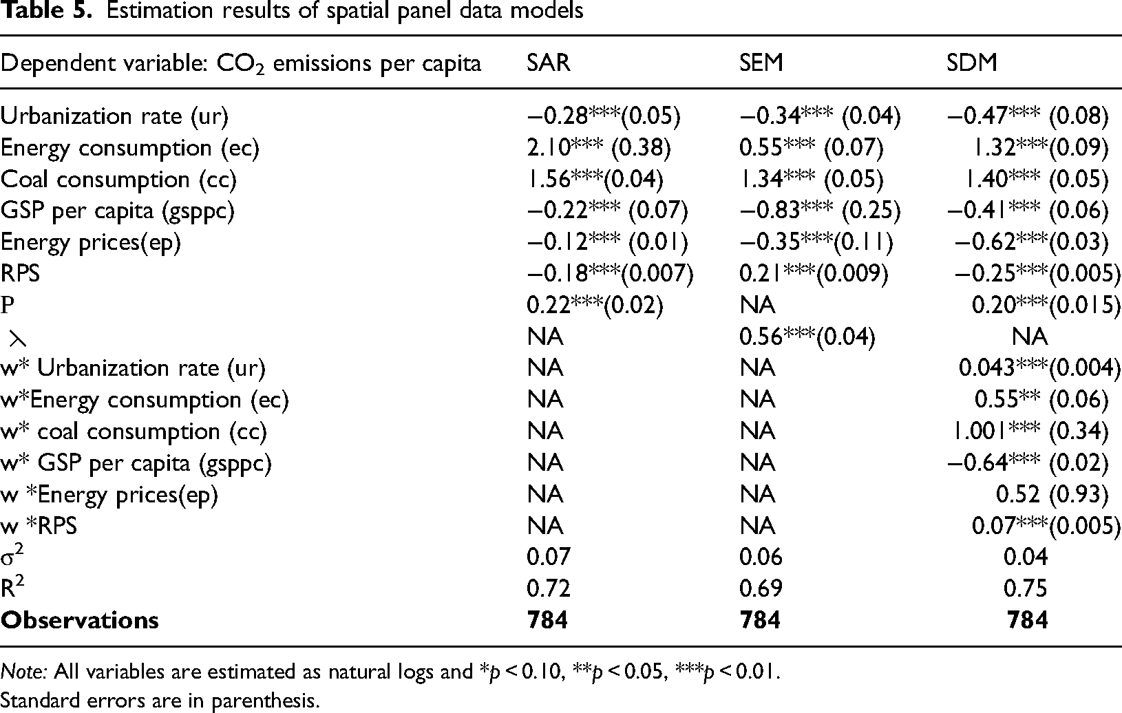
Note: All variables are estimated as natural logs and *p < 0.10, **p < 0.05, ***p < 0.01.

Standard errors are in parenthesis.

These empirical results not only contribute to advancing the current literature but also deserve certain attention from energy policy makers in the U.S. market. Since more than 90% coal have been used in power plants in the United States, as capacities of power plants are decreasing and new capacities are being established to replace them, power firms are promoting to use of more efficient and cost-effective energy sources (i.e. natural gas) to build new power plants over coal-fired plants. Given the coal issue of the energy market in the United States, more study needs to be undertaken to offer a comprehensive resource for policymakers pursuing actual solutions to alleged problems surrounding this industry. Thus, a U.S. state is more likely to adopt a law and or policy if its neighboring states have already done so (Mooney, 2001). In fact, geographical location has been identified as a critical factor of cross-region economic growth due to indicators like the diffusion of technology (Keller, 2004). We could argue that CO₂ emissions may decrease with technological development, then the diffusion of technology would likely enhance conditions of neighboring environment. It is important to develop federal and state policy to manage CO₂ emissions in the cities. Moreover, other policies to decrease CO₂ emissions would promote developing urban areas and implement a renewable energy policy.

Conclusions

The empirical results suggest that urbanization rate, energy prices, RPS, and per-capita GSP are inversely related to CO₂ emissions in their own states. These results imply that increased urban development, economic growth, and the implementation of RPS all reduce CO₂ emissions at the state level. The SDM also shows that while more urbanization reduces the own state CO₂ emissions, it increases CO₂ emissions of neighboring states by about 1/3 amount of the own state reduction. One possible reason for this positive indirect effect of urbanization stems from interstate transportation of goods and services. As urban areas grow, there is increased importation of goods and products from other states, which create energy-related CO₂ emissions from the production and transportation of these goods.

The direct and indirect effect results of the energy use and coal consumption variables imply that higher coal consumption and energy use lead to higher CO₂ emissions not only within a state but also on a regional basis. Hence, reducing fossil fuel use in an economy is an effective choice for decreasing CO₂ emissions. Coal consumption has the highest impact on CO₂ emissions of any variable, which suggests that an appropriate policy for reducing CO₂ emissions is to use more efficient energy sources and renewable energy.

Our results contribute to the literature by quantifying opposite direct and indirect effects of urbanization on state-level CO₂ emissions along with the negative effects of income and RPS on state-level emissions. The income effects provide additional support for the EKC, such that income growth reduces per capita CO₂ emissions (Aldy, 2005; Tawfeeq et al., 2019). For RPS, the indirect effects of CO₂ emission reductions are as large as the own state direct effects, indicating that cross-border impacts are important. This result is important due to the prominence of state and local government actions in climate change mitigation now that the U.S. government has withdrawn from the Paris Climate Accords.

However, this study suffers from several limitations. First, the problem of measurement error of CO₂ emissions that is consistent with the rest of literature since CO₂ emission is based on the measurement of emissions from the burning of fossil fuels and not real ambient CO₂ emissions. Second, there are other factors that contribute to CO₂ emissions that include land use conversions from natural areas or farm to urban which are necessary to create urbanization. These factors are not accounted for in this analysis. Third, the spatial panel data process could suffer from problems of endogeneities within the independent variables and issue of theoretical framework.

The impacts of factors and independent variables from Table 4 are essentially consistent with the previous literature and theoretical expectations offered in literature review and the theoretical model (Newman and Kenworthy, 1999; Cole and Neumayer, 2004; Andrews, 2008; Gonzalez, 2009; Jaforullah and King, 2017). More specifically, our results are in line with the findings of Liddle and Lung (2010), Poumanyvong and Kaneko (2010), Chuai et al. (2012), and Burnett et al. (2013) since they had evidence favorable to the effects of urbanization, GDP, and the energy factors (use, prices, and policies) on CO₂ emissions. However, our study contrasts with some of these studies since our findings show that urbanization has negative direct effect and positive indirect effects on CO₂ emissions at the state level in the United States. Finally, this study only provides a primary interpretation of the effect of urbanization on CO₂ emissions based upon state-level data. Hence, it excludes more explicit factors examining city size, green technologies implemented, substitutions of renewable energy for fossil fuels, and structural changes among various economic sectors in the U.S. urban areas. Future work could be to more directly investigate the roles of economic activities, sectors of economy in urban areas, renewable energy sources, and other excluded factors in explaining the effect of urbanization on environment and economic development. We look forward to future study along with these lines.

Footnotes

Declaration of conflicting interests

The author(s) declared no potential conflicts of interest with respect to the research, authorship, and/or publication of this article.

Funding

The author(s) received no financial support for the research, authorship, and/or publication of this article.

ORCID iD

Mousa Tawfeeq

Notes

References

Adedoyin

Agboola

Ozturk

, et al. (2021) Environmental consequences of economic complexities in the EU amidst a booming tourism industry: Accounting for the role of Brexit and other crisis events. Journal of Cleaner Production 305: 127117.

Aldy

(2005) Environmental Kuznets curve analysis of U.S. state-level carbon dioxide emissions. Journal of Environment & Development 14(2): 48–72.

Andrews

(2008) Greenhouse gas emissions along the rural-urban gradient. Journal of Environmental Planning and Management 51(6): 847–70.

Anselin

(2002) Under the hood issues in the specification and interpretation of spatial regression models. Agricultural Economics 27(3): 247–267.

Anselin

Gallo

Jayet

(2008) Spatial panel econometrics. The Econometrics of Panel Data: Fundamentals and Recent Developments in Theory and Practice: 625–660.

Auffhammer

Carson

(2008) Forecasting the path of China's CO₂ emissions using province-level information. Journal of Environmental Economics and Management 55: 229–247.

Baltagi

Bresson

Pirotte

(2012) Forecasting with spatial panel data. Computational Statistics & Data Analysis 56(11): 3381–3397.

Bekun

(2022) Mitigating emissions in India: accounting for the role of real income, renewable energy consumption and investment in energy. 670216917.

Bhattacharyya

(2011) Energy Economics: Concepts, Issues, Markets, and Governance. London, UK: Springer-Verlag.

10.

Burnett

Bergstrom

Dorfman

(2013) A spatial panel data approach to estimating US state-level energy emissions. Energy Economics 40: 396–404.

11.

Canadell

Le Quéré

Raupach

, et al. (2007) Contributions to accelerating atmospheric CO₂ growth from economic activity, carbon intensity, and efficiency of natural sinks. Proceedings of the National Academy of Sciences 104(47): 18866–18870.

12.

Carson

(2010) The environmental Kuznets curve: Seeking empirical regularity and theoretical structure. Review of Environmental Economics and Policy 4(1): 3–23.

13.

Chuai

Huang

Wang

, et al. (2012) Spatial econometric analysis of carbon emissions from energy consumption in China. Journal of Geographical Sciences 22(4): 630–642.

14.

Cole

Neumayer

(2004) Examining the impact of demographic factors on air pollution. Population and Environment 26(1): 5–21.

15.

Conley

Ligon

(2002) Economic distance and cross-country spillovers. Journal of Economic Growth 7(2): 157–87.

16.

Davis

Peters

Caldeira

(2011) The supply chain of CO2 emissions. Proceedings of the National Academy of Sciences 108(18): 554–559.

17.

Elhorst

(2009) Spatial panel data models. In: Fischer

Getis

(eds) Handbook of Applied Spatial Analysis. Berlin: Springer-Verlag, 377–407.

18.

Elhorst

(2012) Dynamic spatial panels: Models, methods, and inferences. Journal of Geographical Systems 14(1): 5–28.

19.

Elhorst

(2014) Spatial panel data Models. Spatial Econometrics: From Cross-Sectional Data to Spatial Panels: 37–93.

20.

Getis

(2007) Reflections on spatial autocorrelation. Regional Science and Urban Economics 37(4): 491–496.

21.

Gonzalez

(2009) Urban Sprawl, Global Warming, and the Empire of Capital. Albany, NY: State University of New York Press.

22.

Hausman

Taylor

(1981) Panel data and unobservable individual effects. Econometrica: Journal of the Econometric Society: 1377–1398.

23.

International Energy Agency (2020) Available at: https://www.iea.org/reports/globalabc-roadmap-for-buildings-and-construction-2020-2050.

24.

Itkonen

(2012) Problems estimating the carbon Kuznets curve. Energy 39(1): 274–280.

25.

Iwata

Okada

Samreth

(2012) Empirical study on the determinants of CO2 emissions: Evidence from OECD countries. Applied Economics 44(27): 3513–3519.

26.

Jaforullah

King

(2017) The econometric consequences of an energy consumption variable in a model of CO2 emissions. Energy Economics 63: 84–91.

27.

Keller

(2004) International technology diffusion. Journal of Economic Literature 42(3): 752–782.

28.

Kindle

Shawhan

(2011) An empirical test for inter-state carbon-dioxide emissions Leakage resulting from the regional greenhouse gas initiative. Technical Report, Rensselaer Polytechnic Institute.

29.

LeSage

Pace

(2009) Introduction to Spatial Econometrics. Taylor & Francis Group, LLC.

30.

Liddle

Lung

(2010) Age-structure, urbanization, and climate change in developed countries: Revisiting STIRPAT for disaggregated population and consumption-related environmental impacts. Population and Environment 31(5): 317–343.

31.

Martinez-Zarzoso

Maruotti

(2011) The impact of urbanization on CO₂ emissions: Evidence from developing countries. Ecological Economics 70: 1344–1353.

32.

Mooney

(2001) Modeling regional effects on state policy diffusion. Political Research Quarterly 54(1): 103–124.

33.

Mujtaba

Jena

Bekun

, et al. (2022) Symmetric and asymmetric impact of economic growth, capital formation, renewable and non-renewable energy consumption on environment in OECD countries. Renewable and Sustainable Energy Reviews 160: 112300.

34.

Newman

Kenworthy

(1999) Sustainability and Cities: Overcoming Automobile Dependence. Washington, DC: Island Press.

35.

Ongan

Işık

Bulut

, et al. (2022) Retesting the EKC hypothesis through transmission of the ARMEY curve model: An alternative composite model approach with theory and policy implications for NAFTA countries. Environmental Science and Pollution Research: 1–13.

36.

Peters

Minx

Weber

, et al. (2011) Growth in emission transfers via international trade from 1990 to 2008. Proceedings of the National Academy of Sciences of the United States of America 108(8): 903–908.

37.

Poumanyvong

Kaneko

(2010) Does urbanization lead to less energy use and lower CO₂ emissions? A cross-country analysis. Ecological Economics 70(2): 434–444.

38.

Sadorsky

(2014) The effect of urbanization on CO₂ emissions in emerging economies. Energy Economics 41: 147–153.

39.

Shahbaz

Bhattacharya

Ahmed

(2017) CO2 emissions in Australia: Economic and non-economic drivers in the long-run. Applied Economics 49(13): 1273–1286.

40.

Soytas

Sari

Ewing

(2007) Energy consumption, income, and carbon emissions in the United States. Ecological Economics 62: 482–489.

41.

Tawfeeq

Collins

Elbakidze

, et al. (2019) Linking crude oil prices and Middle East stock markets. OPEC Energy Review 43(2): 136–167.

42.

Tawfeeq

Collins

Nowak

(2020) The dynamic response of coal consumption to energy prices and GDP: An ARDL approach to the US. AIMS Energy 8(6): 1156–1172.

43.

U.S. Energy Information Administration (EIA) (2020) Dataset and U.S. Energy Markets. Available at: https://www.eia.gov/.

44.

Wang

Zhou

, et al. (2011) CO2 emissions, energy consumption and economic growth in China: A panel data analysis. Energy Policy 39: 4870–4875.

45.

York

Rosa

Dietz

. (2003) STIRPAT, IPAT and impact: Analytic tools for unpacking the driving forces of environmental impacts. Ecological Economics 46(3): 351–365.

The spillover impacts of urbanization and energy usage on CO 2 emissions: A regional analysis in the United States

Abstract

Keywords

Introduction

Theoretical model

Empirical model

Data description

Results and discussion

Conclusions

Footnotes

Declaration of conflicting interests

Funding

ORCID iD

Notes

References