Flaky cuttings bed distribution model in a shale gas horizontal well based on experiment and numerical simulation

Abstract

During the drilling of shale gas wells, the shape of shale cuttings cut by polycrystalline diamond compact bits has an obvious flaky structure. The accumulation of such flaky cuttings is one of the main reasons for high drilling torque and drag and serious back pressure, which affect the drilling speed of the horizontal section of shale gas wells. Therefore, predicting the thickness of the flaky cuttings bed and restraining it are essential for ensuring safe and efficient drilling of the horizontal section of shale gas wells. However, most of the previous research on migration laws for cuttings were based on spherical particles, which affected the accuracy of cuttings bed thickness prediction. In this study, through visualization experiments combined with computational fluid dynamics numerical simulation, the hole cleaning laws of shale gas wells in the long horizontal section were studied, and a set of cuttings bed thickness prediction models and cuttings bed removal process parameter optimization methods were established. Field application was conducted in the Changning 209H24-1 well in the southern Sichuan Basin, China. The results revealed the following: (1) There are significant differences in the migration laws of flaky cuttings and spherical cuttings in the horizontal section. (2) The fitting accuracy of the established long horizontal fragmentation layer distribution model considering multiple factors and the experimental data is as high as 0.973. (3) Based on this model, the drilling parameters of the Changning 209H24-1 well were optimized, which played a good role in wellbore cleaning and ensured the safe and smooth implementation of the later casing operation.

Introduction

In recent years, because of the increasing demand for oil and natural gas, shale gas, which has the characteristics of being rich in resources, having low carbon impact, and offering environmental protection, has become a clean energy source that has attracted much attention. Because of the low permeability and heterogeneity of shale gas reservoirs, horizontal well technology has become an important technology for shale gas development and increasing production (Chen et al., 2020; Epelle & Gerogiorgis, 2017; Ma et al., 2021). Compared with vertical wells, horizontal wells have higher single well production (Allahvirdizadeh et al., 2016). However, because of gravity, the cuttings in the horizontal section are often deposited in the form of cuttings beds, and the migration of these cuttings can become a problem for horizontal wells. Cuttings migration in the horizontal section of a horizontal well is mainly a solid–liquid two-phase flow of drilling fluid and cuttings particles. Liquid flow characteristics and cuttings characteristics are the two core factors that affect the migration of cuttings. Different process parameters during the construction process, such as annulus size, eccentricity, drilling fluid displacement, drill pipe rotation speed, rheological mode, angle of inclination, and performance of the drilling fluid, mainly affect the flow characteristics of the annulus fluid, while the size, density, and shape of drill cuttings mainly affect its force and movement in the drilling fluid (Cho et al., 2001; Duan et al., 2008; Ford et al., 1990; Gulraiz & Gray, 2021; Han et al., 2010; Huque et al., 2020; Ozbayoglu et al., 2008; Song et al., 2017; Zhang et al., 2015; Zhu et al., 2021).

Since the 1960s, many researchers have conducted considerable research on cuttings migration in horizontal wells, among which a typical model is the stratification model of cuttings migration in a horizontal annulus (Azar & Sanchez, 1997; Cho et al., 2000; Walker & Li, 2000). In the study of cuttings migration in horizontal wells and inclined wells, obvious stratification has been observed in many experiments. Tomren et al. (1986), one of the earliest scholars who studied the migration of cuttings in inclined wells, found that there may be three layers when drilling fluid and cuttings flow in the borehole. Gavignet & Sobey (1989) took the lead in putting forward a two-layer flow model describing liquid flow and particle beds in an inclined well annulus and established a mathematical model of cuttings migration. Doron & Barnea (1993) proposed a more complicated three-layer model, aiming at the situation in which the two-layer model could not meet the prediction at low flow rate. The whole annular flow was divided into three parts: the lowest fixed cuttings bed area, the middle moving cuttings bed with mixed solid–liquid flow, and the upper heterogeneous suspended flow area. To improve the evaluation and description of hole cleaning in highly deviated wells, Nguyen & Rahman (1998) put forward a new three-layer model based on the early three-layer model, which allowed for a better understanding of the theory and mechanism of cuttings migration. Guo et al. (2010) considered the mechanism of cuttings suspension, rolling and sliding, the relative velocity of solid and liquid in the suspension layer, and the influence of drill pipe rotation and proposed a three-layer unsteady cuttings migration model. By solving these models, the general concentration distribution and average velocity distribution of each phase can be determined. However, the calculation process is complicated because there are many equations needed for closure.

Other scholars have studied the overall migration velocity of cuttings from a macro perspective. Usually, based on a large number of experiments or field data analysis, relevant empirical formulas are established, the annular cuttings are regarded as a whole, the annular transmission speed of cuttings is defined as a whole, and the influence of relevant parameters is analyzed. Ozbayoglu et al. (2008) also put forward an empirical formula of cuttings bed thickness and a formula for the friction pressure drop considering the influence of drill string rotation for the angle of inclination in the range of 60°–90° by using a dimensional analysis method combined with experimental data. The predicted results of these two formulas are in good agreement with the experimental results. Shadizadeh & Zoveidavianpoor (2012) built a model based on the concept of the minimum transport velocity of cuttings and performed an experimental study on the influence of drilling fluid rheological model, particle size, drilling fluid displacement, annulus size, and other factors on the migration velocity of cuttings. Sorgun (2013) used experimental data to give an empirical formula for estimating the thickness of the cuttings bed in horizontal wells and inclined wells for water and non-Newtonian fluids, respectively, and discussed the migration mechanism of cuttings in the annulus when the drill pipe rotates. Because of the different experimental conditions and the different influencing factors, the experimental data have certain limitations, and each model has its scope of application. So far, there is no universal model.

Because the theoretical model and empirical model ignore many influencing factors, and the actual interaction between particles and between the solid and liquid phases is so complicated, there is still a significant gap between the models and reality. By the 21st century, with the development of computational fluid dynamics (CFD) and the maturity of CFD and discrete element method simulation software, researchers tended to study the migration of cuttings by combining numerical simulation with theory and experiment. Akhshik et al. (2015) used the combination of CFD and the discrete element method to simulate the annulus transport. By considering the collision between drilling tools and the borehole wall, a CFD–discrete element method model was established. The results show that, under the conditions of medium and high drilling fluid displacement and low rotation speed, the rotation of drilling tools leads to the cuttings particles being unevenly distributed in the annulus, and the cuttings concentration in the annulus is significantly reduced. When the rotation speed is high and the displacement is low, the drilling tool rotation has no obvious effect on cuttings removal. Ulker & Sorgun (2016) used K-nearest neighbor, support vector regression, linear regression, and artificial neural network models to calculate the thickness of the cuttings bed in the annulus when the drilling tool stops and rotates. Through the analysis of >300 data sets, the thickness of the cuttings bed was found to be in good agreement with the experimental data. Compared with root mean square error, average absolute error, and average absolute percentage error values, the performance of the artificial neural network model was slightly better than that of the other models. However, the modeling speed of the K-nearest neighbor model is much faster than that of other computational intelligence technologies. Naderi & Khamehchi (2018) studied the interaction between various factors in cuttings migration. Both CFD and design of experiments were used to study the influence of different process parameters on the migration efficiency of cuttings. The results showed that the displacement of drilling fluid, rotation speed of drilling tools, and migration speed of cuttings all play a major role in determining the migration efficiency of cuttings.

Through the analysis of the cuttings returning from the site, it is found that the shape of shale cuttings cut by a polycrystalline diamond compact bit has an obvious flaky structure, whereas previous research on the migration law of cuttings in horizontal wells mainly regarded the cuttings particles as spherical and the matching degree with the actual shale cuttings was not high. Therefore, in this study, flaky cuttings are selected as the object to study the migration mechanism of a flaky cuttings bed in a long horizontal section of a shale gas well, and the migration law and related influencing factors of shale cuttings in the horizontal section are studied and analyzed. In the past, scholars have used critical flow rate, minimum flow rate, critical transport fluid velocity, critical flow velocity, minimum transport velocity, critical resuspension velocity, and other critical velocities to study hole cleaning in horizontal and inclined wells (Chen et al., 2014; Duan et al., 2009; Huo et al., 2017; Mohammadsalehi & Malekzadeh, 2011). However, it cannot predict the cuttings bed height when the drilling fluid circulation velocity is less than the critical velocity. When the annular fluid velocity exceeds the critical velocity, the cuttings on the bed are forced into instability and are transported onward to the wellhead. Therefore, the thickness of cuttings bed is studied to evaluate hole cleaning, and a suitable model is established to predict the thickness distribution of the cuttings bed in the entire well section. In the past, the size of the experimental devices established by most scholars was scaled down in proportion, precluding an accurate representation of the migration process of cuttings (Kamyab & Rasouli, 2016; Qu et al., 2021; Sorgun et al., 2011). Therefore, in this study, an experimental device with the same size as the horizontal section of a shale gas well is developed, and the experiment replicates as close as possible the real cuttings migration process. The CFD model was verified by using the experimental results, and the influence of different factors on the thickness of the cuttings bed was further studied on the basis of this model.

This study presents a cuttings bed thickness distribution model considering the rate of penetration (ROP), eccentricity, drill pipe rotation speed, drilling fluid apparent viscosity, drilling fluid displacement, drilling fluid density, well inclination angle, and cuttings shape. The model can be used as a practical reference for the prediction of hole cleaning conditions in horizontal and deviated wells. Predicting the thickness of the cuttings bed provides important practical guidance for the removal of cuttings in the horizontal section of shale gas wells, improving the hole cleaning effect, and guaranteeing safe and efficient construction.

Methodology

Visual experiment

Experimental setup and procedure

Visual methods are suitable for qualitative research and have been increasingly applied in various fields (Pain, 2018). In this study, a large-scale visual experimental device for cuttings migration in horizontal wells was designed and built. The size of the device was developed according to the wellbore structure of the long horizontal section of shale gas wells. The device consists of a drilling fluid system, a cuttings feeding system, a wellbore module, a drill pipe rotation and eccentricity system, a control and data acquisition system, and a cuttings separation system. A schematic diagram and a photograph of the experimental setup are shown in Figures 1 and 2, respectively.

Figure 1.

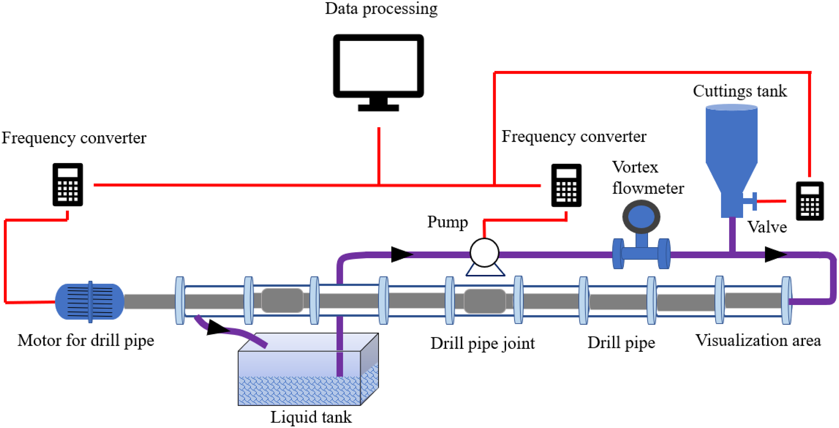
Schematic of the experimental setup.

Figure 2.

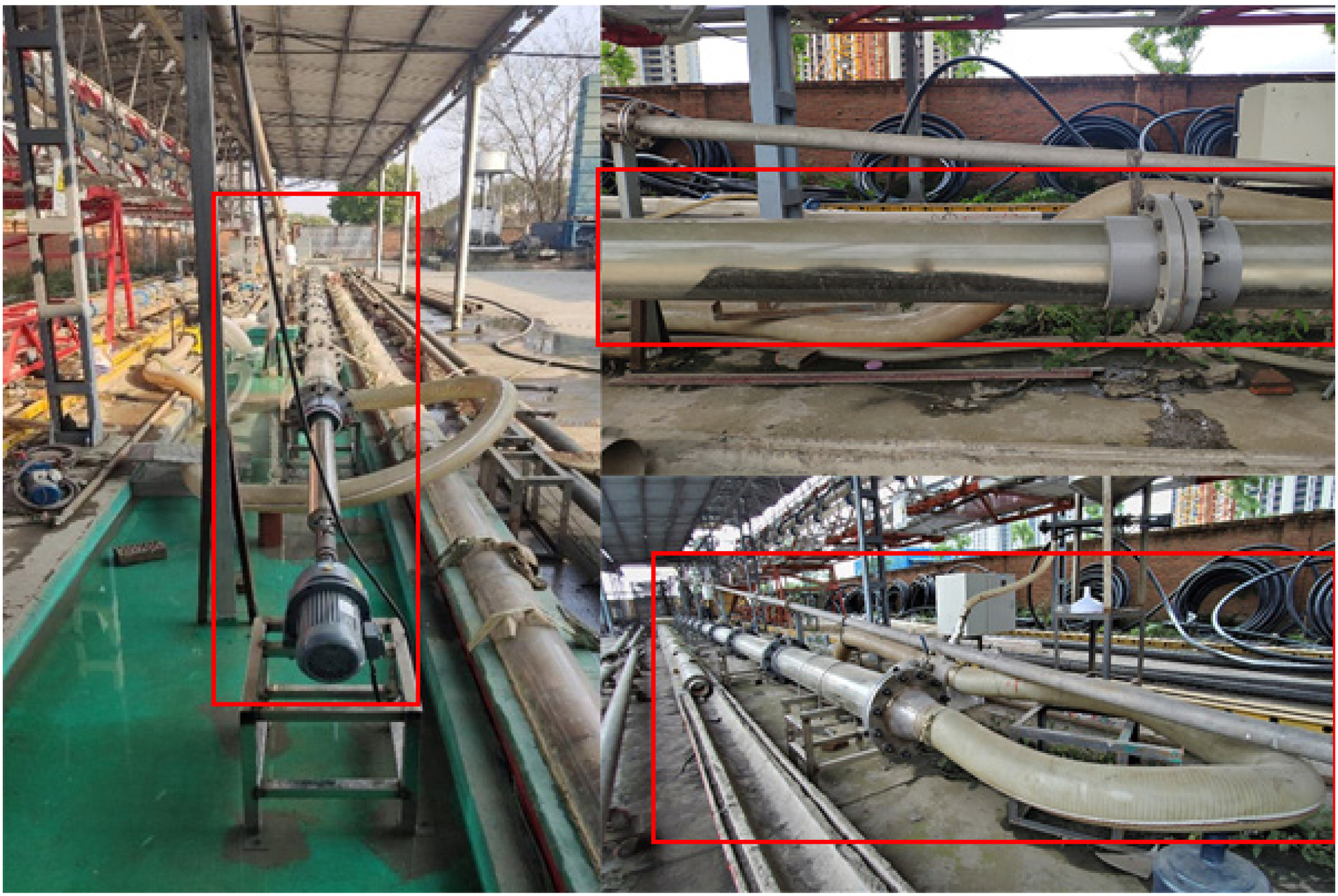
Flow loop unit used for cuttings transport experiments.

The wellbore module comprises a smooth plexiglass tube with an inner diameter of 220 mm and a length of 20.8 m; the wellbore module is placed horizontally. The drill pipe rotation system consists of a drill pipe with a diameter of 127 mm, a drill pipe joint with a diameter of 170 mm, and a motor. The drill pipe can be concentric and eccentric relative to the wellbore. The equipment manufacturers reported that the maximum uncertainties for the liquid flowmeter, eccentricity, and ROP were ± 2%, ± 3%, and ± 0.5%, respectively.

The dimensionless eccentricity of the pipe (e) is shown in Figure 3; eccentricity is defined as follows:

$$e={\displaystyle \frac{2\delta }{D_2\text{-}{D}_1},}$$

(1)

where $\delta$ (mm) is the offset from the center and D₁ (mm) and D₂ (mm) are the drill pipe diameter and borehole diameter, respectively.

Figure 3.

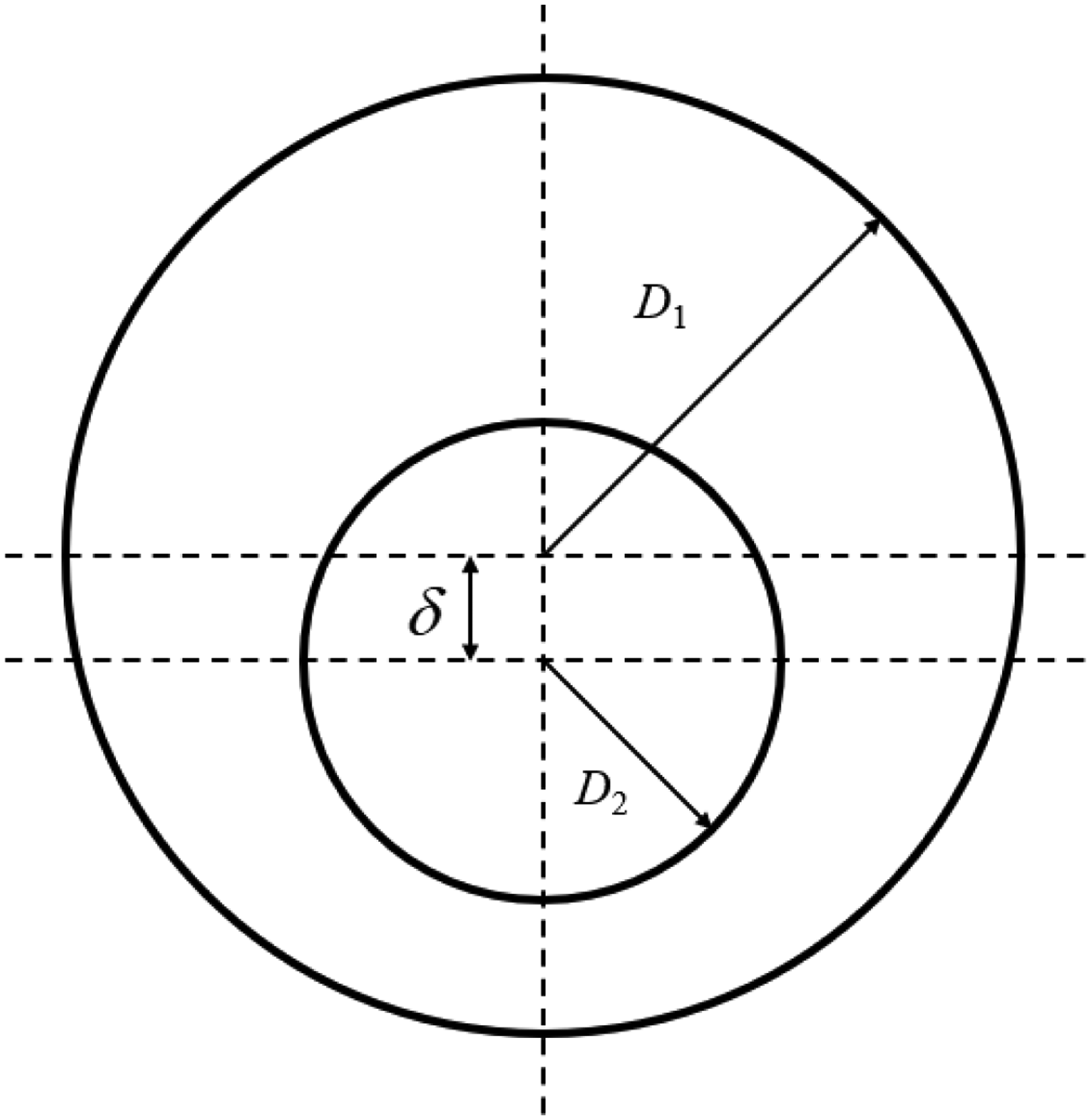
Schematic diagram of eccentricity.

Test particles and drilling fluids

In the experiment, flaky shale pieces (2700 kg/m³) with an equivalent diameter of 2.3 mm and length, width, and height of 4, 2, and 1 mm, respectively, and spherical solid glass balls (2500 kg/m³) with an equivalent diameter of 2.5 mm were used. Two different types of liquids were used in the experiment: (1) clear water and (2) a simulated drilling fluid (made by adding the tackifier carboxyl methyl cellulose and the weighting agent sodium formate to clear water). Carboxyl methyl cellulose does not change the color of the fluid, allowing direct observation of experimental phenomena. The laboratory experiment results showed that the rheological model of the second drilling fluid is the Bingham model. The rheological equation fitted by the experimental data is shown in Eq. (2):

$$\tau =0.1+0.0029\gamma ,$$

(2)

where τ (Pa) is the shear stress and γ (s⁻¹) is the shear rate.

Experimental procedure

Owing to the limitation of the experimental device, it is impossible to achieve a continuous and stable cuttings bed; therefore, in the experiment, we adopted a fixed cuttings quality and took the cuttings removal time as the dependent variable. The experimental procedure was as follows: Store enough test liquid in the liquid tank in advance. Inject 8 kg of cuttings particles into the cuttings tank. Adjust the position of the drill pipe to achieve a predetermined eccentricity. Adjust the frequency converter to cause the drill pipe to rotate at a predetermined speed. Start the drilling fluid pump, and continuously provide a certain flow of drilling fluid to the simulated wellbore through the drilling fluid pump. Turn on the cuttings feeding device, and force the simulated cuttings into the simulated wellbore with the circulation of the drilling fluid. When all the cuttings enter the simulated wellbore, close the feeding device of the cuttings tank. The mixture of cuttings and drilling fluid flowing out of the wellbore passes through the cuttings separation system, the cuttings particles are separated, and the drilling fluid returns to the liquid tank. Record the experimental phenomenon with a camera, and record the time with a stopwatch from when the cuttings enter the simulated wellbore to the time at which the cuttings are completely removed.

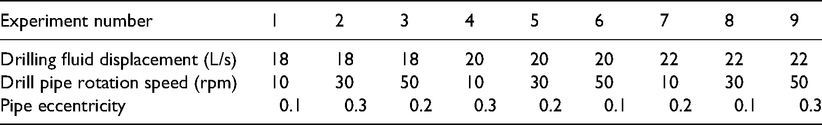
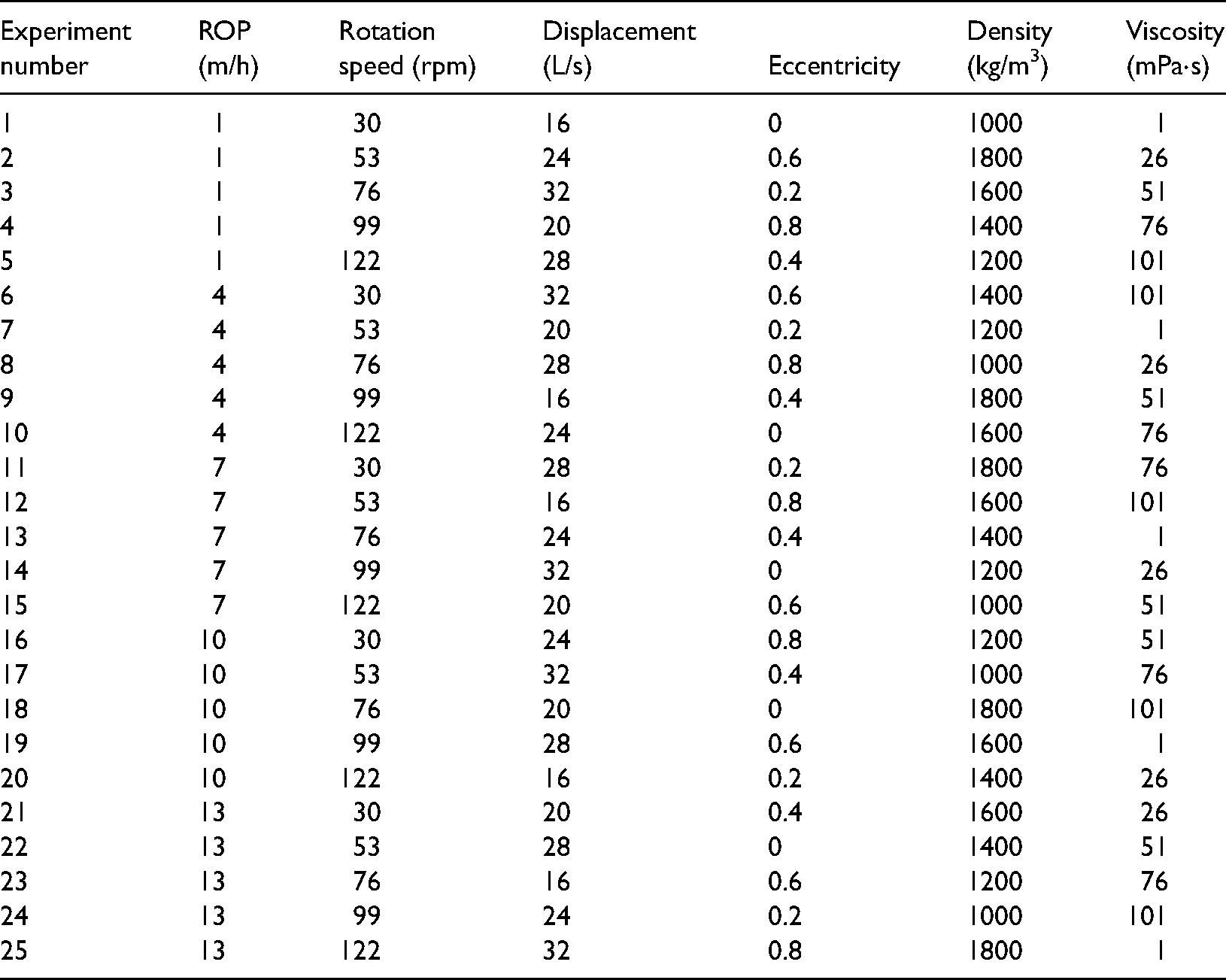
In the experiment, the range of drilling fluid displacement was set to 18–26 L/s, the range of drill pipe eccentricity was 0–0.3, and the range of drill pipe rotation speed was 0–50 rpm, all of which were controlled by corresponding frequency converters. Two experimental methods—a single experiment and an orthogonal experiment—were adopted. The experimental scheme of the orthogonal experiment is presented in Table 1.

Table 1.

Orthogonal experimental scheme.

Experiment number	1	2	3	4	5	6	7	8	9
Drilling fluid displacement (L/s)	18	18	18	20	20	20	22	22	22
Drill pipe rotation speed (rpm)	10	30	50	10	30	50	10	30	50
Pipe eccentricity	0.1	0.3	0.2	0.3	0.2	0.1	0.2	0.1	0.3

Numerical modeling

Although a qualitative law of cuttings migration can be obtained by visual experiments, such experiments cannot be used to evaluate hole cleaning in the long horizontal section of shale gas wells. Because the parameters that can be set in the experiment are limited, and a stable cuttings bed cannot be formed, a numerical simulation was used to expand the research.

Governing equations

In the study of cuttings migration, numerous scholars have used the Euler–Euler model and assumed that the cuttings are spherical particles (Amanna & Khorsand Movaghar, 2016; Awad et al., 2021; Pang et al., 2019). Some scholars have also used the Euler–Lagrange model, assuming that the cuttings are ellipsoid and flake particles (Akhshik et al., 2015; Celigueta et al., 2016). Almohammed et al. (2014) used Euler–Euler and Euler–Lagrange models to compare fluidized beds. Both models can get corresponding results, but the two models have their own advantages and disadvantages. The Euler–Lagrange multiphase flow model is used in this study. In this method, the main phase (drilling fluid) is regarded as the continuous phase, and the sparse phase (cuttings particles) is regarded as the discrete phase. The Navier–Stokes equation is used for the direct solution of the continuous phase. In the discrete phase, the Lagrange method is used for particle tracking by calculating the movement of a large number of particles in the flow field, following the exchange of momentum, mass, and energy between discrete and fluid phases.

Liquid phase

The mass conservation equation can be expressed as

$${\displaystyle \frac{\mathrm{\partial }}{\mathrm{\partial }t}(\alpha {\rho }_f)+\mathrm{\nabla }\cdot (\alpha {\rho }_{\mathrm{f}}\overrightarrow{{\nu }_{\mathrm{f}}})=0,}$$

(3)

where α (%) is the volume fraction of the liquid phase, ${\rho }_{\mathrm{f}}$ (kg/m³) is the liquid density, and $\overrightarrow{{\nu }_{\mathrm{f}}}$ (m²/s) is the liquid velocity.

The momentum conservation equation can be expressed as

$${\displaystyle \frac{\mathrm{\partial }}{\mathrm{\partial }t}(\alpha {\rho }_{\mathrm{f}}\overrightarrow{{\nu }_{\mathrm{f}}})+\mathrm{\nabla }\cdot (\alpha {\rho }_{\mathrm{f}}\overrightarrow{{\nu }_{\mathrm{f}}}\overrightarrow{{\nu }_{\mathrm{f}}})=-\alpha \mathrm{\Delta }p+\mathrm{\nabla }\cdot \overline{\overline{\tau }}+\alpha {\rho }_{\mathrm{f}}\overrightarrow{g}+\sum K_{SL}\mathrm{\Delta }\overrightarrow{\nu }+(\overrightarrow{F_{\mathrm{f}}}+\overrightarrow{F_{lift,f}}+\overrightarrow{F_{vm,f}}),}$$

(4)

where p (Pa) and $\overline{\overline{\tau }}$ (Pa) are the fluid pressure and the stress–strain tensor, respectively, $\overrightarrow{g}$ (m/s²) is the acceleration of gravity, K_SL (dimensionless) is the momentum exchange coefficient between the drilling fluid and cuttings, $\overrightarrow{F_f}$ (N) is the liquid volume force, $\overrightarrow{F_{lift,f}}$ (N) is the liquid lift, and $\overrightarrow{F_{vm,f}}$ (N) is the virtual mass force of the liquid.

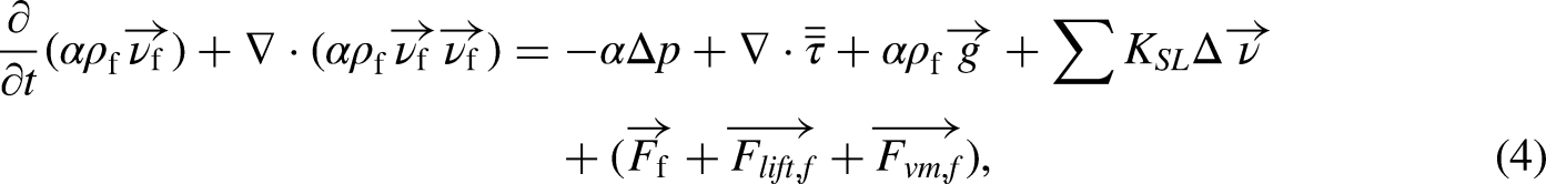
The shear-stress transport model is used in the turbulence model. It is a hybrid model widely used in engineering, and its formulas can be expressed as

$${\displaystyle \frac{\mathrm{\partial }}{\mathrm{\partial }t}(\rho k)+{\displaystyle \frac{\mathrm{\partial }}{\mathrm{\partial }{x}_i}(\rho k{\nu }_i)={\displaystyle \frac{\mathrm{\partial }}{\mathrm{\partial }{x}_j}\left({\mathrm{\Gamma }}_k{\displaystyle \frac{\mathrm{\partial }k}{\mathrm{\partial }{x}_j}}\right)+{\tilde{G}}_k-Y_k,}}}$$

(5)

$${\displaystyle \frac{\mathrm{\partial }}{\mathrm{\partial }t}(\rho \omega )+{\displaystyle \frac{\mathrm{\partial }}{\mathrm{\partial }{x}_j}(\rho \omega u_j)={\displaystyle \frac{\mathrm{\partial }}{\mathrm{\partial }{x}_j}\left({\mathrm{\Gamma }}_{\omega }{\displaystyle \frac{\mathrm{\partial }\omega }{\mathrm{\partial }{x}_j}}\right)+{\tilde{G}}_{\omega }-Y_{\omega }-D_{\omega },}}}$$

(6)

where ${\tilde{G}}_k$ (kg⋅m⁻¹⋅s⁻³) and ${\tilde{G}}_{\omega }$ (kg⋅m⁻¹⋅s⁻³) are the turbulence kinetic energy generated by the average velocity gradient of the kth phase and the ωth phase, respectively; ${\mathrm{\Gamma }}_k$ and ${\mathrm{\Gamma }}_{\omega }$ (dimensionless) are the effective diffusivities of k and ω, respectively; $Y_k$ (kg⋅m⁻¹⋅s⁻³) and $Y_{\omega }$ (kg⋅m⁻¹⋅s⁻³) are the k and ω dissipation caused by turbulence, respectively; and $D_{\omega }$ (kg⋅m⁻¹⋅s⁻³) is the cross-diffusion phase.

1. Solid phase

In FLUENT, the motion trajectory of particles is predicted by considering the force of particles in the Lagrange coordinate system. According to the force acting on particles, the motion equation of particles in the Lagrange coordinate system can be expressed as follows:

$${\displaystyle \frac{d\overrightarrow{{\nu }_p}}{dt}={\displaystyle \frac{\overrightarrow{{\nu }_f}-\overrightarrow{{\nu }_p}}{{\tau }_r}+{\displaystyle \frac{\overrightarrow{g}({\rho }_p-{\rho }_f)}{{\rho }_p}+\overrightarrow{F},}}}$$

(7)

where

$${\tau }_r={\displaystyle \frac{{\rho }_p{d}_p^2}{18\mu }{\displaystyle \frac{24}{C_d\mathrm{Re}},}}$$

(8)

$$\mathrm{Re}={\displaystyle \frac{{\rho }_f{d}_p|\overrightarrow{{\nu }_p}-\overrightarrow{{\nu }_f}|}{\mu },}$$

(9)

$(\overrightarrow{{\nu }_f}\text{-}\overrightarrow{{\nu }_p)}/{\tau }_r$ (N) is the drag force per unit particle mass, ${\tau }_r$ (s) is the relaxation time of particles, $\overrightarrow{{\nu }_p}$ (m/s) is the particle velocity, $\overrightarrow{F}$ (N) is the additional force per unit particle mass; μ (Pa⋅s) is the molecular viscosity of the liquid, ${\rho }_p$ (kg/m³) is the particle density, d_p (m) is the particle diameter, C_d (dimensionless) is the drag coefficient, and Re (dimensionless) is the relative Reynolds number.

• 2) Drag force model

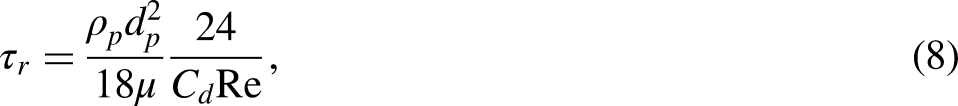
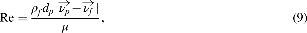
In FLUENT, the drag force coefficient is used to describe the effect of the drag force on particles. According to different particle shapes, drag force coefficient models can be divided into two types: spherical drag force models and nonspherical drag force models. In this study, cuttings are considered as flake cuttings, whose shape is nonspherical, and the spherical coefficient is defined as the ratio of the surface of nonspherical objects to the surface of a sphere of the same volume. The nonspherical drag force model proposed by Haider & Levenspiel (1989) is as follows:

$$C_{\mathrm{d}}={\displaystyle \frac{24}{{\mathrm{Re}}_{\mathrm{sph}}}(1+b_1{\mathrm{Re}}_{\mathrm{sph}}^{b_2})+{\displaystyle \frac{b_3{\mathrm{Re}}_{\mathrm{sph}}}{b_4{\mathrm{Re}}_{\mathrm{sph}}},}}$$

(10)

where

$$b_1=\exp (2.3288-6.4581\varphi +2.4486{\varphi }^2),$$

(11)

$$b_2=\exp (0.0964+0.5565\varphi ),$$

(12)

$$b_3=\exp (4.905-13.8944\varphi +18.4222{\varphi }^2-10.2599{\varphi }^3),$$

(13)

$$b_4=\exp (1.4681+12.2584\varphi -20.7322{\varphi }^2+15.8855{\varphi }^3),$$

(14)

and Re_sph (dimensionless) is the relative Reynolds number of particles with the same volume as the sphere.

• 3) Liquid–solid bidirectional coupling

When the particle trajectory is calculated, the influence of the fluid on the particle and the influence of the particle movement on the fluid are calculated in the whole process. The principle of bidirectional coupling implementation entails solving the governing equations of the continuous phase and the particles alternately until the solutions of both no longer change. In this study, only momentum exchange between liquid and solid phases is addressed.

In a single time step, the momentum exchange between the continuous phase and the discrete phase in a control volume is equal to the change in momentum of the particle:

$$F=\sum \left[{\displaystyle \frac{18\mu C_d\mathrm{Re}}{24{\rho }_p{d}_p^2}({\nu }_p-{\nu }_f)+F_{other}}\right]{\stackrel{\cdot }{m}}_p\mathrm{\Delta }t,$$

(15)

where ${\stackrel{\cdot }{m}}_p$ (kg/s) is the particle mass flow, Δt (s) is the time step, and F_other (N) is other interaction forces.

• 4) Dense discrete phase model

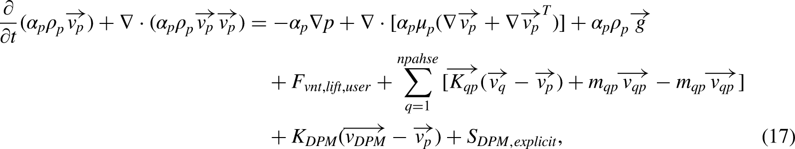
The dense discrete phase model overcomes the limitation of discrete phase volume fraction based on the discrete phase model (DPM). For the dense discrete phase of a single phase P, its continuity equation and momentum conservation equation can be expressed as follows:

$${\displaystyle \frac{\mathrm{\partial }}{\mathrm{\partial }t}({\alpha }_p{\rho }_p)+\mathrm{\nabla }\cdot ({\alpha }_p{\rho }_p\overrightarrow{v_p})=\sum _{q=1}^{npahse}\left({\stackrel{\cdot }{m}}_{qp}-{\stackrel{\cdot }{m}}_{pq}\right),}$$

(16)

$$\begin{array}{rl}{\displaystyle \frac{\mathrm{\partial }}{\mathrm{\partial }t}({\alpha }_p{\rho }_p\overrightarrow{v_p})+\mathrm{\nabla }\cdot ({\alpha }_p{\rho }_p\overrightarrow{v_p}\overrightarrow{v_p})}& =-{\alpha }_p\mathrm{\nabla }p+\mathrm{\nabla }\cdot [{\alpha }_p{\mu }_p(\mathrm{\nabla }\overrightarrow{v_p}+\mathrm{\nabla }{\overrightarrow{v_p}}^T)]+{\alpha }_p{\rho }_p\overrightarrow{g}\\ & +F_{vnt,lift,user}+\sum _{q=1}^{npahse}[\overrightarrow{K_{qp}}(\overrightarrow{v_q}-\overrightarrow{v_p})+m_{qp}\overrightarrow{v_{qp}}-m_{qp}\overrightarrow{v_{qp}}]\\ & +K_{DPM}(\overrightarrow{v_{DPM}}-\overrightarrow{v_p})+S_{DPM,explicit},\end{array}$$

(17)

where K_DPM (dimensionless) represents the interphase momentum exchange coefficient calculated for the average value of the solid volume fraction in the numerical cell and S_DPM,explicit (dimensionless) is the source term related to the particle equation of motion.

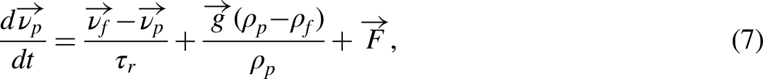
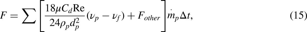
For particles, the following force balance equation is satisfied:

$${\displaystyle \frac{d{v}_p}{dt}=F_D(v_f-v_p)+{\displaystyle \frac{g({\rho }_p-\rho )}{{\rho }_p}+F_{interaction},}}$$

(18)

where $F_D(v_f-v_p)$ (N⋅m/s²) represents the acceleration from the drag force, $\frac{g({\rho }_p-\rho )}{{\rho }_p}$ (m/s²) is the gravitational acceleration, and F_interaction (N) is the additional acceleration resulting from interparticle interactions.

F_interaction is determined as follows:

$$F_{interaction}=-{\displaystyle \frac{1}{{\rho }_p}\mathrm{\nabla }\cdot \overline{{\tau }_s},}$$

(19)

where ${\tau }_s$ (Pa) is the shear stress of the sth particle phase. It can be calculated by using the kinetic theory of particle flow.

Geometric condition

A three-dimensional finite element model of a concentric eccentric drilling annulus was developed, as shown in Figure 4.

Figure 4.

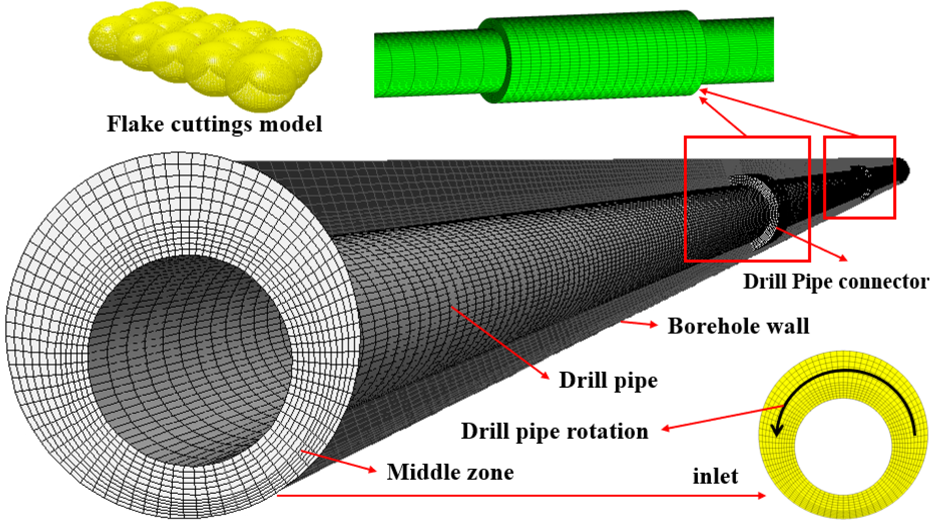
Geometric model and mesh division.

The numerical size of the model is consistent with the experimental device. In the long horizontal section, the drill pipe tends to be eccentric because of the influence of gravity. By defining the distance between the origin of the drill pipe and the center of the borehole wall as eccentricity, an eccentric annulus can be manufactured in simulation. In this study, concentricity (e  =  0) and four eccentricities (e  =  0.2, 0.4, 0.6, and 0.8) were considered.

In the DPM, the concept of particle sphericity is used to represent the shape of irregular cuttings under different aspect ratios. According to the size of cuttings particles tested in this study, the shape coefficient of flaky cuttings particles was set as 0.69. Flaky cuttings particles were randomly injected into the wellbore from the normal direction of the inlet section, and the injection mass flow rate corresponds to the penetration rate.

The dimensionless particle shape factor φ is defined as follows:

$$\varphi ={\displaystyle \frac{s}{S},}$$

(20)

where s (m²) is the surface area of a sphere with the same volume as the particle and S (m²) is the actual surface area of the particle.

Gridding

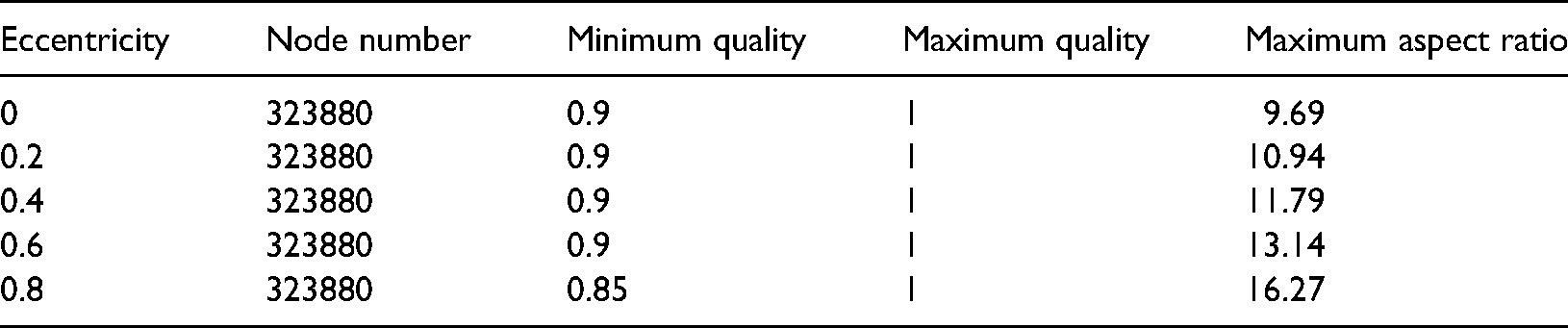
To ensure calculation efficiency and convergence accuracy, the three-dimensional finite element model of the wellbore was discretized into a structured hexahedral mesh. The mesh of the drill pipe joint and the liquid inlet and outlet was refined to improve the quality. The finite element mesh model of cuttings migration in horizontal wells studied is given in Table 2.

Table 2.

Finite element modeling grid parameters.

Eccentricity	Node number	Minimum quality	Maximum quality	Maximum aspect ratio
0	323880	0.9	1	9.69
0.2	323880	0.9	1	10.94
0.4	323880	0.9	1	11.79
0.6	323880	0.9	1	13.14
0.8	323880	0.85	1	16.27

Boundary and initial conditions

The following FLUENT boundary conditions are set:

Mass flow inlet, where the mass flow rate of the drilling fluid into the annulus is described;

Pressure outlet, where the drilling fluid is discharged from the annulus at zero gauge pressure;

Inner wall, which indicates the outer wall surface of the drill pipe; when the drill pipe rotates, this wall surface rotates counterclockwise;

Outer wall, which represents the wellbore wall.

To realize the influence of drill pipe rotation on the liquid–solid mixture, the embedded sliding grid method was adopted. The annular flow zone and the wellbore wall are stationary, and the grid of the drill pipe wall rotates around the axis of the wellbore to provide drill pipe rotation.

Experimental scheme

To study the change of key parameters, the thickness of the cuttings bed was used to evaluate hole cleaning, and the influencing factors of cuttings bed thickness were studied by numerical simulation. According to the technological parameters of shale gas wells, the orthogonal experimental scheme given in Table 3 was designed.

Table 3.

Orthogonal experiment of the simulation design.

Experiment number	ROP (m/h)	Rotation speed (rpm)	Displacement (L/s)	Eccentricity	Density (kg/m3)	Viscosity (mPa⋅s)
1	1	30	16	0	1000	1
2	1	53	24	0.6	1800	26
3	1	76	32	0.2	1600	51
4	1	99	20	0.8	1400	76
5	1	122	28	0.4	1200	101
6	4	30	32	0.6	1400	101
7	4	53	20	0.2	1200	1
8	4	76	28	0.8	1000	26
9	4	99	16	0.4	1800	51
10	4	122	24	0	1600	76
11	7	30	28	0.2	1800	76
12	7	53	16	0.8	1600	101
13	7	76	24	0.4	1400	1
14	7	99	32	0	1200	26
15	7	122	20	0.6	1000	51
16	10	30	24	0.8	1200	51
17	10	53	32	0.4	1000	76
18	10	76	20	0	1800	101
19	10	99	28	0.6	1600	1
20	10	122	16	0.2	1400	26
21	13	30	20	0.4	1600	26
22	13	53	28	0	1400	51
23	13	76	16	0.6	1200	76
24	13	99	24	0.2	1000	101
25	13	122	32	0.8	1800	1

Numerical solution process

The solution to the dense DPM of FLUENT proceeds as follows: (a) Before introducing the particle discrete phase, solve for the fluid flow field. (b) Calculate the phase injection trajectory of each particle. (c) Determine the previously calculated interface momentum exchange, which is used to recalculate the flow field. (d) Recalculate particle trajectories according to the modified flow field. (e) Repeat steps (c) and (d) until a convergent solution is obtained.

Velocity and pressure were coupled using the SIMPLE algorithm, and gradient evaluation was performed using a least-squares element-based method. The momentum equation and the volume fraction equation were solved in the second-order upwind and QUICK formats, respectively. The default automatic high-echelon tracking scheme was used to solve the particle motion equation with a precision tolerance of 10⁻⁵. The bidirectional coupling method was used for testing, and the convergence criterion was determined when the residual was <10⁻⁵.

Experimental results and discussion

Experimental phenomena

Figure 5 shows the experimental phenomena, mainly focusing on three areas: the horizontal annulus, the drill pipe joint, and the rear end joint. Because of the existence of drill pipe joints, the migration process of cuttings bed is not a constant-speed process. The migration of cuttings in the annulus between drill pipe joints is in an accelerated state, and the cuttings bed has a high height, so the migration is fastest when the cuttings pass through the drill pipe joints, while at the back end of the drill pipe joints, accumulation and stagnation occur. Increasing the rotation speed of drill pipes is helpful to remove cuttings at the back end of the joints. Compared with flaky cuttings, spherical cuttings have higher height and a faster speed during migration, as shown in Figures 5(a) and 5(c). For the simulated drilling fluid, more cuttings are found to be suspended in the annulus, as shown in Figure 5(b).

Figure 5.

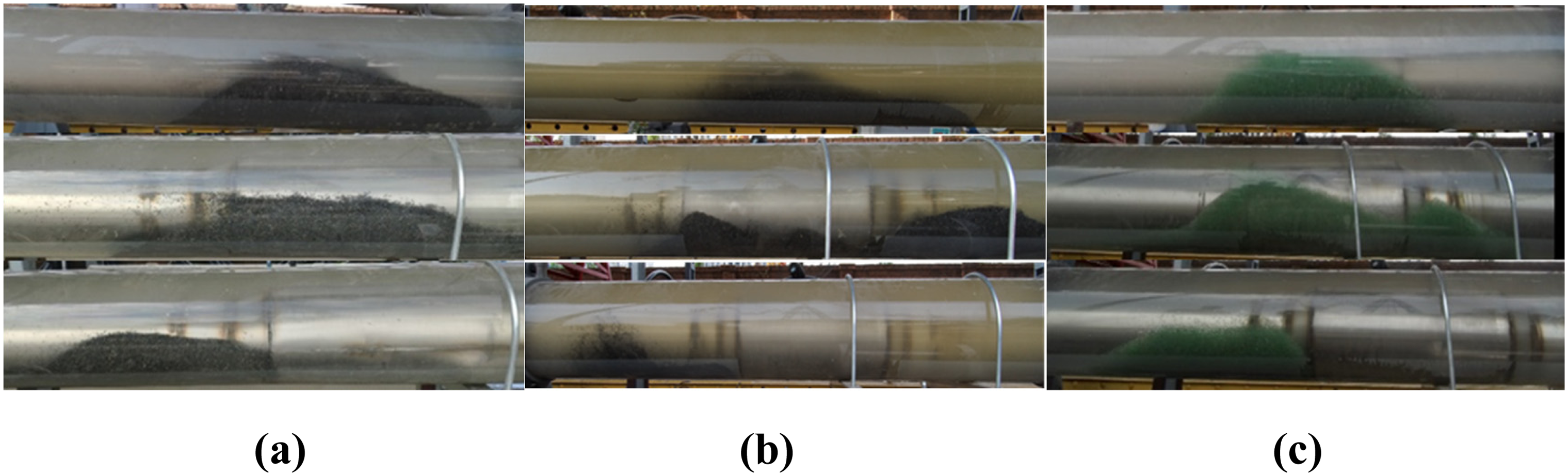
Comparison of experimental phenomena: (a) clean water; (b) simulated drilling fluid; (c) spherical cuttings.

Influence of drill pipe rotation speed on migration of cuttings

Figure 6(a) shows the influence of drill pipe rotation speed on cuttings removal time in different eccentric annuli. When the eccentricity was 0, the influence of rotation speed on cutting clearing time was not significant. When the rotation speed was increased from 10 to 50 rpm, the cuttings bed clearing speed increased by only <20%. When the eccentricity was 0.2 and 0.3 and the rotation speed was increased from 10 to 50 rpm, the cuttings bed clearing speed increased by >200%. Under the condition of eccentricity, increasing the rotation speed of the drill pipe has an obvious influence on the cuttings removal time. Because the drill pipe is in close contact with the cuttings at the bottom of the annulus, this enhances the agitation of the particles to transfer them to the area with higher fluid velocity. Figure 6(b) proves that higher fluid viscosity is beneficial to cuttings migration. Compared with clean water, the cuttings bed formed by the simulated drilling fluid is thinner, and the amount of cuttings carried by the annulus is greater.

Figure 6.

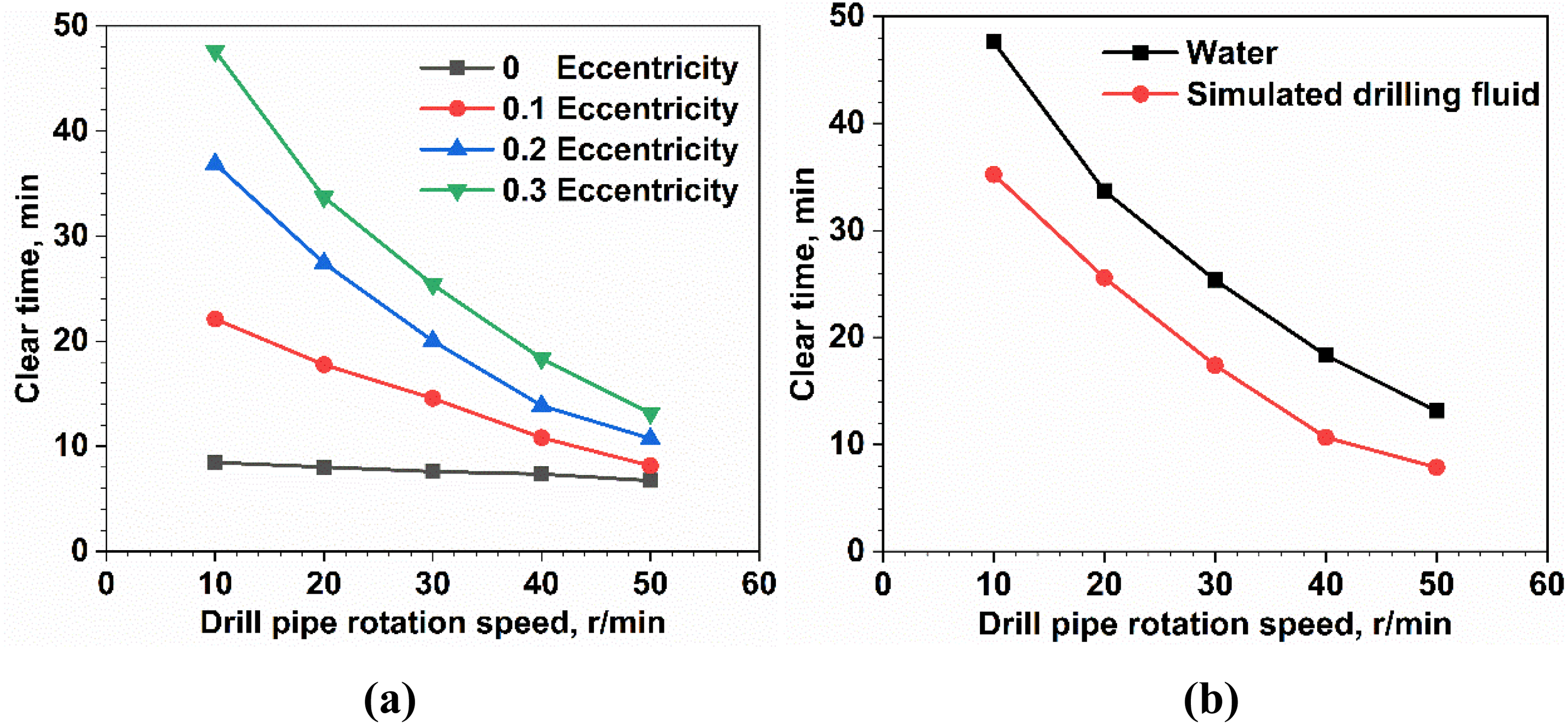
Influence of drill pipe rotation speed on cuttings clearing time: (a) clean water; (b) comparison between clean water and simulated drilling fluid.

Influence of drilling fluid displacement on migration of cuttings

Figure 7(a) shows the influence of drilling fluid displacement on cuttings removal time in different eccentric annuli. With the increase of displacement, the removal speed of cuttings under different eccentricities also accelerated. This is because, with the increase of fluid velocity, the shear stress acting on the cuttings bed increases, accelerating the migration of cuttings. Figure 7(b) shows the same result for the simulated drilling fluid.

Figure 7.

Influence of displacement on cuttings clearing time: (a) clear water; (b) comparison between clean water and simulated drilling fluid.

Comparison of flaky and spherical cuttings

Figure 8 shows that the clearing time of flaky cuttings is obviously inconsistent with that of spherical cuttings, indicating that there are differences in their migration modes. Spherical cuttings were removed an average of 66.7% faster than flaky cuttings, which is mainly because of their different stress and migration modes. Orthogonal analysis of the flaky cuttings reveals that the cuttings clearing time is influenced in order by the rotation speed, drilling fluid displacement, and eccentricity, with R²  =  95.5%.

Figure 8.

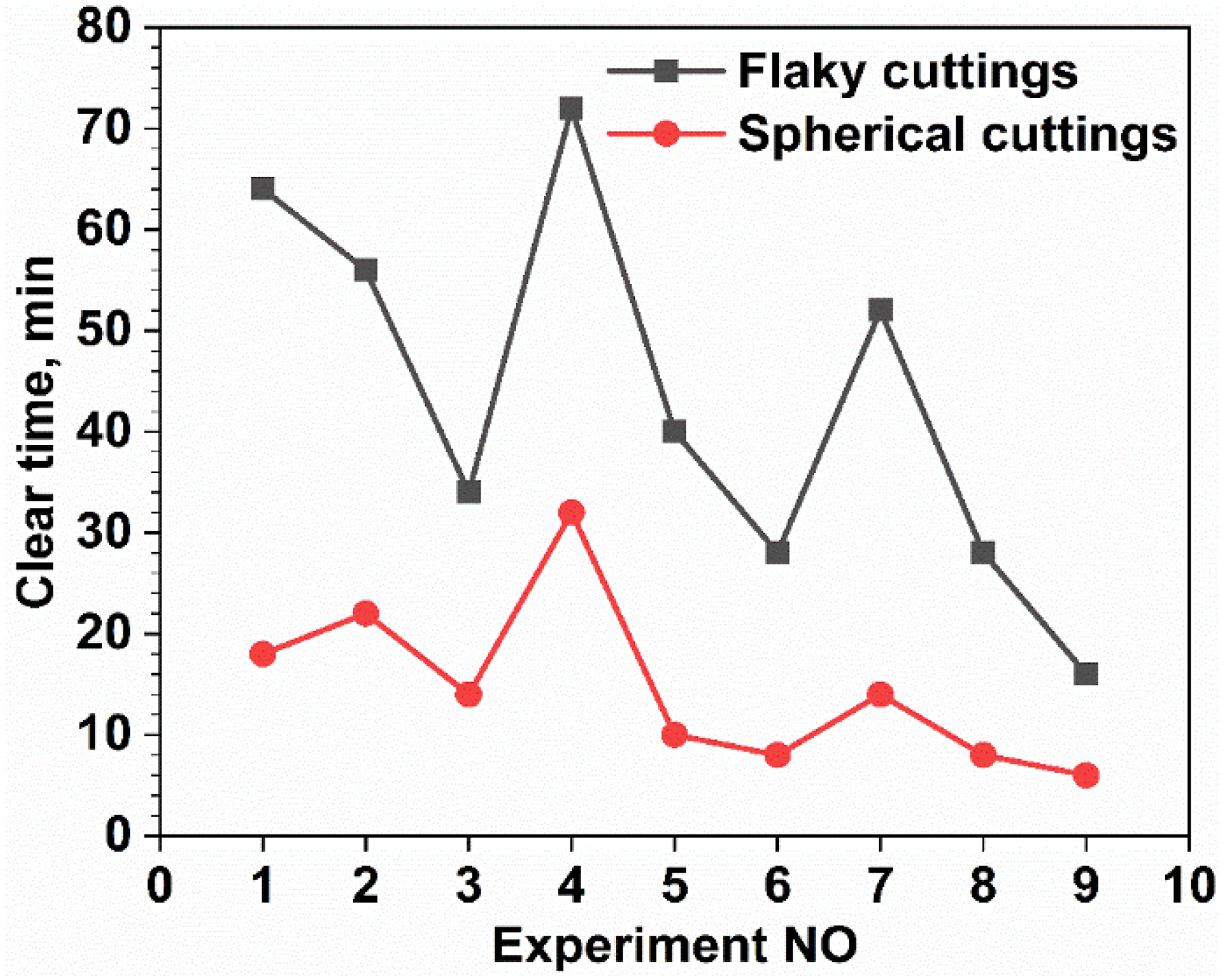
Comparison between flaky and spherical cuttings.

In other words, the rotation speed and drilling fluid displacement of the drill pipe are the main drilling parameters that affect hole cleaning. There are differences in the migration of flaky cuttings and spherical cuttings in the horizontal section, so it is necessary to study the migration of flaky cuttings in horizontal wells. Compared with clean water, the cuttings clearing speed was faster after using the simulated drilling fluid.

Numerical results and discussion

CFD model validation

The numerical simulation and experimental results of cuttings migration were verified, as shown in Figures 9 and 10. First, the horizontal annulus, drill pipe joint, and back end of the drill pipe joints were selected, and the cuttings migration phenomenon obtained from the simulation was compared with that obtained experimentally, as shown in Figure 9. There is good consistency between them. In the simulation diagram, the blue color indicates the drilling fluid and the red color indicates the cuttings bed. Figure 10 shows the comparison of simulation and experimental results. The average error between simulated and experimental drill pipe rotation speed was 15.8%, while that for drilling fluid displacement was 16.1%. The accuracy of the numerical model is therefore considered acceptable for engineering application and can be used in drilling engineering. Numerical simulation was then used to further study the influencing factors of cuttings bed thickness.

Figure 9.

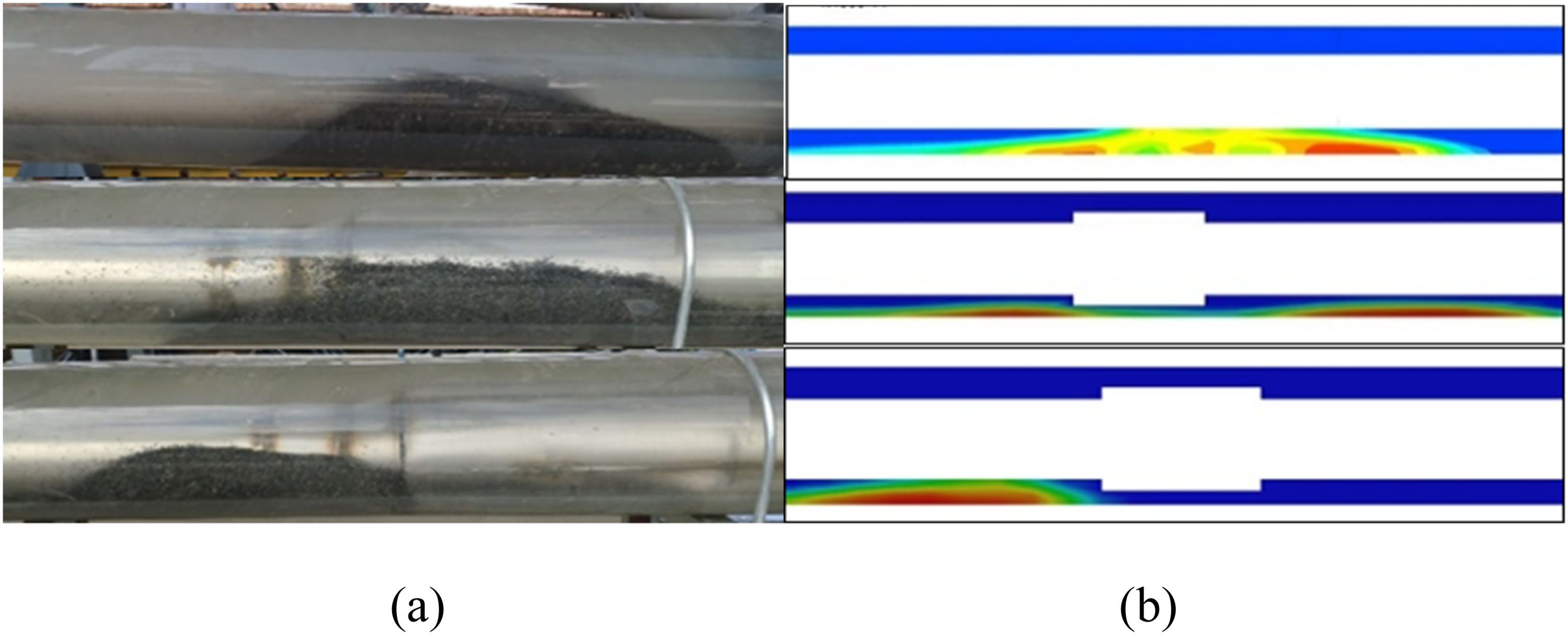
Comparison of (a) experimental phenomena and (b) simulated phenomena under the same conditions.

Figure 10.

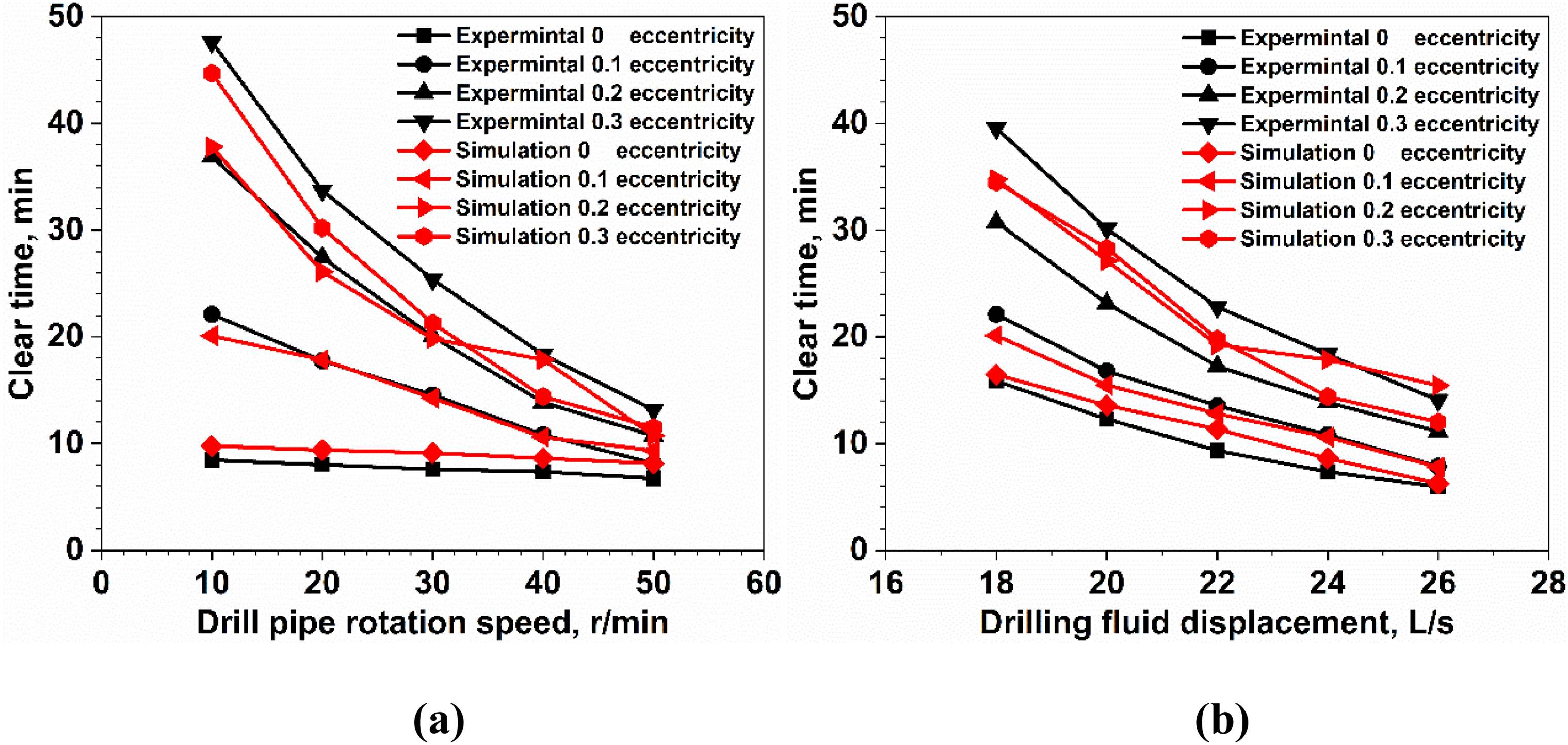
Influence of experimental and simulation results of (a) drill pipe rotation speed and (b) drilling fluid displacement on cuttings clearing time.

Influence of drilling fluid velocity

Figure 11 captures the nephograms of drilling fluid velocity of experiments 6 and 10, which can visually show the change of drilling fluid velocity inside the annulus. The middle part is the drill pipe, the rest is the drilling fluid (shown in red). It can be seen from the figure that the drilling fluid speed reached its maximum at the drill pipe joint. When the eccentricity was 0, the velocities of the annulus above and below the wellbore were basically equal. However, when the eccentricity was high, the velocity in the upper annulus was higher than that in the lower annulus. Because of the resistance caused by cuttings accumulation, the velocity near the bottom of the annulus was very small, so diagenetic cuttings can easily accumulate at the bottom of the annulus, as indicated by the experimental results.

Figure 11.

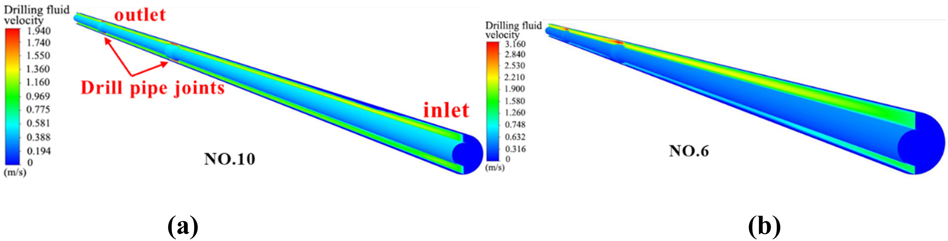
Velocity cloud charts of the drilling fluid for (a) experiment 6 and (b) experiment 10.

Influence of drill pipe rotation speed

Figure 12 shows cross-sectional views of the annulus for five rotation speeds and 15 groups of simulation phenomena; the blue part is the drilling fluid and the red part is the cuttings bed. The higher the rotation speed, the greater the height of the cuttings bed. When the rotation speed was 30 rpm, the cuttings bed basically moved at the bottom of the wellbore, as shown in Figure 12(a). With the increase of rotation speed, the migration position of the cuttings bed gradually became higher, as shown in Figure 12(b)–12(d). When the rotation speed reached 122 rpm, the cuttings bed reached the middle of the annulus, as shown in Figure 12(e). When the rotation speed of the drill pipe increased, higher shear gets applied to the fluid, which enhances the agitation of the particles to drive them upward. The height of the annular cuttings bed is affected not only by the rotation speed but also by eccentricity, physical properties, and the displacement of the drilling fluid. The greater the eccentricity, the greater the height of the cuttings bed. This is because the drill pipe will be in close contact with the cuttings bed at the bottom of the annulus, and the rotation of the drill pipe will produce a spiral flow, which will entrain the cuttings particles, so that more cuttings will accumulate along the borehole wall.

Figure 12.

Sectional views of the annulus with drill pipe rotation speeds of (a) 30, (b) 53, (c) 76, (d) 99, and (e) 122 rpm.

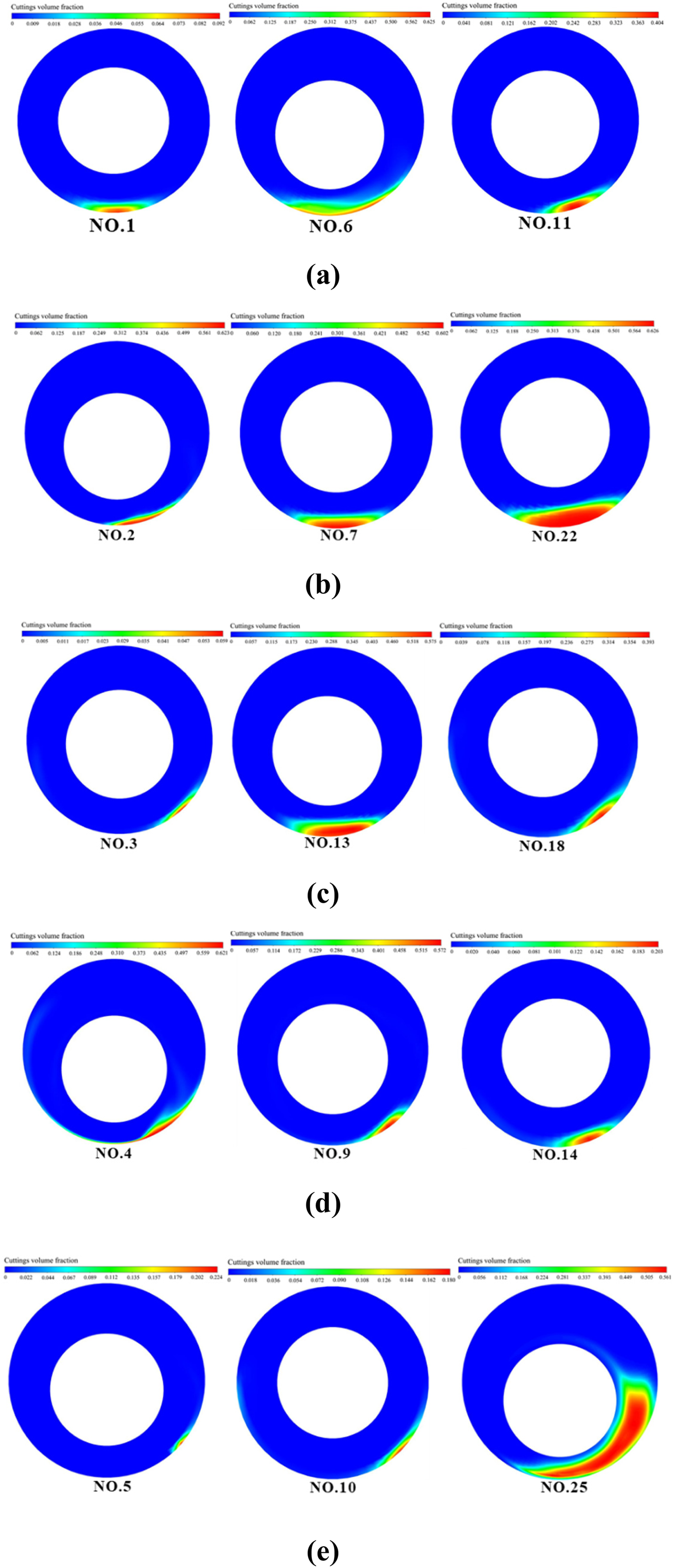
Figure 13 shows the distribution position of the cuttings bed in the horizontal annulus. With the increase of drill pipe rotation speed, more cuttings will be driven, and under the combined action of the drilling fluid, the cuttings bed will move along the borehole wall (e.g. experiments 3, 5, and 18). This demonstrates that the cuttings bed can more easily be removed under the combined action of drill pipe rotation speed and drilling fluid. When the rotation speed is low, the cuttings bed mainly accumulates at the bottom of the annulus (e.g. experiments 1, 6, and 7). When the displacement of the drilling fluid is large, there is almost no cuttings bed accumulation in the annulus, and only a small amount of cuttings accumulates at the back end of the drill pipe joint (e.g. experiments 2). When the eccentricity is large, the cuttings bed distribution oscillates at the bottom of the annulus, and the cuttings bed spreads to both sides of the borehole wall. This is because the drill pipe is in close contact with the cuttings bed at the bottom of the annulus at this time, and there is less space at the bottom of the annulus (e.g. experiments 15).

Figure 13.

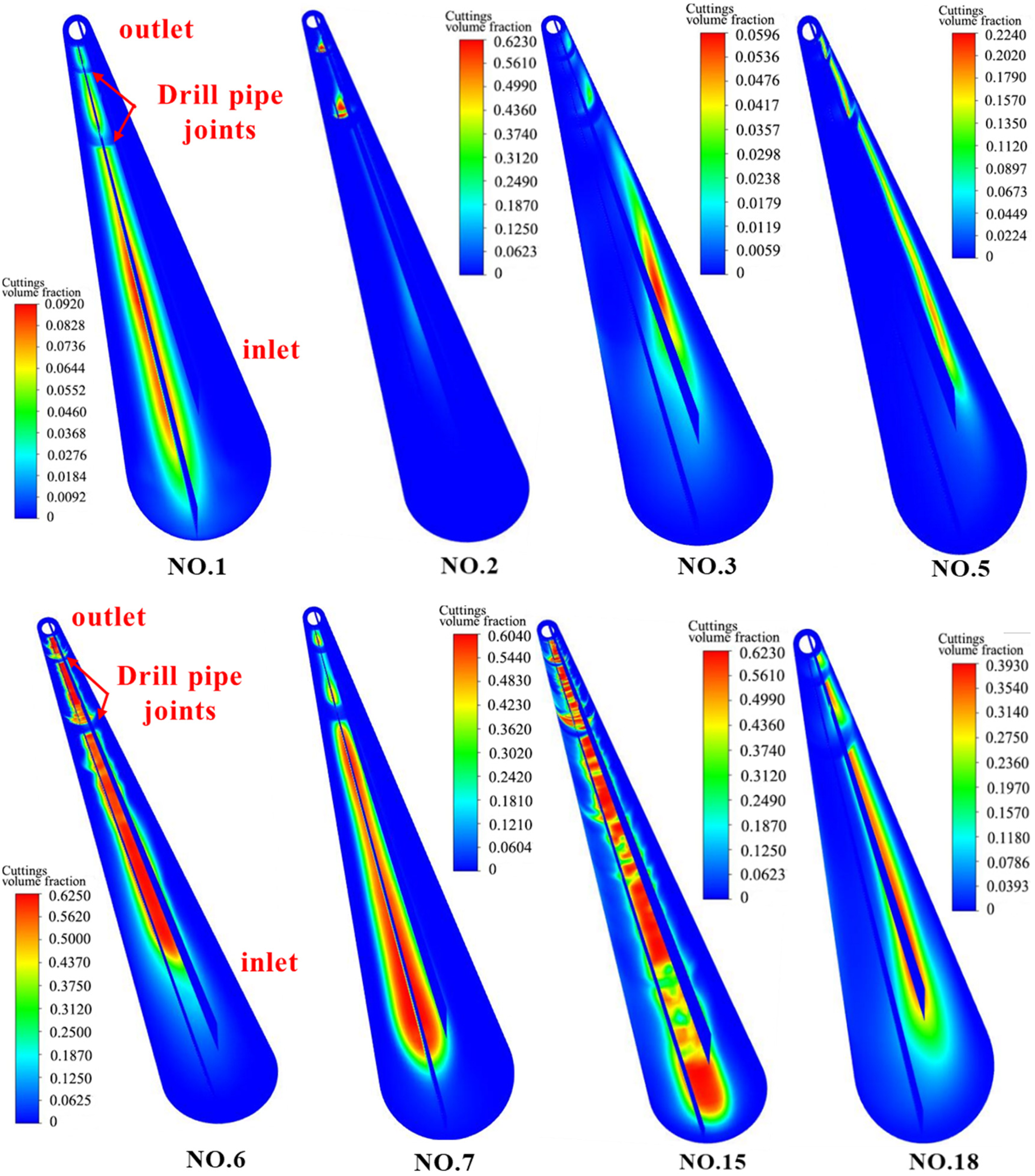
Distribution of cuttings bed in the horizontal annulus.

Empirical model

Figure 14 shows the simulation results of cuttings bed thickness. The results are based on the intercept of the cross section of the annulus where the volume fraction of the cuttings bed is the largest in the simulation results, taking the volume fraction of 10% as the minimum value, and we use the Pythagorean theorem to calculate the place where the thickness of the cuttings bed is the largest The simulated data were then compared with 10% of the wellbore diameter (Wang et al., 2011), and the line formed by 10% of the wellbore diameter is referred to as the safety line of the cuttings bed. Beyond this line, it is considered that there is a safety risk under this working condition parameter.

Figure 14.

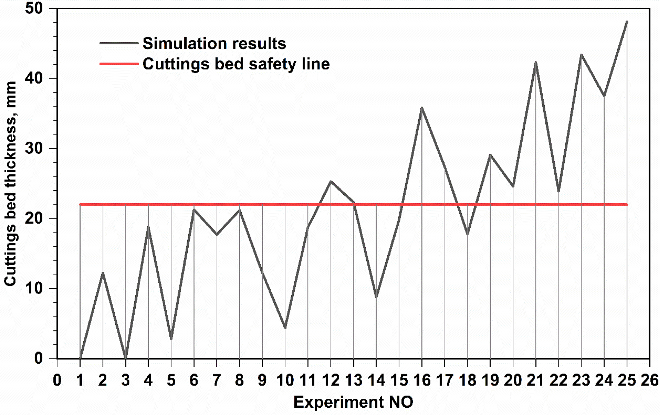
Simulated data of cuttings bed thickness.

Based on 25 sets of simulation data of cuttings bed thickness, the Wang model (Wang et al., 1993) can be modified as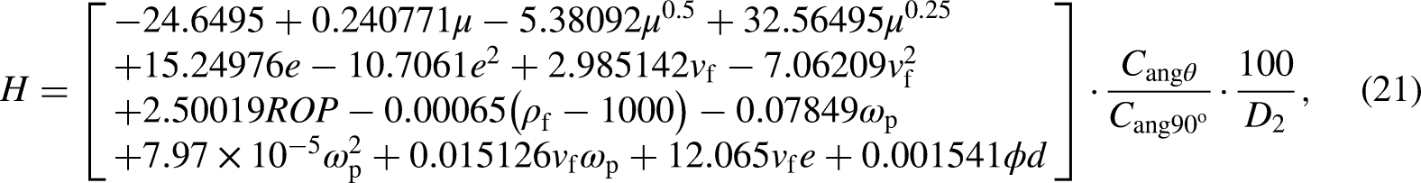

$$H=\left[\begin{array}{c}-24.6495+0.240771\mu -5.38092{\mu }^{0.5}+32.56495{\mu }^{0.25}\\ +15.24976e-10.7061e^2+2.985142v_{\mathrm{f}}-7.06209v_{\mathrm{f}}^2\\ +2.50019ROP-0.00065\left({\rho }_{\mathrm{f}}-1000\right)-0.07849{\omega }_{\mathrm{p}}\\ +7.97\times {10}^{-5}{\omega }_{\mathrm{p}}^2+0.015126v_{\mathrm{f}}{\omega }_{\mathrm{p}}+12.065v_{\mathrm{f}}e+0.001541\varphi d\end{array}\right]\cdot {\displaystyle \frac{C_{\mathrm{ang}\theta }}{C_{\mathrm{ang}{90}^{\mathrm{o}}}}\cdot {\displaystyle \frac{100}{D_2},}}$$

(21)

where H (%) is the thickness of the dimensionless cuttings bed, ROP (m/h) is the penetration rate, ω_p (rpm) is the rotation speed of the drill pipe, $C_{\mathrm{ang}\theta }=0.0342\theta -0.000233{\theta }^2-0.213$ is the angle of inclination correction coefficient of $\theta$ , where $\theta$ (degrees) is angle of inclination, and $C_{\mathrm{ang}{90}^{\mathrm{o}}}$ is the angle of inclination correction coefficient of 90°.

The Wang model was put forward according to the results of his experiments, in which factors such as drilling fluid displacement, drilling fluid density, drilling fluid viscosity, eccentricity, rotation speed, and cuttings injection speed were considered. Because his model is only suitable for spherical cuttings and does not consider the influence of cuttings size and angle of inclination, the model has limitations. In this study, his model was modified by multiple nonlinear mathematical regression, and the influence of angle of inclination was considered. The calculation process is shown in the Appendix.

For a Bingham fluid, the effective viscosity in can be calculated by using Eq. (22).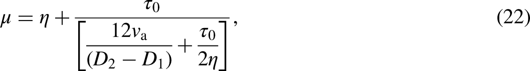

$$\mu =\eta +{\displaystyle \frac{{\tau }_0}{\left[{\displaystyle \frac{12v_{\mathrm{a}}}{(D_2-D_1)}+{\displaystyle \frac{{\tau }_0}{2\eta }}}\right]},}$$

(22)

and, for a power-law fluid, the effective viscosity can be calculated by using Eq. (23).

$$\mu =K{\left({\displaystyle \frac{2n+1}{3n}}\right)}^n(D_2-D_1{)}^{1-n}(12v_{\mathrm{a}}{)}^{n-1},$$

(23)

where $\eta$ (mPa⋅s) is the plastic viscosity of the Bingham fluid, ${\tau }_0$ (Pa) is the dynamic shear force of the Bingham fluid, $v_{\mathrm{a}}$ (m/s) is the average return velocity of the annular drilling fluid, K (Pa⋅s ⁿ ) is the consistency coefficient of the power-law fluid, and n is the power-law fluid fluidity index (dimensionless).

To verify the accuracy of this model, the calculation results of the fitting formula were compared with the simulation results, as shown in Figure 15(a). The coefficient of determination was R²  =  0.973. To further verify the accuracy of this model, the classic model (Wang et al., 1993; Yang et al., 2008) was used to compare with this model, as shown in Figure 15(b). Although there are some deviations in the comparison results, the overall trend is consistent. Except for experiments 7 and 23 in this model, the thickness of the other cuttings beds was greater than the calculation results of the Wang and Yang models, demonstrating that there are differences between the models of flaky cuttings and spherical cuttings, with flaky cuttings more easily accumulated, which can also be proved by experiments.

Figure 15.

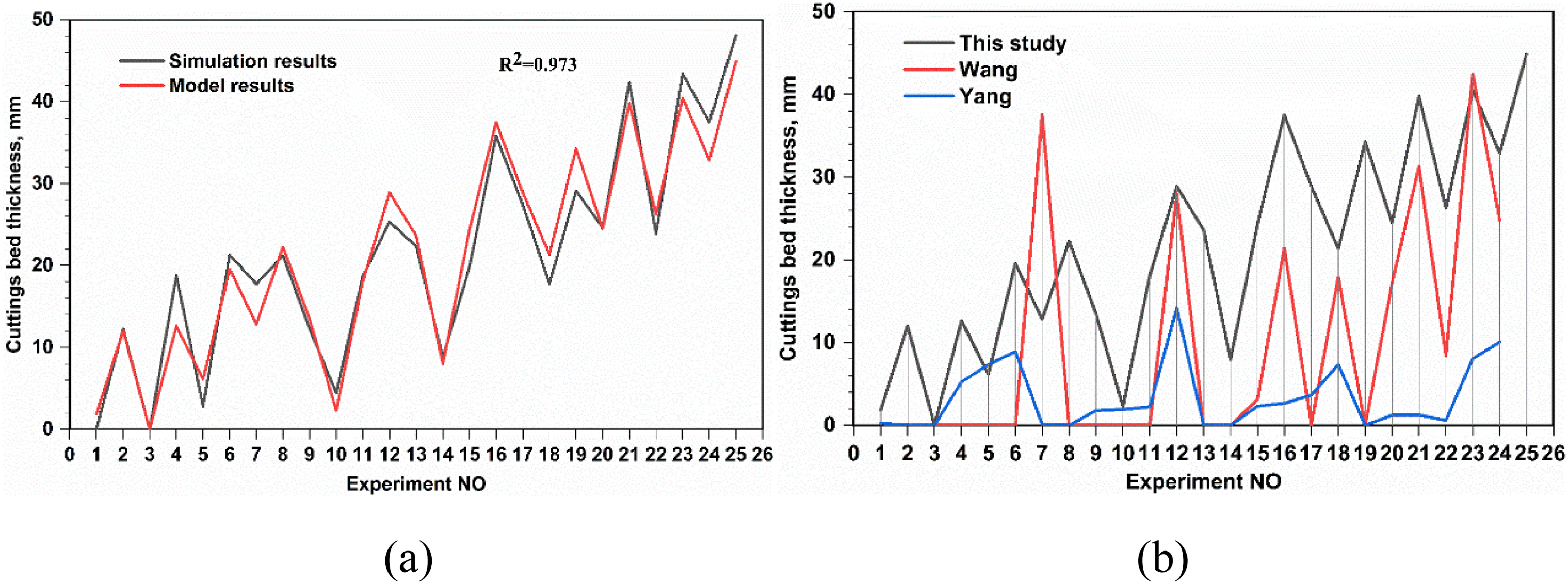
Model validation, showing comparison with (a) simulated results and (b) classic models.

Example analysis of optimization of hole cleaning process parameters

Sensitivity analysis

Using the model in this study, various technological parameters were varied in turn, and the influence of each parameter on the dimensionless cuttings bed thickness was analyzed. According to the process parameters of typical shale gas wells, the calculation parameters were selected as follows: borehole diameter  =  220 mm, drill pipe diameter  =  127 mm, ROP  =  8 m/h, angle of inclination  =  90°, equivalent diameter of cuttings  =  1.24 mm, drilling fluid density  =  1900 kg/m³, plastic viscosity  =  40 mPa⋅s, dynamic shear force  =  10 Pa, drilling fluid displacement  =  30 L/s, and eccentricity  =  0.4. The results are shown in Figure 16.

Figure 16.

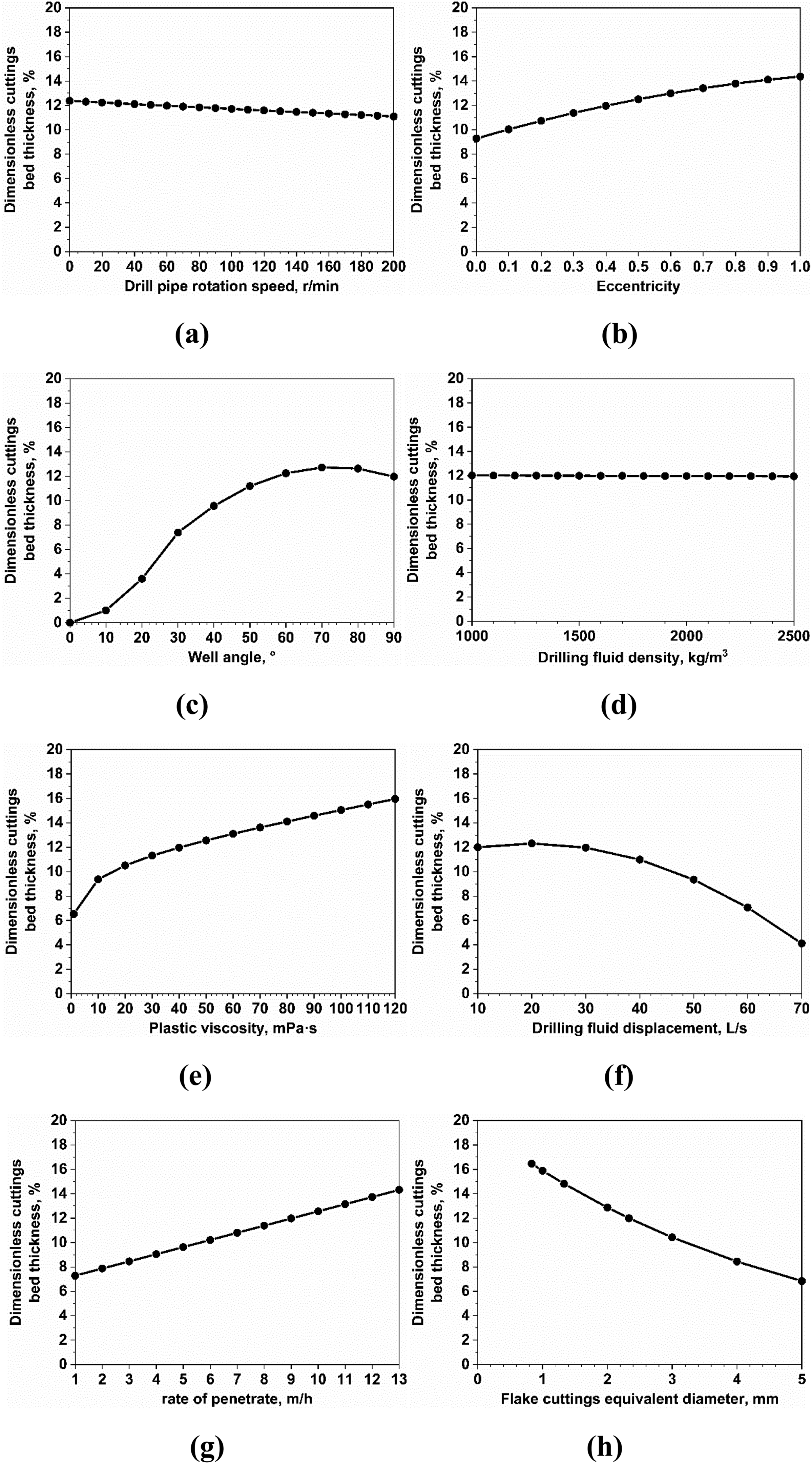
Sensitivity analysis of dimensionless cuttings bed thickness, showing the influence of (a) drill pipe rotation speed, (b) eccentricity, (c) angle of inclination, (d) drilling fluid density, (e) plastic viscosity of the drilling fluid, (f) displacement, (g) penetration rate, and (h) equivalent diameter of cuttings.

Figure 16(a) shows the influence of drill pipe speed. The greater the rotation speed, the thinner the cuttings bed. When the drill pipe does not rotate, its dimensionless cuttings bed thickness can reach 12.4%, and when it was increased to 200 rpm, its dimensionless cuttings bed thickness dropped to 11.1%. The main reason for this is that the rotation of the drill pipe increases the swirling degree of the drilling fluid in the annulus. Therefore, increasing the rotation speed of the drill pipe has a certain effect on hole cleaning.

Figure 16(b) shows the influence of eccentricity. With the increase of eccentricity, the thickness of the cuttings bed increased greatly. When eccentricity was 0, its dimensionless cuttings bed thickness was 9.3%, and, when eccentricity was increased to 1, its dimensionless cuttings bed thickness increased to 14.4%. In horizontal well drilling, because of gravity, drilling tools tend to lie on the lower side of the borehole, resulting in an uneven distribution of the annulus, forming two areas with different flow cross-sectional areas, hindering hole cleaning. The reason for this phenomenon lies in the uneven distribution of drilling fluid velocity in the annulus caused by eccentricity, the low velocity in the narrow gap at the lower part of the annulus, and the weak ability to carry cuttings. The velocity at the wide gap in the upper annulus is high, and the ability of carrying cuttings is strong. Moreover, because of gravity, cuttings tend to gather in the lower part of the annulus, further aggravating the accumulation of cuttings. Therefore, the greater the eccentricity, the weaker the ability to carry cuttings, and the greater the thickness of the cuttings bed. Therefore, controlling eccentricity has discernable effect on hole cleaning.

Figure 16(c) shows the effect of inclination angle. As the inclination angle of the well is increased, the thickness of the cuttings bed first increases and then decreases. When the inclination angle was 10°, the thickness of the dimensionless cuttings bed was 1.0%; when the inclination angle was increased to 70°, the thickness of the dimensionless cuttings bed was 12.7%; and when the inclination angle was 90°, the dimensionless cuttings bed thickness was 11.9%. Therefore, an inclination angle 70° makes it the most difficult section to carry cuttings. The transport of cuttings in the annulus of highly deviated wells is controlled by a rolling mechanism, making it more difficult to carry cuttings than in vertical and horizontal wells.

Figure 16(d) shows the influence of drilling fluid density. With the increase of drilling fluid density, the thickness of the cuttings bed barely changes. When the density of drilling fluid was 1000 kg/m³, its dimensionless cuttings bed thickness was 12.0%; when it was increased to 2500 kg/m³, its dimensionless cuttings bed thickness dropped to 11.9%. Therefore, changing the density of drilling fluid barely changes the thickness of the cuttings bed.

Figure 16(e) shows the influence of the plastic viscosity of the drilling fluid. With the increase of plastic viscosity, the thickness of the cuttings bed also increases. When the plastic viscosity was 1–10 mPa·s, the thickness of the cuttings bed increased considerably compared with other situations. There is an overall increasing trend. Therefore, properly reducing the plastic viscosity of the drilling fluid has a discernable effect on hole cleaning.

Figure 16(f) shows the influence of drilling fluid displacement. With the increase of displacement, the thickness of the cuttings bed first increases and then decreases. When the displacement was 20 L/s, the dimensionless cuttings bed thickness was the greatest (12.3%). When it was increased to 70 L/s, its dimensionless cuttings bed thickness was reduced to 4.1%. The reason for this difference is that, with the increase of displacement, the return velocity of the annulus increases, which increases the turbulence of the drilling fluid in the annulus. Therefore, increasing the circulating displacement of the drilling fluid has a discernable effect on hole cleaning.

Figure 16(g) shows the influence of the ROP. The greater the ROP, the greater the thickness of the cuttings bed. When the ROP was 1 m/h, the dimensionless cuttings bed thickness was 7.3%, and, when it was increased to 13 m/h, the dimensionless cuttings bed thickness increased to 14.3%. The reason for this difference is that the increase in the ROP leads to the increase of cuttings in the wellbore annulus, and the untimely removal of cuttings thickens the cuttings. Therefore, proper control of the ROP has a slight effect on hole cleaning.

Figure 16(h) shows the influence of cuttings size. The larger the equivalent diameter of cuttings, the smaller the thickness of the cuttings bed. When the equivalent diameter of the cuttings was 0.833 mm, its dimensionless cuttings bed thickness was 16.5%, and, when it was increased to 5 mm, its dimensionless cuttings bed thickness dropped to 6.8%. The equivalent diameter of cuttings is closely related to bit type, rock type, weight on bit, drill pipe speed, and cuttings migration efficiency. In the selected cuttings diameter range, small cuttings are more difficult to migrate than large cuttings. This is because small-sized cuttings are easier to gather and the force between particles is greater.

Field application

The Changning 209H24-1 well is a horizontal shale gas development well with a long horizontal section. The Changning 209H24-1 well is located in Group 5, Xiaozhai Village, Daba Miao Township, Xingwen County, Yibin City, Sichuan Province, China. On July 6, 2021, the well depth was drilled to 2760 m, the cuttings return was not obvious, and the friction torque of the drill string was large. Analysis of the distribution of the cuttings bed in this well by using the model in this study indicated that there was a cuttings bed in the 2760–4500 m well section and the accumulation of the cuttings bed in the 2820–3000 m well section was particularly obvious. Therefore, it is necessary to optimize the process parameters of this well.

Basic information

The Changning 209H24-1 well has a design depth of 4500 m, a vertical depth of 2733 m, a target point A at a depth of 3000 m. The third section of the well is at a depth of 500–1397 m, its hole size is Φ311.2 mm  ×  1397 m, and the casing size is Φ244.5 mm  ×  1395 m; the fourth well section of the well is at a depth of 1397–4500 m, and its hole size is Φ215.9 mm  ×  4500 m. The density of the Bingham drilling fluid used was 1970–2320 kg/m³, its plastic viscosity was 28–80 mPa⋅s, and the dynamic shear force was 5–15 Pa. According to the drilling parameters, the minimum rotation speed was 80 rpm, the minimum displacement was 35 L/s, the ROP was 10 m/h, and the eccentricity was ∼0.5.

Prediction of cuttings bed thickness

Figure 17 shows the thickness of the cuttings bed in the whole well section calculated according to the model in this study. The calculation parameters were as follows: density of drilling fluid  =  1970 kg/m³, plastic viscosity of the fluid  =  28 mPa⋅s, dynamic shear force  =  5 Pa, rotation speed  =  80 rpm, displacement  =  35 L/s, ROP  =  10 m/h, and eccentricity  =  0.5. When drilling according to these parameters, the cuttings carried in the wellbore were not smooth, and the hole cleaning was poor. The thickest cuttings bed appeared at a well depth of ∼2910 m, at which point the angle of inclination was 74° and the thickness of cuttings bed was 26.8 mm. In the horizontal section of 3000–4500 m, the thickness of the cuttings bed was as high as 25.2 mm, which means that the annulus had been blocked. Therefore, it is necessary to adjust the drilling parameters or drilling fluid properties to improve hole cleaning.

Figure 17.

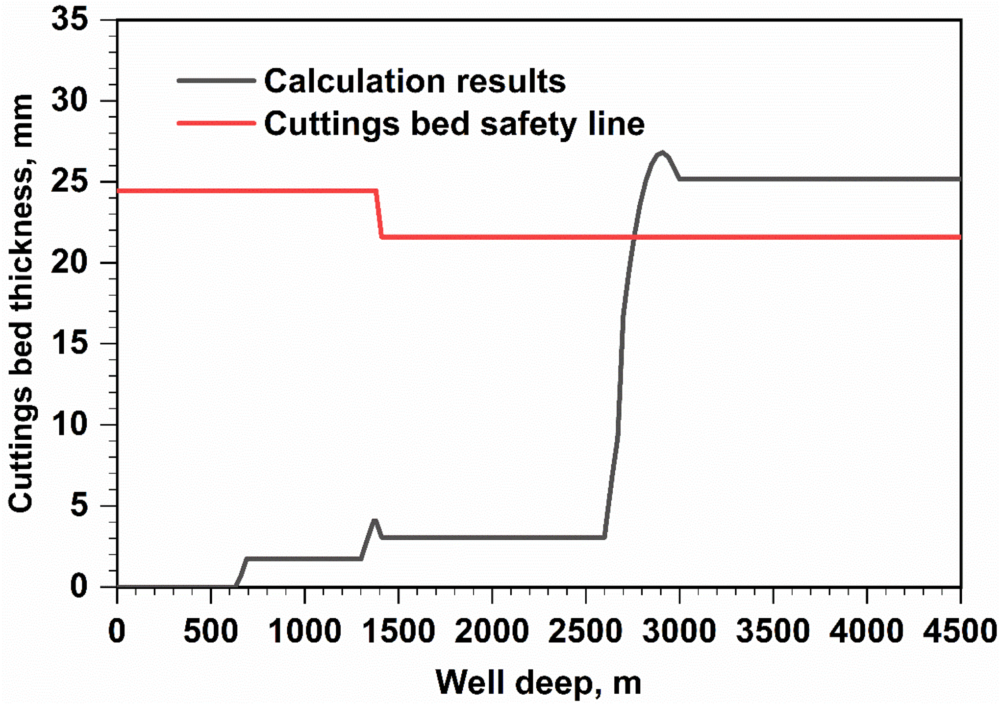
Thickness of cuttings bed in different well sections.

Optimization of process parameters

Figure 18 shows the optimization of process parameters. Figure 18(a) shows the influence of changing the drilling fluid displacement. The thickness of the cuttings bed can be significantly reduced by increasing the displacement of the drilling fluid. When the displacement of the drilling fluid was increased to 40 L/s, the maximum thickness of the cuttings bed at a depth of ∼2910 m was 25.4 mm. When the displacement of drilling the fluid continued to increase to 50 L/s, the maximum thickness of the cuttings bed was only 21.4 mm, which is lower than the safety line of cuttings bed thickness, and it can be considered that hole cleaning efficient. However, displacement of the drilling fluid was 50 L/s, which is a large displacement in engineering applications and may cause other engineering problems.

Figure 18.

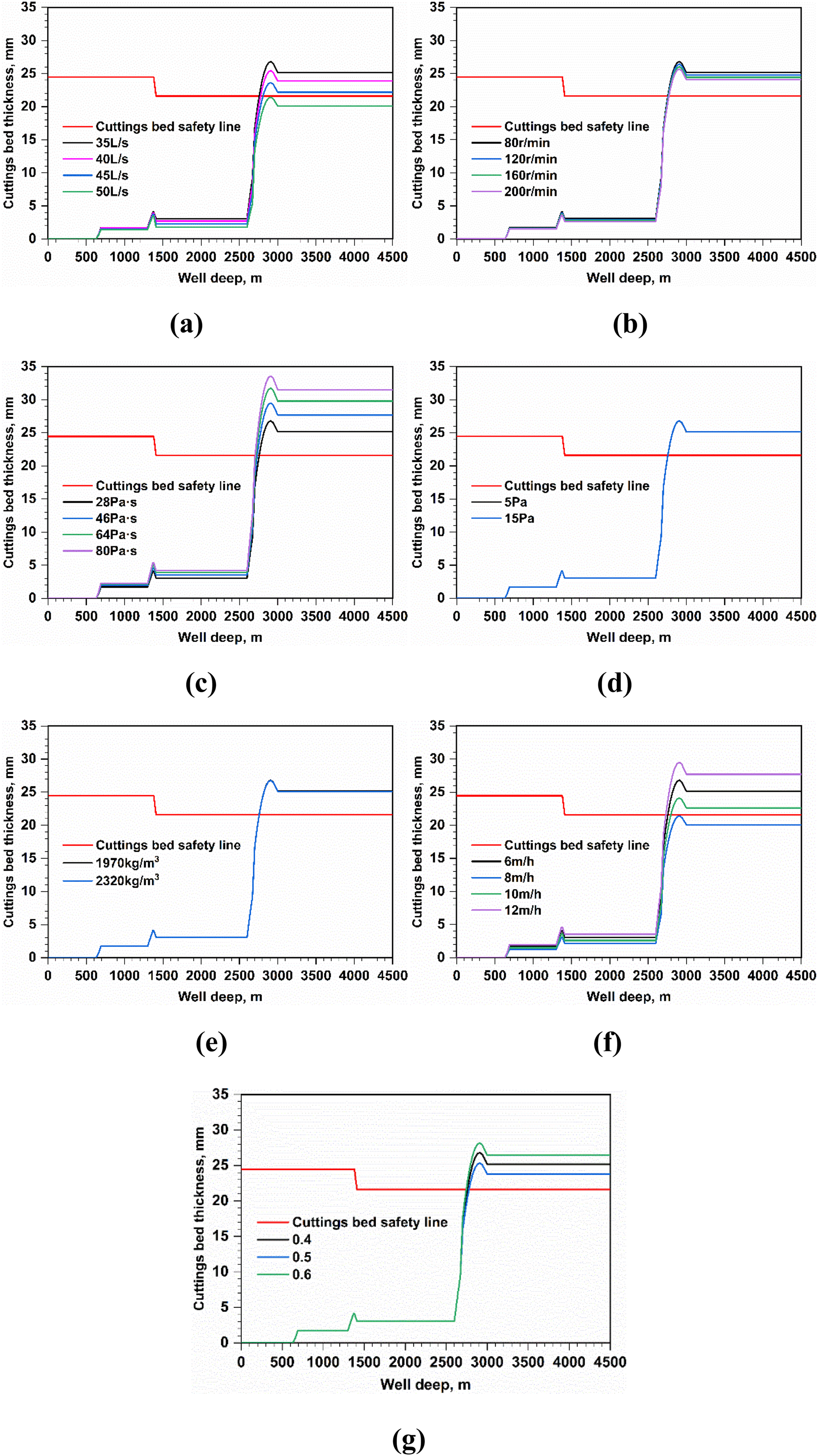
Optimization Of process parameters with changes in the (a) displacement of the drilling fluid, (b) rotation speed of the drill pipe, (c) plastic viscosity of the drilling fluid, (d) dynamic cutting force of the drilling fluid, (e) density of the drilling fluid, (f) penetration rate, and (g) eccentricity.

Figure 18(b) shows the influence of changing the speed of the drill pipe. The thickness of the cuttings bed cannot be significantly reduced by increasing the rotation speed. Even when the rotation speed was increased to 200 rpm, the maximum thickness of the cuttings bed was 25.7 mm, which is still higher than the safety line of cuttings bed thickness. Therefore, the thickness of the cuttings bed cannot be obviously reduced by changing the rotation speed alone, but it needs to be changed together with other parameters.

Figure 18(c) shows the influence of changing the plastic viscosity of the drilling fluid. The thickness of the cuttings bed can be significantly changed by changing the plastic viscosity of the drilling fluid. When the plastic viscosity of the drilling fluid was increased to 80 Pa⋅s, the thickness of the cuttings bed was 33.6 mm, which is much higher than the safety line of cuttings bed thickness, so the plastic viscosity of the drilling fluid should be reduced. However, in this study, the plastic viscosity of the drilling fluid reached a minimum value. Therefore, changing the plastic viscosity of the drilling fluid was not considered when changing the process parameters.

Figure 18(d) shows the influence of changing the dynamic shear force of the drilling fluid. Figure 18(e) shows the influence of changing the density of the drilling fluid. By changing these two parameters, the thickness of cuttings bed barely changes. Therefore, changing these two parameters was not considered when changing the process parameters.

Figure 18(f) shows the influence of changing the ROP. The thickness of the cuttings bed can be significantly reduced by changing the ROP. When the ROP was increased to 12 m/h, the maximum cuttings bed thickness was 29.5 mm, which is far higher than the safety line of cuttings bed thickness. When it was reduced to 6 m/h, the thickness of the cuttings bed was lower than the safety line, and it can be considered that hole cleaning was efficient. However, too low an ROP will affect the project progress, thus affecting the economic cost of the project.

Figure 18(g) shows the influence of changing eccentricity. The thickness of the cuttings bed can be significantly reduced by changing eccentricity. When the eccentricity was increased to 0.6, the maximum thickness of cuttings bed was 28.2 mm, which is much higher than the safety line of cuttings bed thickness. When it was reduced to 0.4, the maximum thickness of the cuttings bed was 25.3 mm. Therefore, reducing eccentricity can reduce the thickness of the cuttings bed. Eccentricity cannot easily be changed in the horizontal section of a horizontal well, but it can be reduced by adding centralizers.

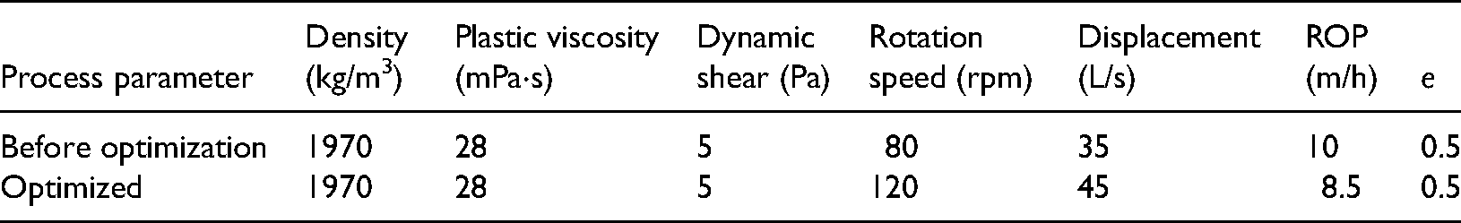
Through the analysis of the above seven technological parameters, if the thickness of cuttings bed during drilling in the Changning 209H24-1 well is to be reduced to below the safety line of cuttings bed, then the operating parameters need to be adjusted as follows: rotation speed increased to 120 rpm, displacement increased to 45 L/s, and penetration rate decreased to 8.5 m/h, with other parameters remaining unchanged, as listed in Table 4. For this situation, the thickness of the cuttings bed is shown in Figure 19. After comprehensively changing the working condition parameters, the thickness of the cuttings bed was made to be lower than the safety line of cuttings bed thickness, and the hole cleaning condition was good. Drilling under these working condition parameters will not cause sticking risk. After predicting the thickness of the cuttings bed by using the model and adjusting the working conditions, there were no complicated downhole accidents in the well during drilling and cuttings returned smoothly, which was in line with the prediction of the model.

Figure 19.

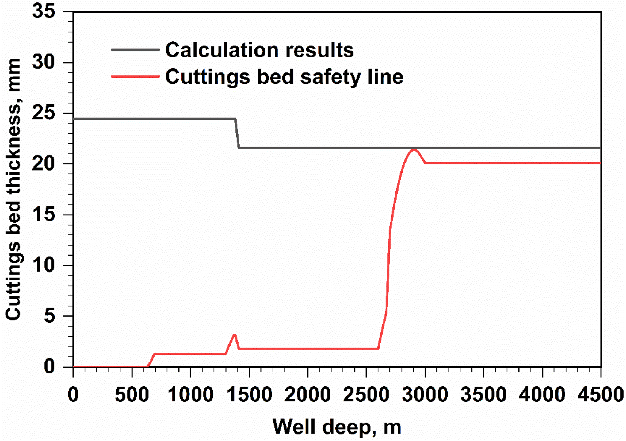
Thickness of cuttings bed in different well sections after changing parameters.

Table 4.

Parameters before and after optimization.

Process parameter	Density (kg/m3)	Plastic viscosity (mPa⋅s)	Dynamic shear (Pa)	Rotation speed (rpm)	Displacement (L/s)	ROP (m/h)	e
Before optimization	1970	28	5	80	35	10	0.5
Optimized	1970	28	5	120	45	8.5	0.5

Conclusions

In this study, the migration law of flaky cuttings in horizontal wells is studied through simulation calculation and experimental verification. A model for the distribution of a flaky cuttings bed in a long horizontal well considering many factors was put forward and applied in Well Ning 209H24-1. The conclusions can be summarized as follows.

The migration speed of flaky cuttings is different from that of spherical cuttings, and spherical cuttings are removed an average of 66.7% faster than flaky cuttings.

A distribution model of a long horizontal section flaky cuttings bed was proposed considering multiple factors, and the coefficient of determination was R²  =  0.973. There is a difference between this model and the classical model, indicating that the model of flaky cuttings established in this study is different from the model of spherical cuttings.

The rotation speed of the drill pipe, density of the drilling fluid, displacement of the drilling fluid, and equivalent diameter of cuttings all decreased with the increase of parameters, whereas the eccentricity, angle of inclination, plastic viscosity, and ROP all increased with the increase of parameters. Changing the drilling fluid density had little effect.

The application of this model in the Changning 209H24-1 well can be used to accurately calculate the thickness distribution of the cuttings bed in each well section and adjust the parameters to make the thickness of cuttings bed lower than the safety line of the cuttings bed. The calculated results are in good agreement with the actual drilling process of this well.

The model proposed in this study provides a good reference for predicting the thickness distribution of the cuttings bed and judging whether there is a risk of sticking during the drilling process. This model should be mainly used in drilling design, not after problems are encountered during the drilling process. In drilling engineering, the process parameters that can be changed and their scope are limited. To improve hole cleaning, further studies on wellbore structure, wellbore trajectory, and drilling tools are required.