Sage Journals: Discover world-class research

Abstract

In order to enhance the adaptability of energy management strategy (EMS) to complex and changeable driving cycles, this paper proposed an adaptive energy management strategy (A-EMS) based on intelligent recognition of driving cycle (IRDC) by the back propagation neural network (BPNN) and genetic algorithm (GA). Firstly, BPNN is employed to design IRDC. Secondly, the equivalent fuel consumption minimization strategy (ECMS) is derived based on Pontryagin's minimum principle (PMP). Then, GA is used to optimize the MAP of the initial equivalent factor (EF) with the initial state of charge (SOC) and mileage. At the same time, the SOC penalty function and the velocity penalty function are employed to modify the initial EF, and then an adaptive minimum equivalent fuel consumption strategy (A-ECMS) is established. Finally, A-ECMS strategy model based on IRDC is modelled by the Matlab/Simulink software, and its model control effect is verified. Simulation results show that compared with ECMS strategy, A-ECMS strategy can maintain high fuel economy under complex driving cycles, and improve the vehicle's fuel economy up to 3%.

Keywords

plug-in hybrid electric vehicles (PHEVs)adaptive equivalent consumption minimization strategy (A-ECMS)intelligent recognition of driving cycle (IRDC)back propagation neural network (BPNN)genetic algorithm (GA)

Introduction

Currently, EMS is still the focus of hybrid electric vehicle research, which has developed from single objective and single system to multi-objective integrated optimization and multi-system information sharing, as well as from rule-based (RB) EMS to intelligent EMS (Bayindir et al., 2011; Serrao et al., 2009; Zhang et al., 2015).

EMSs can be divided into RB-EMS (Sabri et al., 2016), global optimization EMS (Wang et al., 2019), instantaneous optimization EMS (Sun et al., 2017) and intelligent EMS (Wang et al., 2020).

RB-EMS is mainly designed according to characteristics of power components such as engines and motors in the power system (Zeman, 2014), while the optimized EMS mainly regards the energy distribution problem of power system as a mathematical problem with constraints to find the extremum, and then uses the corresponding optimization control theory to continuously improve RB-EMS, so that under predifined driving cycles, overcome the disadvantage of poor adaptability of RB-EMS, improve the fuel economy of vehicle in different driving cycles (Trovão et al., 2013).

RB-EMS has the advantages of simple design, fast response, robustness (Bayindir et al., 2011). Banvait H et al. designed the vehicle controller based on the fixed logic threshold value, and realized the torque distribution and mode switching of the vehicle (Banvait et al., 2009). Montazeri-Gh et al. (2006) used GA to optimize engine torque, took the lowest fuel and emission as the optimization objective, optimized RB-EMS in a city cycle, and fuel consumption was reduced by 4.7%. However, the result is optimal only in this condition. When the driving cycle changes, the selection of threshold is not optimal, and fuel consumption may become worse. Therefore, RB-EMS still needs to be improved.

Global optimization strategy is a kind of reverse optimization strategy, which can make vehicle optimally distribute power battery energy in a given driving cycle. EMS based on dynamic planning (DP) a typical global optimization strategy (Chen et al., 2015). Liu used BPNN to build a PHEV dynamic model, and verified proposed heuristic DP online strategy using measured driving cycles. The results showed that compared with the offline strategy, the proposed online strategy reduced fuel consumption by 4% (Liu et al., 2019). Moura et al. (2011) analysed the relationship between power battery SOC, mileage and global optimization strategy, and used random DP to design a global optimization strategy, so as to reasonably allocate the power output of power component. However, DP strategy requires pre-defined driving cycles, and the reverse solution occupies a lot of calculations. In view of these two reasons, DP strategy cannot be applied to the actual vehicle, and only can be used as the theoretical optimal solution that is a reference for other strategies (Pu et al., 2007).

The instantaneous optimization strategy is a forward optimization strategy, which can make the vehicle distribute the power instantaneously and optimal under a given driving cycle. Among them, PMP strategy is a typical instantaneous optimization strategy, and its computational burden is smaller than that of DP strategy, which is expected to meet the requirements of vehicle real-time through some improvements (Onori et al., 2016). Ouddah et al. (2018) designed the PMP strategy for fixed line bus offline, and realized online application of PMP strategy through the feedback regulation of SOC. Serrao et al. (2009) employed PMP to solve the problem of equivalent fuel consumption minimum, and achieved the purpose of solving Hamilton function by sections. However, the premise of applying DP and PMP strategy is that driving cycles are obtained in advance (Sabri et al., 2016).

Intelligent control strategy refers to the use of artificial neural network (ANN) algorithm, GA, particle swarm algorithm and other intelligent control algorithms to optimize the energy distribution of vehicle, so as to achieve optimal control (Kavya et al., 2019; Panday and Bansal, 2016; Chen et al., 2015). Xie et al. (2018) employed ANN to design vehicle controller and trained it under various driving cycles such as city and high speed, so that the designed vehicle controller can automatically adapt to different driving cycles and improve the fuel economy of vehicle. Wang et al. used LVQ neural network to identify driving cycles, and selected corresponding energy management strategies based on the identification results, which reduced fuel consumption (Wang et al., 2015). Nevertheless, its robustness and adaptability are not satisfactory. Thereupon, this paper proposed a new driving cycle recognizer, which is based on BPNN that the original parameters can be automatically updated by continuous learning, so that it can adapt to the changing external environment.

In order to improve fuel economy of PHEV, this paper first analysed optimization problem of power system and different strategies. Secondly, an ECMS strategy was established in line with the necessary conditions of PMP; Furthermore, BPNN driving cycle recognizer was constructed, and the EF of A-ECMS strategy based on IRDC was obtained by using power battery reference SOC; Finally, the proposed A-ECMS strategy based on IRDC is simulated.

Aiming at the existing problems of EMS based on optimization, this paper employed the correlation between vehicles and driving conditions to identify vehicle driving cycles, and proposed an A-ECMS strategy based on IRDC, which Significantly improved fuel economy of PHEV.

The rest of this paper is organized as follows: Section 2 presents the model of IRDC. A-ECMS is introduced and designed in Section 3. Simulation results for different driving cycles is illustrate in Section 4. The main conclusions are given in section 5.

Model of IRDC

Construction of comprehensive driving cycles

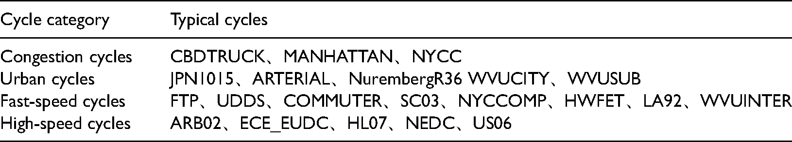
This paper selects 21 typical driving cycles as the basis for constructing comprehensive driving cycles, namely JPN1015, ARB02, ARTERIAL, CBDTRUCK, COMMUTER, ECE_EUDC, FTP, HL07, HWFET, LA92, MANHATTAN, NEDC, NYCC, NYCCOMP, NurembergR36, SC03, UDDS, US06, WVUCTIY, WVUINTER, WVUSUB. The constructed comprehensive driving cycle is used as simulation cycle for IRDC model and optimized EMS.

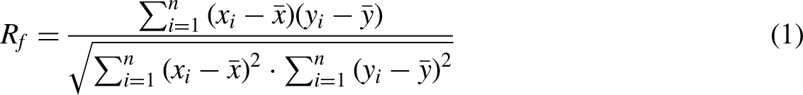
Generally, 10–18 characteristic parameters are selected for driving conditions (Montazeri-Gh et al., 2011; Wu et al., 2012). Twelve characteristic parameters were selected from four categories: time characteristic parameter, driving distance characteristic parameter, acceleration characteristic parameter and vehicle speed characteristic parameter, whose correlation coefficient metre $R_{r}$ can be calculated by formula (1). Four weakly related characteristic parameters of maximum vehicle speed, maximum acceleration, average acceleration, and average deceleration were obtained by principal component analysis (Guo and Wei, 2018).

R_{f} = \frac{\sum_{i = 1}^{n} (x_{i} - \bar{x}) (y_{i} - \bar{y})}{\sqrt{\sum_{i = 1}^{n} {(x_{i} - \bar{x})}^{2} \cdot \sum_{i = 1}^{n} {(y_{i} - \bar{y})}^{2}}}

(1)

where,

x_{i}

、

y_{i}

are the ith data of two sample data,

\bar{x}

、

\bar{y}

are the average of two sample data. If correlation coefficient of the characteristic parameter is between

0.2 \leq R_{r} \leq 0.4

, it is a weak correlation.

The above four characteristic parameters are selected to cluster 21 typical driving cycles, which are divided into congestion cycles, urban cycles, fast and high-speed cycles, as displayed in Table 1.

Table 1.

21 Typical working conditions.

Cycle category	Typical cycles
Congestion cycles	CBDTRUCK、MANHATTAN、NYCC
Urban cycles	JPN1015、ARTERIAL、NurembergR36 WVUCITY、WVUSUB
Fast-speed cycles	FTP、UDDS、COMMUTER、SC03、NYCCOMP、HWFET、LA92、WVUINTER
High-speed cycles	ARB02、ECE_EUDC、HL07、NEDC、US06

Connect five typical driving phases of NurembergR36 + HWFET + NYCC + US06 + UDDS to establish a comprehensive driving cycle, as shown in Figure 1.

Figure 1.

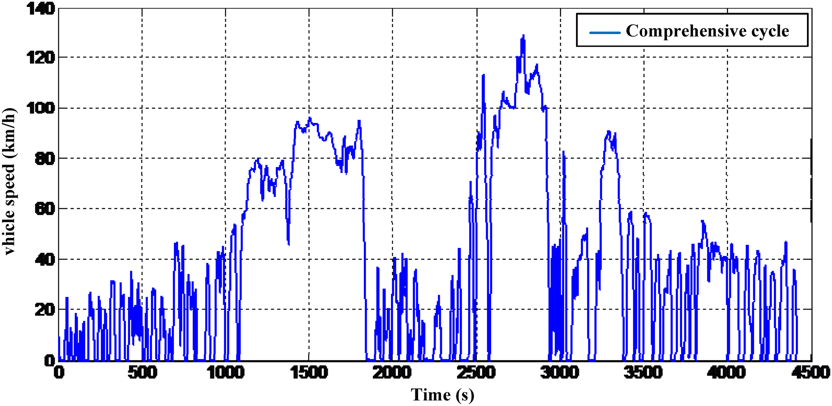
Comprehensive driving cycle.

Driving cycle identification model

The process of identifying driving cycles is described in Figure 2.

Figure 2.

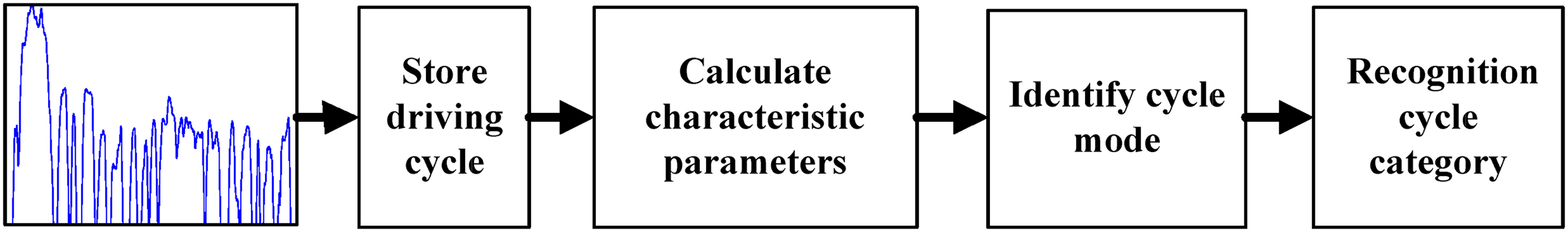
The process of identifying driving cycle.

At present, driving cycle recognition methods mainly include fuzzy logic, decision tree, support vector machine, BPNN and other methods (Zhang et al., 2014; Lecce and Calabrese, 2009). There are many driving cycles identification methods, but they can be basically divided into two categories: one is based on intelligent algorithm and the other is based on cluster analysis algorithm. Sun et al. (2017) used LVQ algorithm to identify four types of typical micro roads and three types of standard driving cycles, but more eigenvalues were selected, which increased the calculation time. Zhan et al. (2016) used the K-means clustering algorithm based on genetic optimization to construct the driving cycle identification model. However, this method has a large amount of calculation and low stability of identification rules. However, which of these two methods is most suitable for the actual driving cycle identification remains to be determined. Therefore, this paper establishes a driving cycle recognizer of K-means + and BPNN to analyses its recognition effect. The comprehensive driving cycle is divided at a time interval of 120 s, and then each sub-cycle area is identified separately (Zhang et al., 2020; Xie et al., 2018). The cycle identification results are represented by numbers 1, 2, 3 and 4, which represent congestion cycles, urban cycles, suburban cycles and high-speed cycles respectively.

BPNN driving cycle identification model

BPNN mainly includes three layers of neurons: input layer, hidden layer and output layer. Its topology is depicted in Figure 3. It can be seen that each node is connected by weights and thresholds, which rely on the forward propagation of signal and the backward propagation of error to adjust so as to achieve the desired output.

Figure 3.

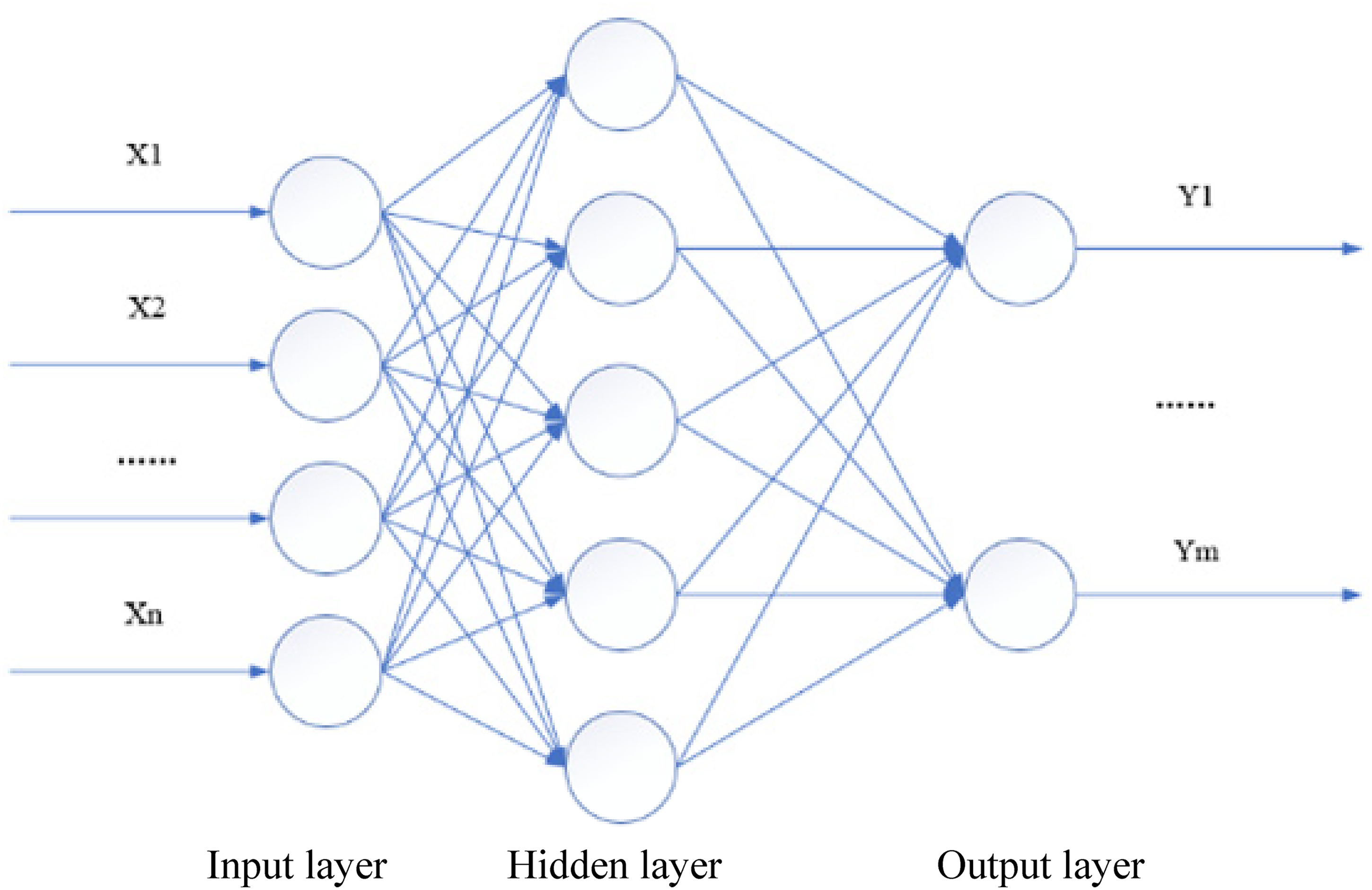
BPNN topology.

The BPNN driving cycle recognition model is constructed in MATLAB/Simulink, and the steps are described in Figure 4.

Figure 4.

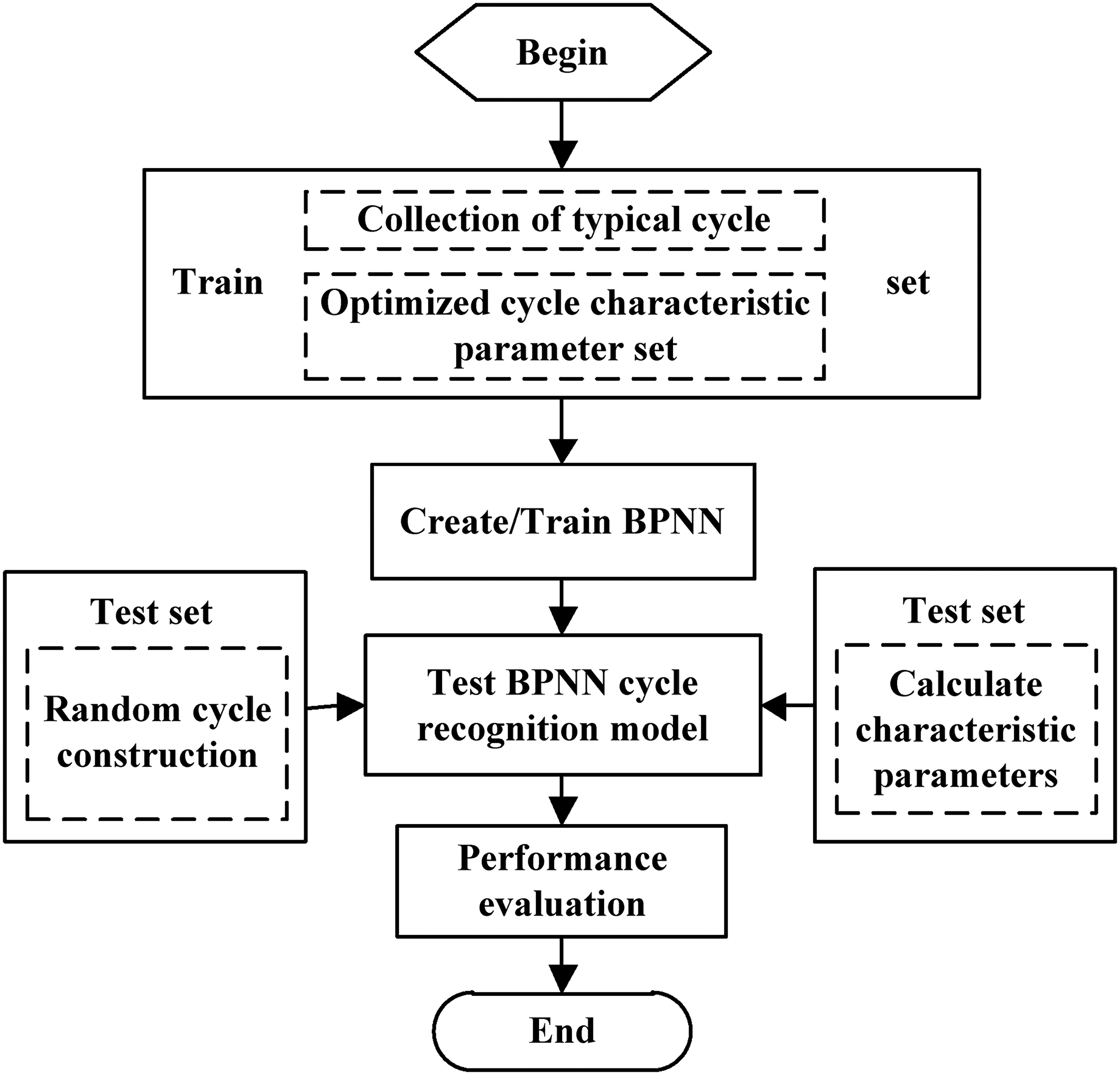
BPNN calculation process.

According to the BPNN working process, the newff statement is used to write the BPNN cycle recognition program by the MATLAB soft, and build the BPNN cycle recognition model in SIMULINK, as depicted in Figure 5.

Figure 5.

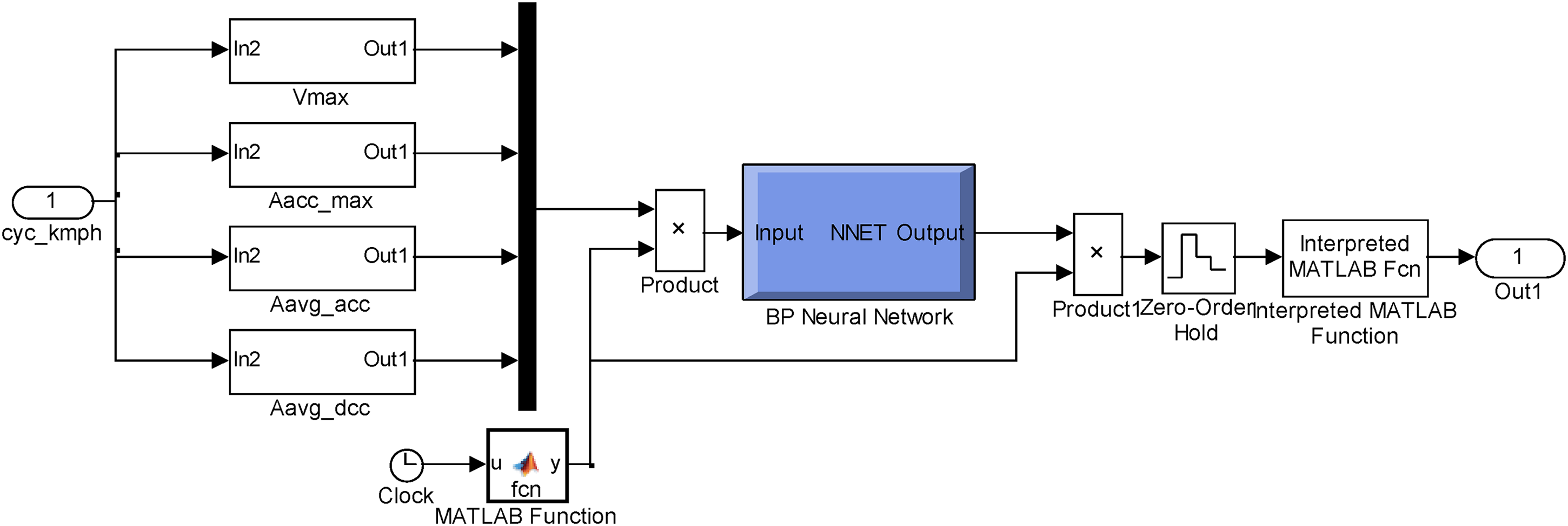
BPNN cycle recognition model.

Simulation and comparative analysis

The BPNN and K-means + cycle recognition results are compared with the desired output results, as be demonstrated in Figure 6. In order to visually analyse recognition effect of two methods, the difference between recognition results and the expected output results are calculated. Results of two recognition errors are delineated in Figure 7Fig. 7 and Figure 8Fig. 8. The more the difference is on the zero line, the better the recognition result is.

Figure 6.

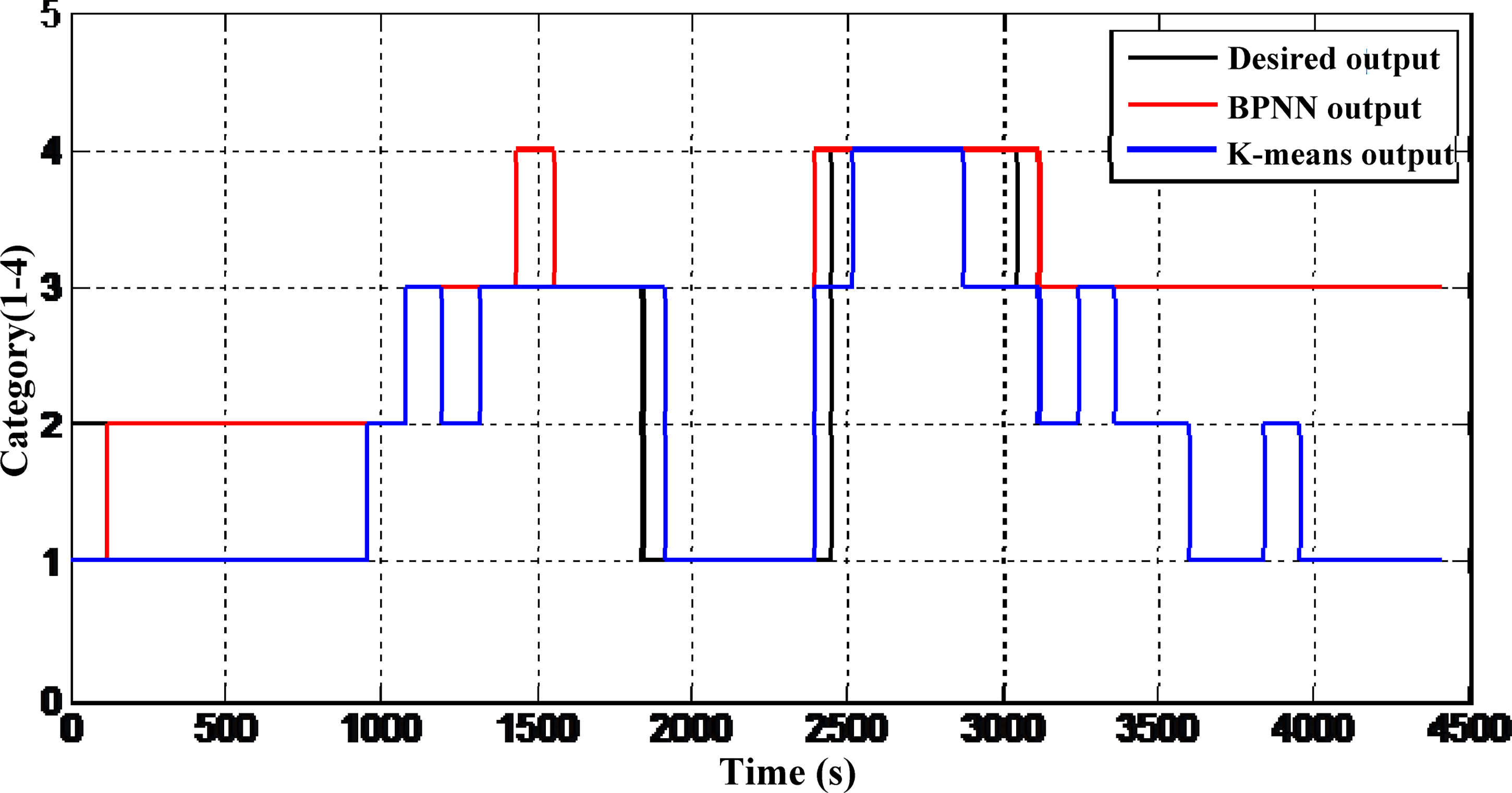
BPNN cycle recognition results.

Figure 7.

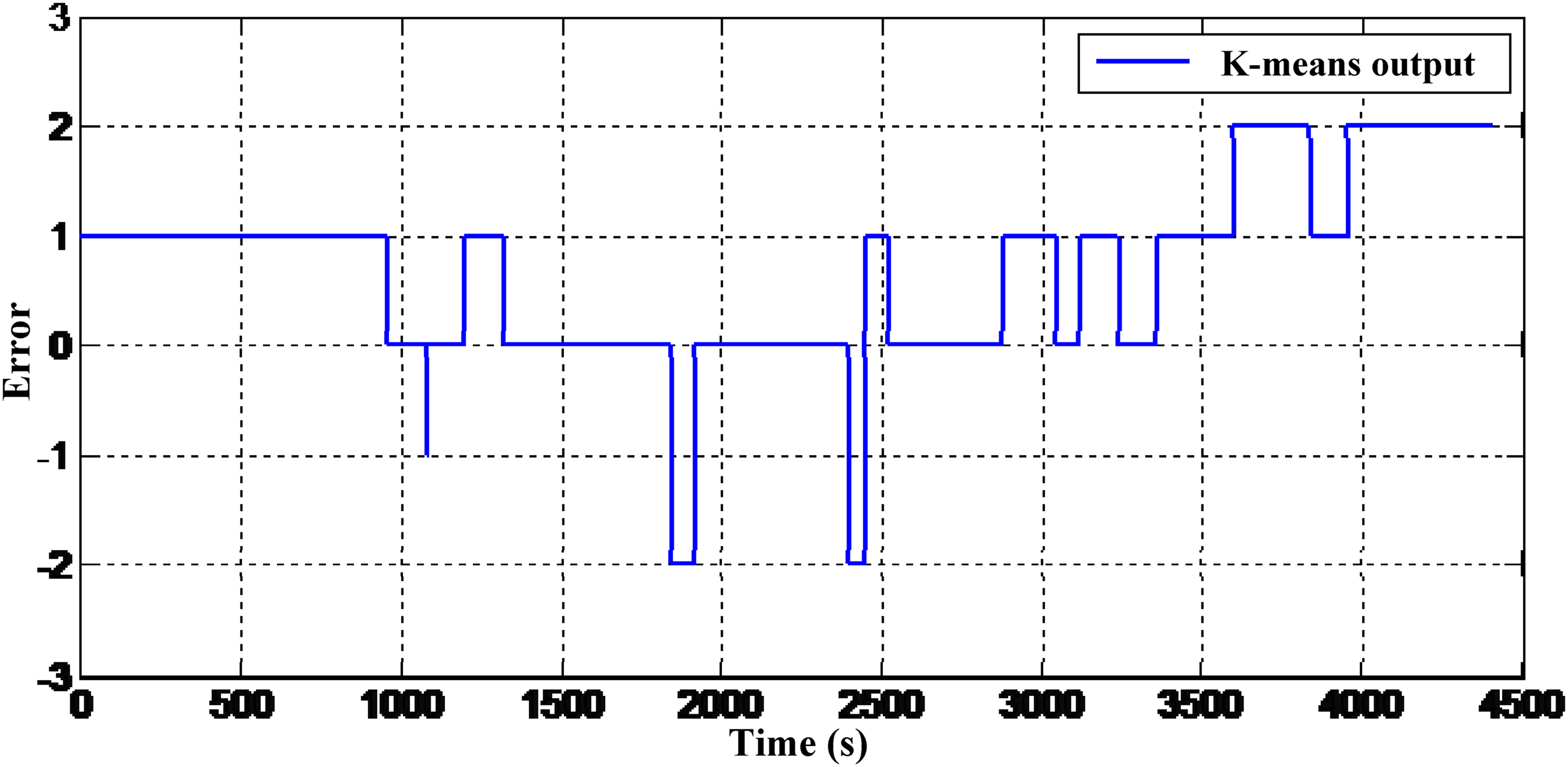
K-means + cycle recognition error results.

Figure 8.

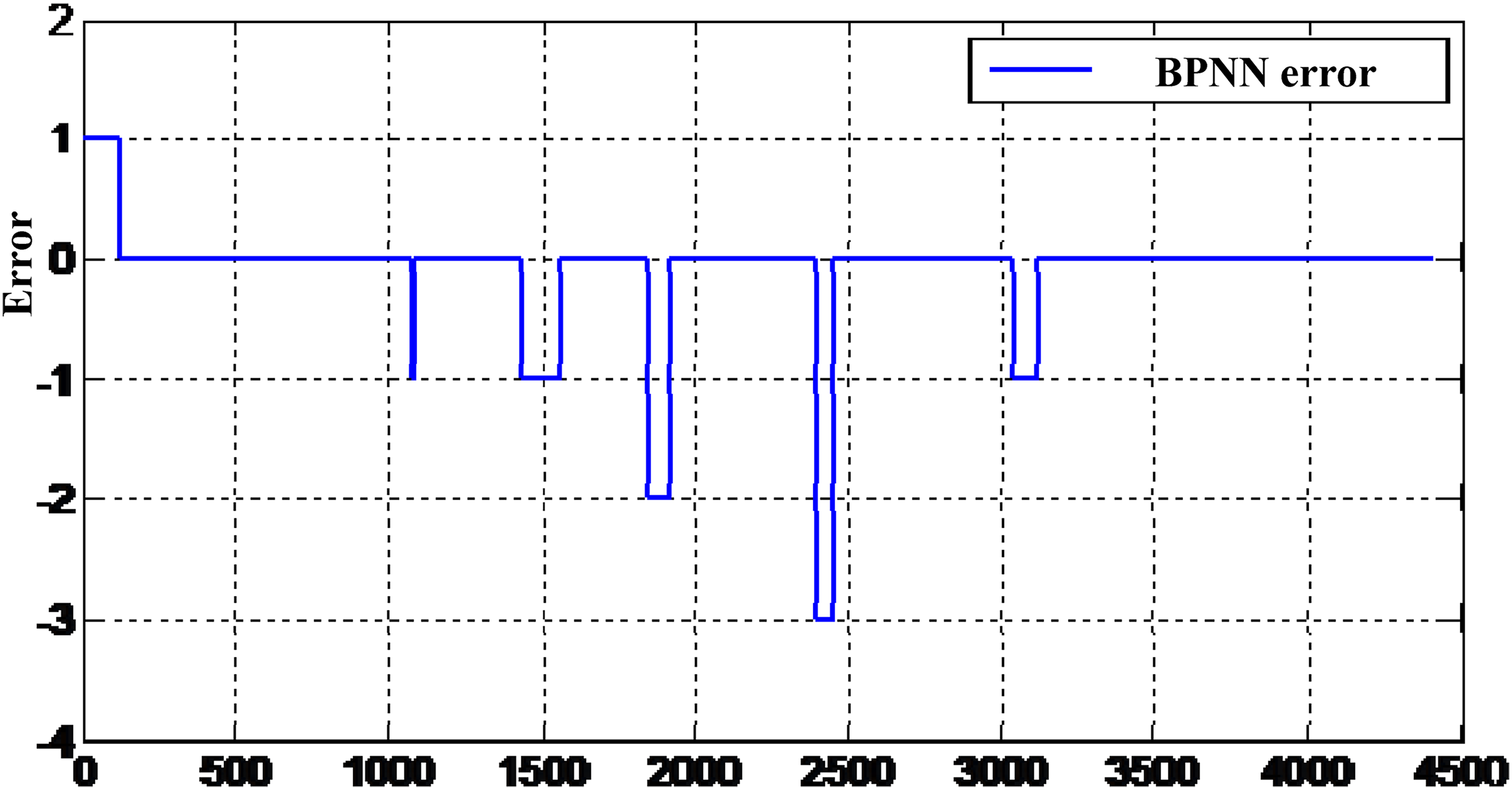
BPNN cycle recognition error results.

Through statistics, the accuracy of K-means + cycle recognition is 73%, and the accuracy of BPNN cycle recognition can reach 90.2%, which meets the needs of engineering use. Therefore, BPNN recognition model is adopted as the basis of energy management strategy design.

Design of A-EMS

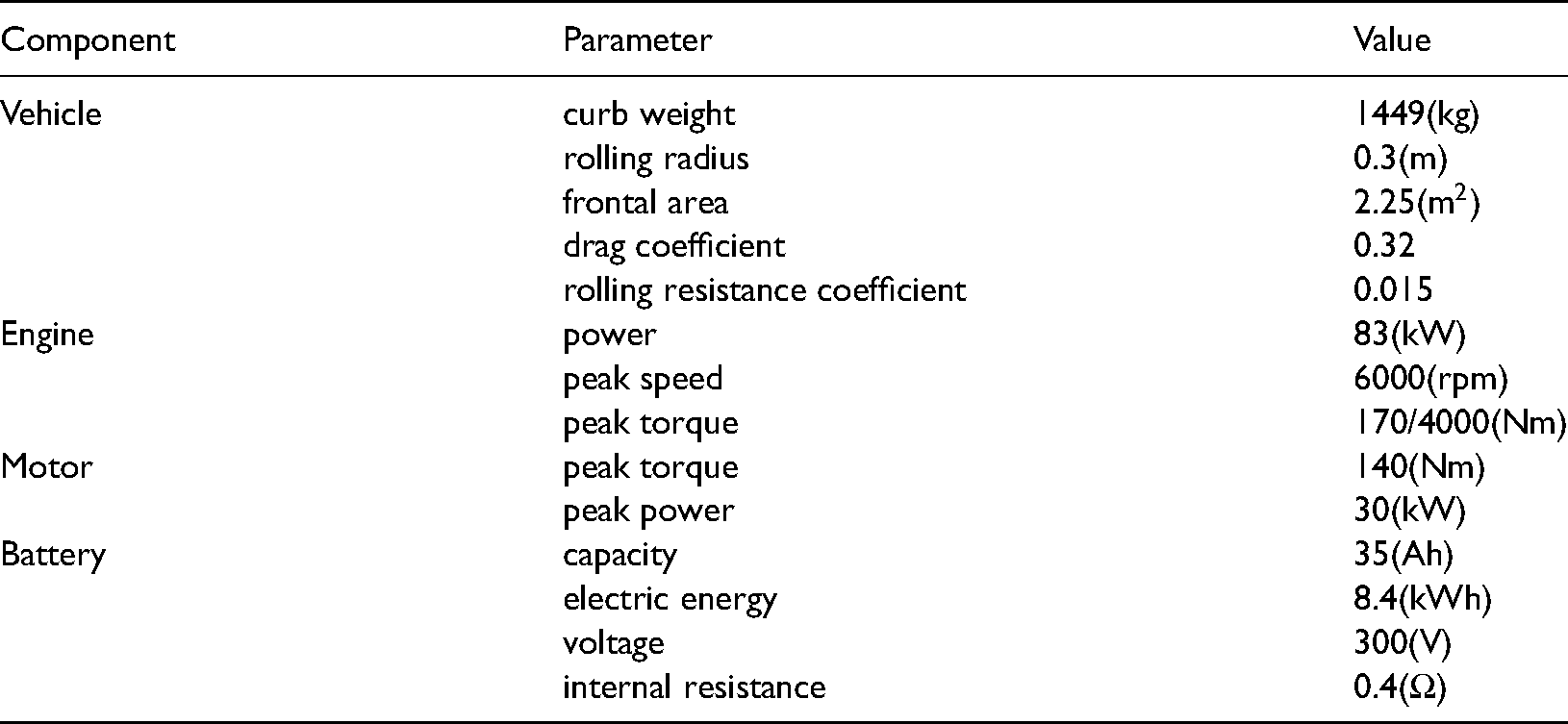
The configuration of PHEV can be divided into three types: serial, parallel and hybrid (Sorrentino et al., 2011). This paper takes the parallel PHEV with P2 configuration as research object, whose power system structure is shown in Figure 9. The motor is located between gearbox and engine, and is coaxially connected with engine, which can be used as motor or generator by connected to a lithium ion battery. Due to the mechanical connection between the engine and the wheel, the fuel economy of this configuration is greatly affected by the driving cycles, which is also a significant reason for carrying out the research on driving cycle identification. The parameters of vehicle and key components are displayed in Table 2.

Figure 9.

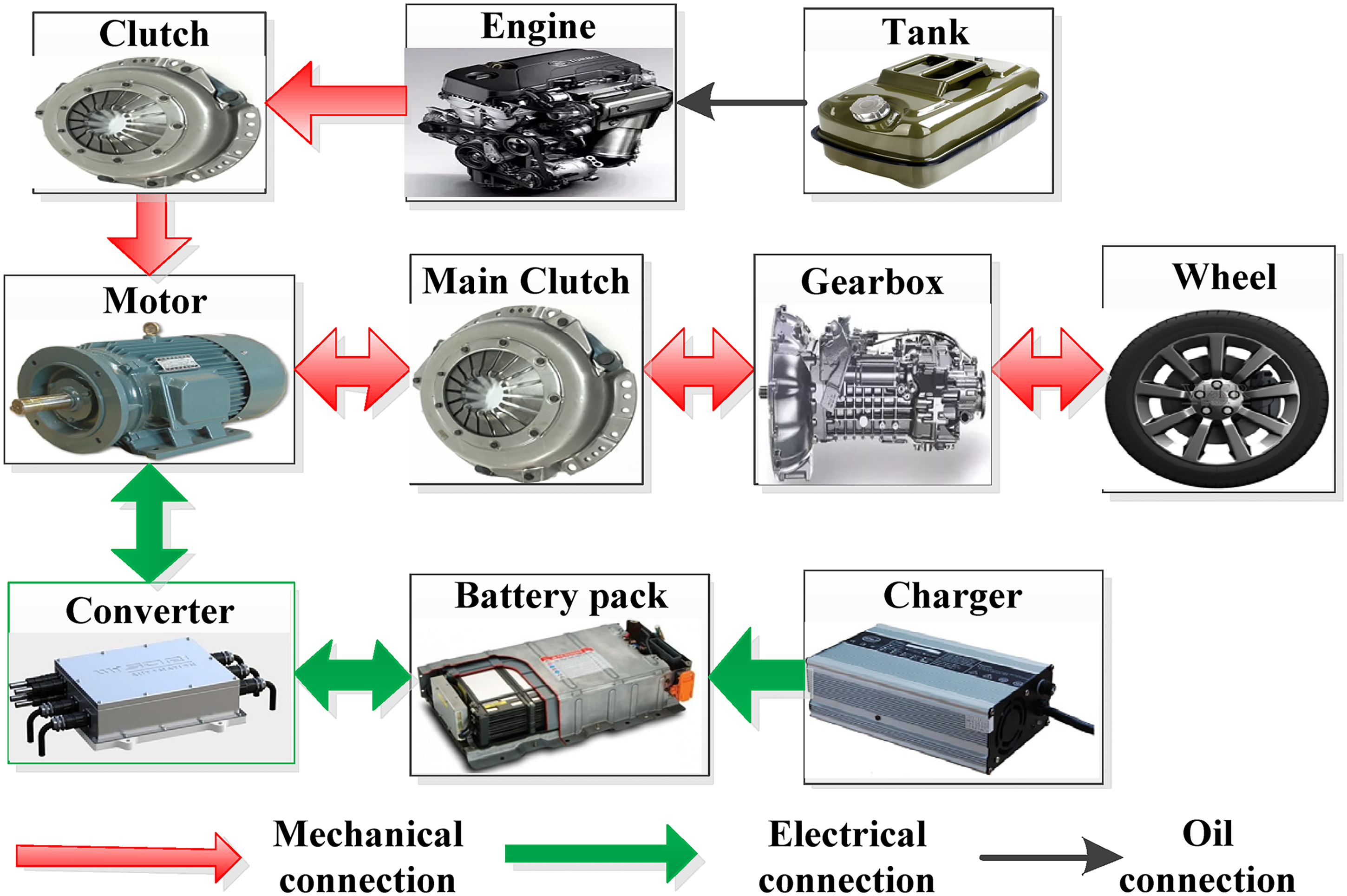
Structure of a parallel PHEV with P2 configuration.

Table 2.

PHEV parameters.

Component	Parameter	Value
Vehicle	curb weight	1449(kg)
	rolling radius	0.3(m)
	frontal area	2.25 $(m^{2})$
	drag coefficient	0.32
	rolling resistance coefficient	0.015
Engine	power	83(kW)
	peak speed	6000(rpm)
	peak torque	170/4000(Nm)
Motor	peak torque	140(Nm)
Motor	peak power	30(kW)
Battery	capacity	35(Ah)
	electric energy	8.4(kWh)
	voltage	300(V)
	internal resistance	0.4( $Ω$ )

Establishment and solution of optimal objective function

Establishment of optimal objective function

EMS optimization objectives are diverse, such as vehicle fuel consumption, exhaust emissions, operating costs, etc (Nuesch et al., 2014). This paper takes the minimum fuel consumption as the optimization objective J, power battery SOC as the state variable x, and motor output torque as the control variable u. The constraints are mainly engine and motor output torque and power range, as well as the voltage, current and power range of power battery (Kim et al., 2012). The expression of EMS optimization objectives is: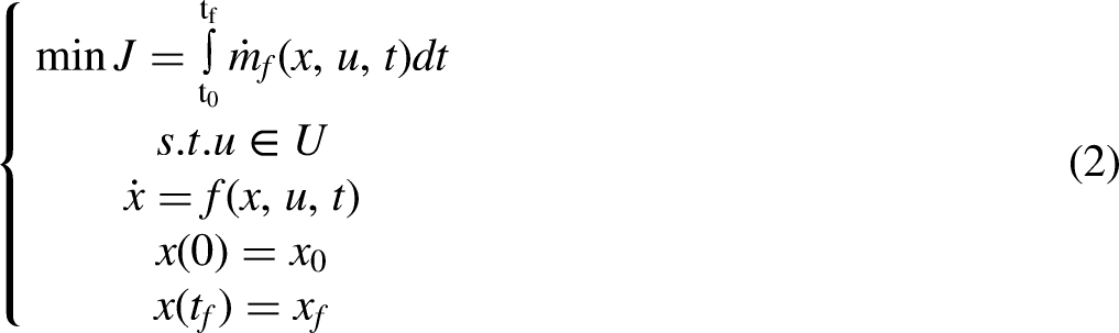

{\begin{matrix} min J = \int_{t_{0}}^{t_{f}} {\dot{m}}_{f} (x, u, t) d t \\ s . t . u \in U \\ \dot{x} = f (x, u, t) \\ x (0) = x_{0} \\ x (t_{f}) = x_{f} \end{matrix}

(2)

t_{0}

is the initial time,

t_{f}

is the end time,

{\dot{m}}_{f}

denotes the instantaneous fuel consumption rate of the engine, and U means the control domain.

Under the premise of ensuring the power performance of PHEV, whose power system is regarded as a complex nonlinear system, and the minimum fuel consumption problem is regarded as the optimal control problem with constraint.

Performance indicator function

Although PMP algorithm can achieve the optimization of exhaust emissions, battery life and other objectives, this paper only takes the minimum fuel consumption as the optimization objective of EMS. The performance index function is:

min_{T_{e}, n_{e} \in D} J = \int_{t_{0}}^{t_{f}} \dot{m} (u (t), t) d t

(3)

where

T_{e}

n_{e}

, D are the torque, speed and feasible region of engine,

u (t)

denotes the output torque of motor,

\dot{m} (u (t), t)

refers to the fuel consumption of the engine when the output torque of the motor is

u (t)

State variable

SOC is taken as the state variable of dynamical system, and its expression is as follows.

x (t) = S O C (t) = S O C (t_{0}) - \int_{t_{0}}^{t} \frac{I_{b} (τ)}{Q_{b}} d τ

(4)

where,

Q_{b}

is power battery capacity;

I_{b}

(τ) is the current of power battery at the τ moment.

According to PMP, the state transfer equation of power battery can be expressed as:

\overset{\cdot}{S O C (t)} {\begin{matrix} - \frac{V_{o c} (S O C) - \sqrt{V_{o c} {(S O C)}^{2} - 4 \cdot P_{b} (T_{m})} \cdot R_{o} (S O C)}{R_{o} (S O C) \cdot Q_{b}} . η_{b}, d i s c h a r g e \\ \frac{V_{o c} (S O C) - \sqrt{V_{o c} {(S O C)}^{2} - 4 \cdot P_{b} (T_{m}) \cdot R_{o} (S O C)}}{R_{o} (S O C) \cdot Q_{b} \cdot η_{b}}, c h a r g e \end{matrix}

(5)

where,

V_{o c}

R_{o}

η_{b}

and

P_{b}

are the open circuit voltage, equivalent internal resistance, charging-discharge efficiency and output power of power battery respectively.

Constraints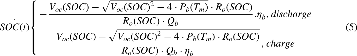

Considering the service life of power battery, the minimum available value of SOC is set as 0.4. In addition, the operating characteristics of the motor during driving and braking can be approximately regarded as symmetric. The global optimization objectives and constraints of EMS are described in equation (6).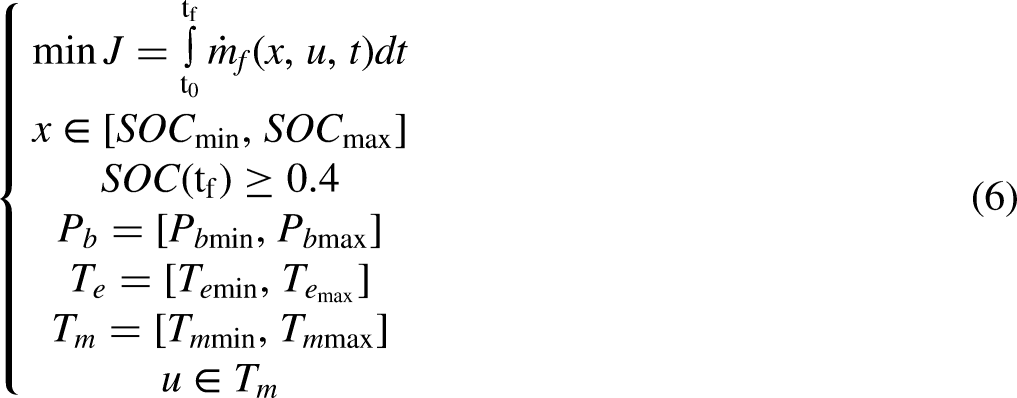

{\begin{matrix} min J = \int_{t_{0}}^{t_{f}} {\dot{m}}_{f} (x, u, t) d t \\ x \in [S O C_{\min}, S O C_{\max}] \\ S O C (t_{f}) \geq 0.4 \\ P_{b} = [P_{b \min}, P_{b \max}] \\ T_{e} = [T_{e \min}, T_{e_{\max}}] \\ T_{m} = [T_{m \min}, T_{m \max}] \\ u \in T_{m} \end{matrix}

(6)

Solution optimal objective function

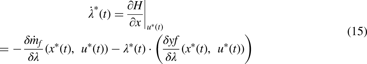
The global optimization problem can be transformed into several instantaneous optimization problems with Hamiltonian functions by introducing costate variable. Hamilton function can be expressed as equation (7), which is instantaneous fuel consumption of engine plus costate variable multiplied by instantaneous SOC change (Kim et al., 2011).

H (x (t), λ (t), u (t), t) = {\dot{m}}_{f} (x (t), u (t), t) + λ (t) \cdot f (x (t), u (t), t)

(7)

where,

{\dot{m}}_{f} (x (t), u (t), t)

refers to the instantaneous fuel consumption of engine; λ(t) is costate variable, which is related to the driving cycle.

f (x (t), u (t), t)

is system state transition equation, which is equal to the first derivative of SOC with respect to time, and can be written as equation (8).

f (x (t), u (t), t) = \dot{S O C}

(8)

equation (7) can also be expressed as:

H (x (t), λ (t), u (t), t) = \frac{P_{e} (t)}{η_{e} (t)} + λ (t) \cdot \frac{P_{b} (t)}{η_{b} (t)}

(9)

where,

P_{e} (t)

is output power of engine;

η_{e} (t)

denotes the efficiency of converting chemical energy into mechanical energy;

P_{b} (t)

and

η_{b} (t)

respectively represent output power and charge-discharge efficiency of power battery.

In order to solve the minimum value of Hamiltonian function at every moment, the optimal control law $u^{*} (t)$ can be obtained, which is expressed as:

\begin{matrix} u^{*} (t) = a r g min H (x (t), λ (t), u (t), t) \\ = a r g min H {{\dot{m}}_{f} (x (t), u (t), t) + λ (t) \cdot f (x (t), u (t), t)} \end{matrix}

(10)

Costate transition equation can be written as:

λ (\dot{t}) = - \frac{\partial H}{\partial x}

(11)

Corresponding to the optimal control law

u^{*} (t)

, state variables and costate variable should satisfy the following conditions:

x^{*} (t_{0}) = x_{0}

(12)

x^{*} (t_{f}) = x_{t a r g e t}

(13)

x (\dot{t}) = {\frac{\partial H}{\partial λ} |}_{u^{*} (t)} = f (x^{*} (t), u^{*} (t), t)

(14)

\begin{matrix} {\dot{λ}}^{*} (t) = {\frac{\partial H}{\partial x} |}_{u^{*} (t)} \\ = - \frac{δ {\dot{m}}_{f}}{δ λ} (x^{*} (t), u^{*} (t)) - λ^{*} (t) \cdot (\frac{δ y f}{δ λ} (x^{*} (t), u^{*} (t))) \end{matrix}

(15)

where

x^{*} (t_{0})

is the initial state of state variable;

x^{*} (t_{f})

means state variable terminates;

x_{t a r g e t}

represents the target state during termination phase of state variable.

Design of ECMS

In 1999, Paganelli et al. proposed an ECMS based on the PMP semi-analytical method, which has the characteristics of small amount of calculation, strong real-time performance, and wide application range (Tulpule et al., 2010). The objective function of ECMS uses numerical methods to solve the control law that minimizes the equivalent fuel consumption in the feasible region, which is the output of power system. Figure 10 depicts the working process of ECMS, which calculates demand torque in real time through pedal opening, generates all engine and motor control law combinations within the feasible region, and then calculates the equivalent fuel consumption of all combinations according to the working efficiency characteristic diagram engine and motor. The optimal power distribution of power system is the combination of control law that make engine work in the high efficiency area and minimize the objective function.

Figure 10.

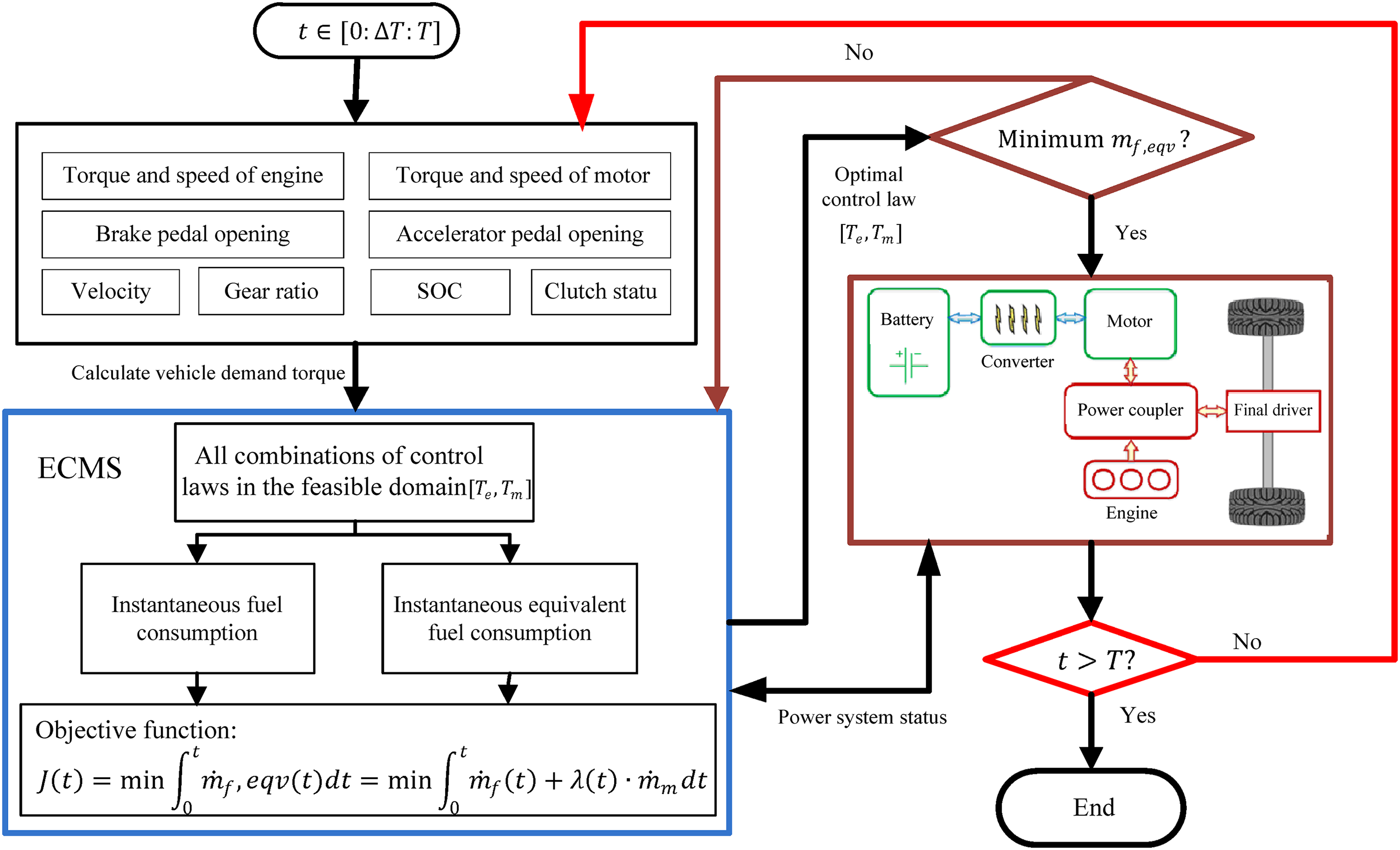
Working process of ECMS.

Calculation of EF and establishment of EF map diagram

EF determines power output ratio of engine and motor in A-ECMS strategy, whose working process is as follows. Firstly, the initial SOC and mileage are obtained; Secondly, the off-line optimal control method and GA were employed to solve the initial value of costate, and EF MAP was established under the conditions of different initial SOC and mileage. Then, EF under actual driving conditions can be obtained by interpolating in EF MAP, and be modified by current velocity and SOC. Finally, power output of engine and motor is allocated by EF, which reduces fuel consumption of vehicle.

Calculation of EF

EF is usually solved by iterative search method, which requires a lot of iteration and calculation, increasing the calculation time. In order to solve the problem, GA is adopted to obtain the initial value of EF, which takes the objective function value as the search information, so as to get appropriate EF. The GA working process for solving EF is described in Figure 11. GA, proposed by John Holland, mainly includes three genetic operators: selection, crossover and mutation. GA can optimize the evolution mechanism of organisms through random search iteration, and has the advantages of good robustness and high efficiency for solving optimization problems of nonlinear systems (Khayyam and Bab-Hadiashar, 2014). Because monomer genetic operators operate in the state of random disturbance, the optimal solution to solve the population is monomer to random migration. Compared with traditional random search methods, genetic random search operation is an efficient and directed search. Therefore, an initial population is selected, then the objective function is calculated, and the fitness function is finally obtained by using Simulink and Cruise co-simulation. If the stop rule is satisfied, the optimal result is output; otherwise, the fitness evaluation of the generated population is conducted again, and after a certain number of iterations, until the stop rule is satisfied (Poursamad and Montazeri, 2008).

Figure 11.

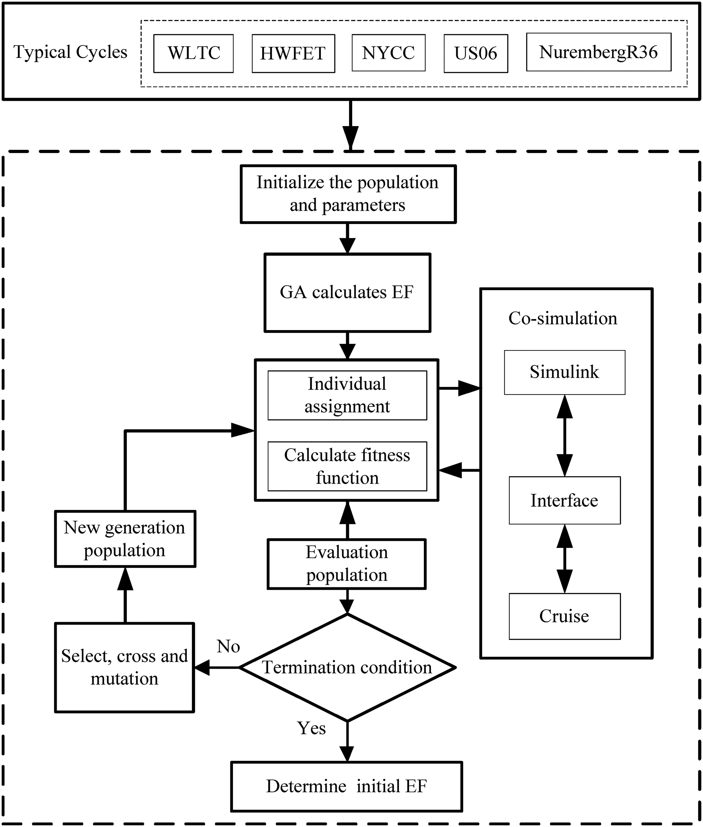
Equivalent factor calculation process.

Establishment of EF map diagram

Since the calculation of EF requires a large amount of calculation power, EF Map Diagram needs to be calculated offline under different cycles, so as to ensure the real-time and effectiveness of EMS.

When GA is used to calculate EF, the individual fitness function is expressed as:

f (λ) = min \int_{t_{0}}^{t_{f}} {\dot{m}}_{f} (u (t)) d t

(16)

Since initial SOC and driving range have a great influence on EF, in the process of establishing EF MAP Diagram, different initial SOC and driving range are selected to carry out multiple groups of simulation to calculate EF. The 1*, 2*, 3*, 4* and 5* WLTC cycles were selected, and the initial SOC was set to 0.4, 0.5, 0.6, 0.7, 0.8 and 0.9 respectively. Therefore, a total of 30 kinds of EF under initial conditions needed to be calculated.

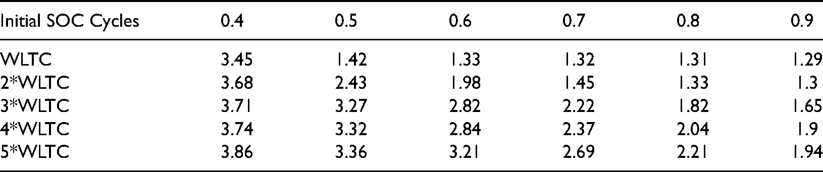
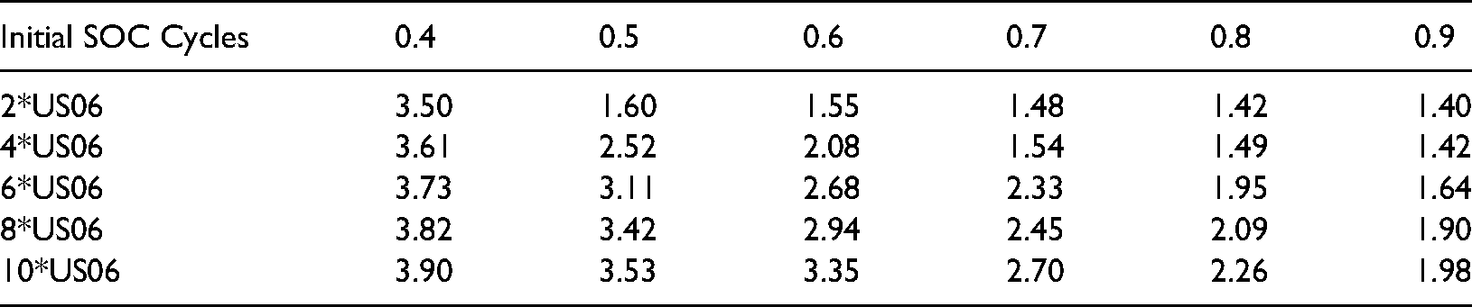
Taking 5 × WLTC cycle with initial SOC 0.9 as an example, the process of GA solving EF is illustrated. In order to improve the solving speed, the approximate range of solving EF is set as [1,4] and the maximum number of genetic iterations is set as 15. Then the GA function is called and a program is written to calculate the EF that makes the fitness function minimum, which is −1.94kg. Figure 12 depicts how the fitness function changes. Under 30 initial conditions, the solved EF is listed in Table 3.

Figure 12.

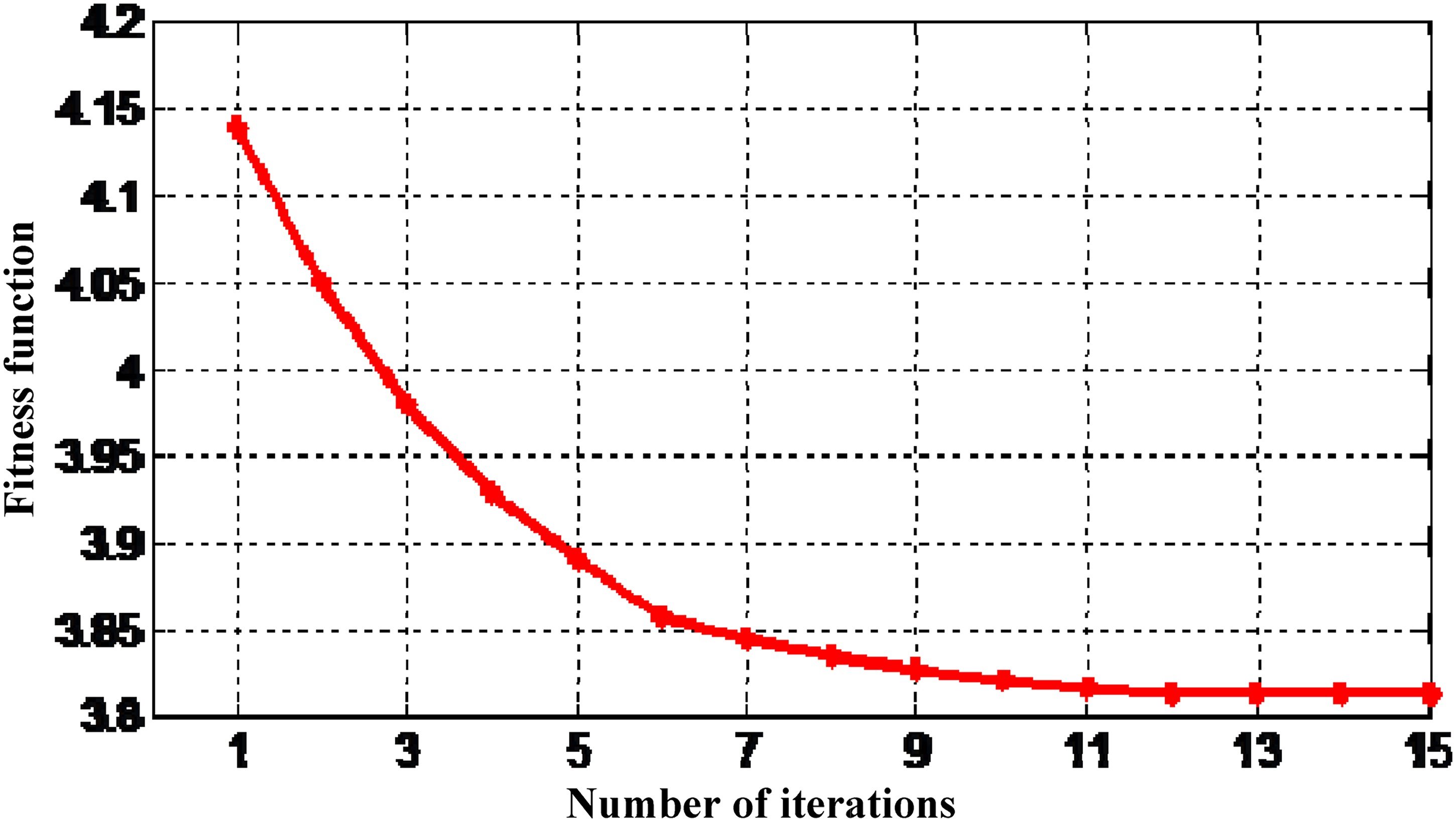
Variation of fitness function with iteration number.

Table 3.

EF obtained under WLTC cycles (unit: −1 × kg).

Initial SOC Cycles	0.4	0.5	0.6	0.7	0.8	0.9
WLTC	3.45	1.42	1.33	1.32	1.31	1.29
2*WLTC	3.68	2.43	1.98	1.45	1.33	1.3
3*WLTC	3.71	3.27	2.82	2.22	1.82	1.65
4*WLTC	3.74	3.32	2.84	2.37	2.04	1.9
5*WLTC	3.86	3.36	3.21	2.69	2.21	1.94

Initial SOC, mileage and EF are taken as the X-axis, Y-axis and Z-axis of EF MAP Diagram respectively, which is plotted according to the data in Table 3, and is shown in Figure 13.

Figure 13.

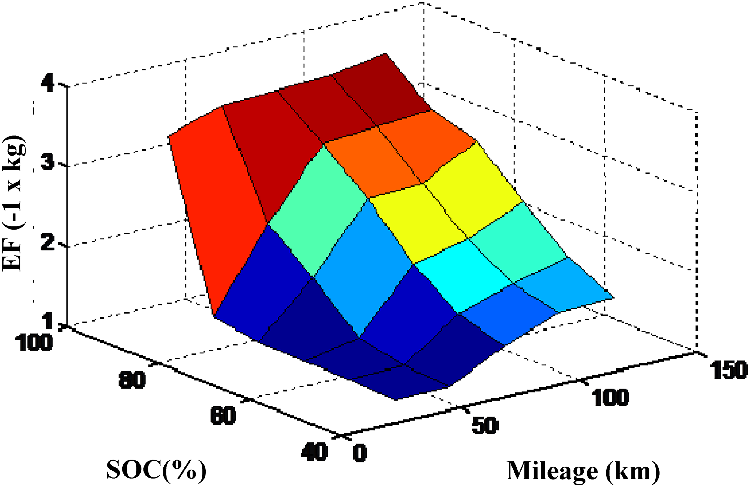
EF Map diagram changing with initial SOC and driving distance under WLTC cycles.

As can be seen from Figure 13, EF increases with the decrease of SOC, indicating that when SOC is insufficient, EF will increase. At this time, power system will increase working time of engine and prefer to use fuel, while working time of motor will decrease to ensure the stability of SOC. Under the same initial SOC, with the increase of Mileage, the EF will continue to increase, the power system will reduce the use of motor, increase working frequency of engine, delay the consumption of electric energy, so that SOC is at the minimum available value at the end of trip. If driving range is less than the pure electric range, the EF will not fluctuate much, and the power system mainly uses motor.

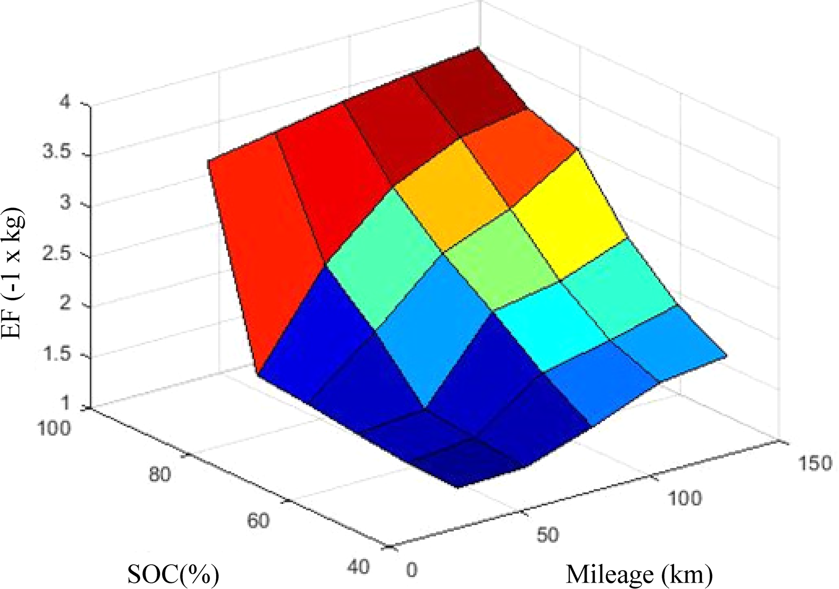
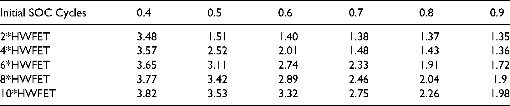
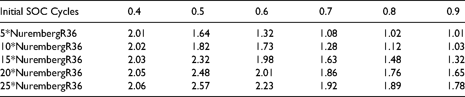
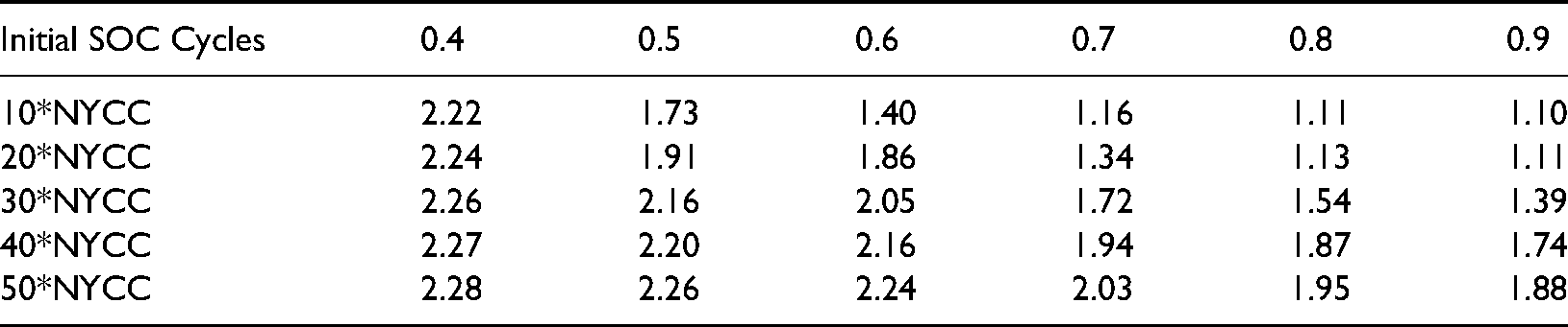
Repeat the above steps to solve the EF under HWFET, NurembergR36, NYCC and US06 cycle conditions respectively and established EF MAP diagram, so that the EF can be quickly obtained offline, which lays the foundation for A-ECSM strategy. Under four typical cycles, calculated EF data are listed in Table 4, Table 5, Table 6 and Table 7 respectively, and established EF MAP diagram is portrayed in Figure 14, Figure 15, Figure 16 and Figure 17respectively.

Figure 14.

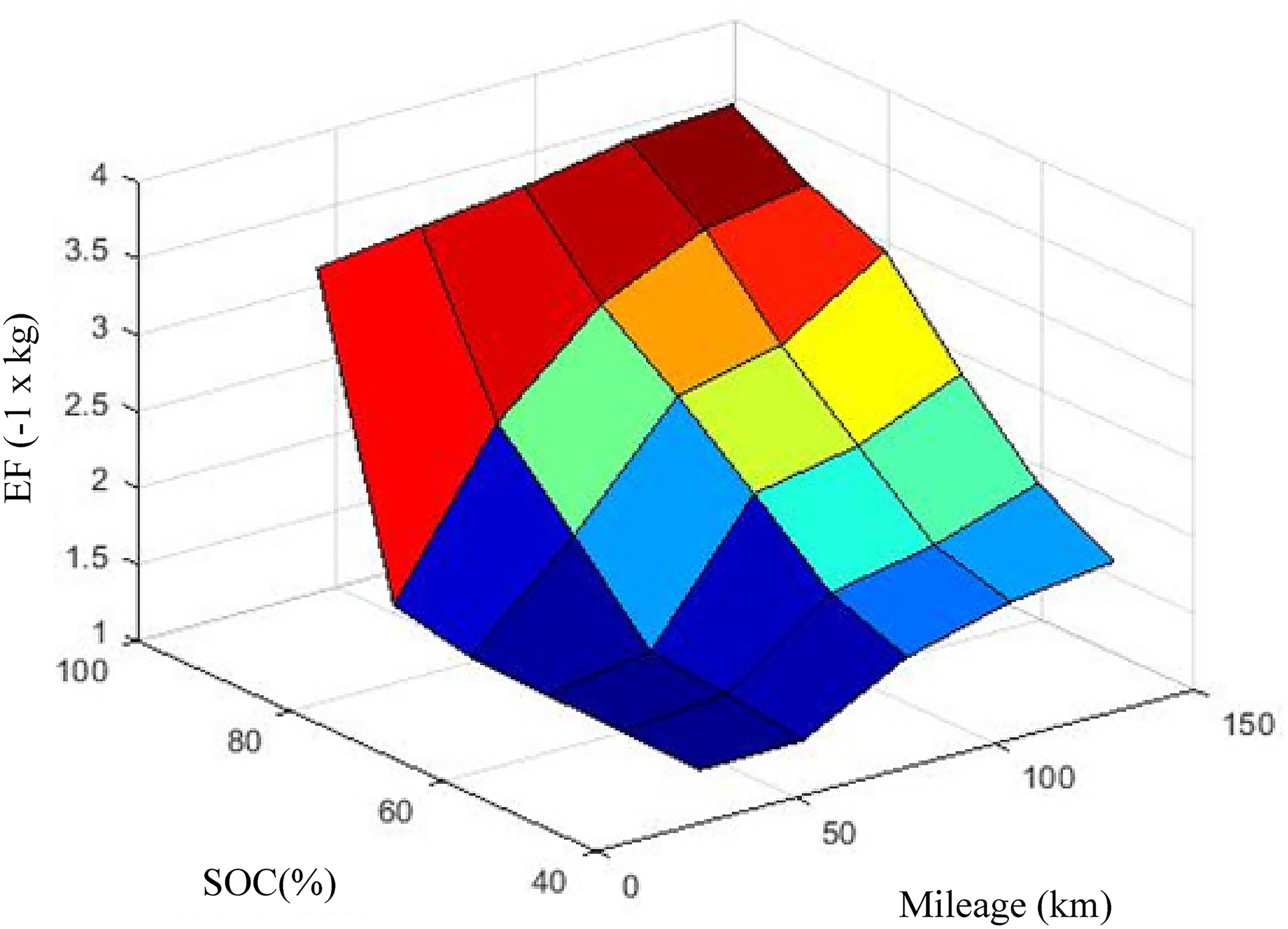
EF Map diagram established under HWFET cycles.

Figure 15.

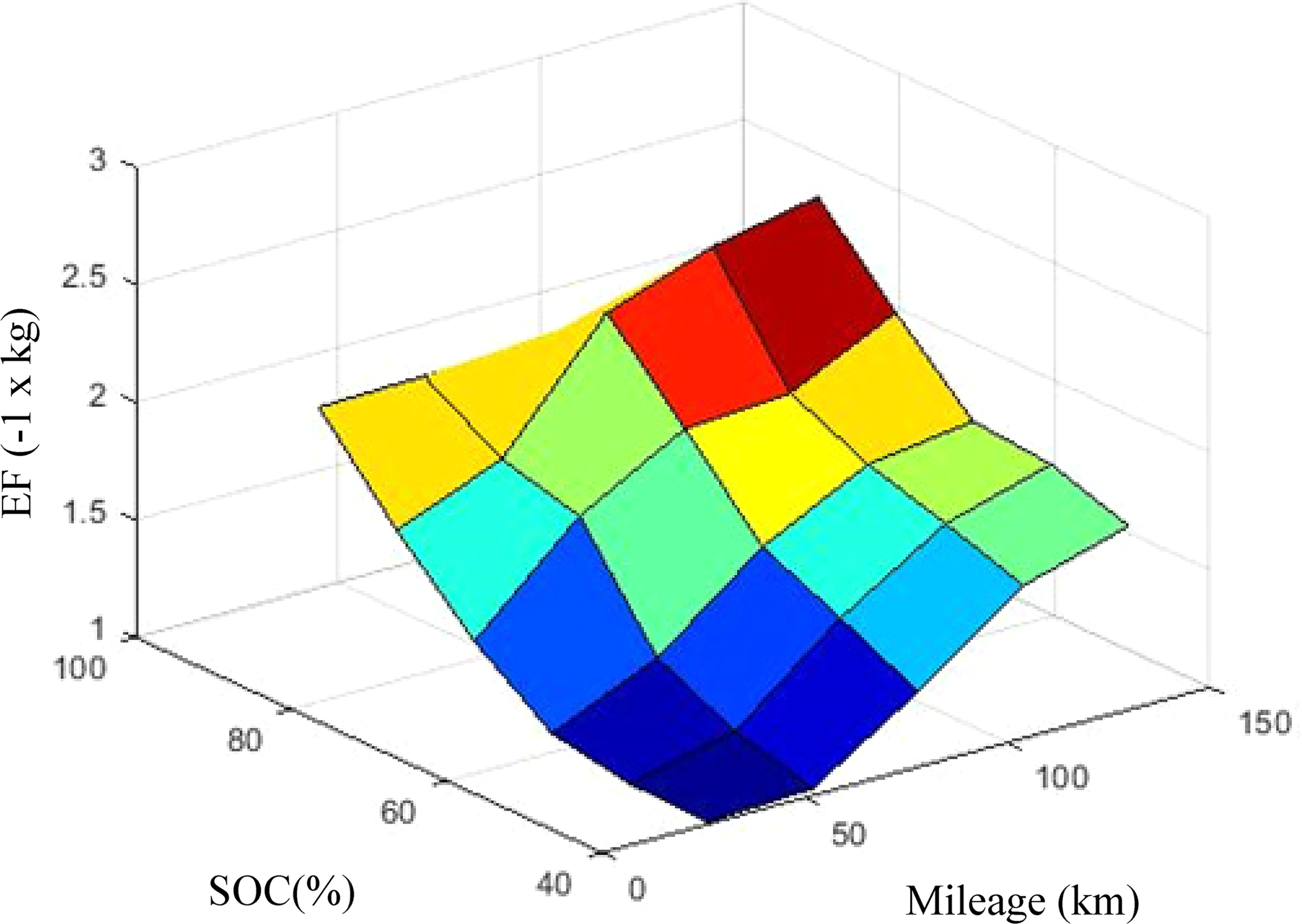
EF Map diagram established under NurembergR36 cycles.

Figure 16.

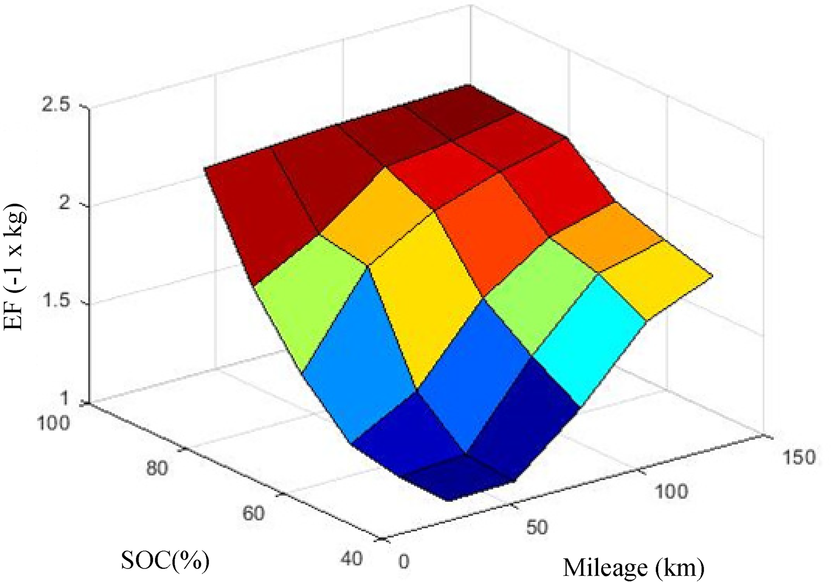
EF Map diagram established under NYCC cycles.

Figure 17.

EF Map diagram established under US06 cycles.

Table 4.

EF obtained under HWFET cycles (unit: −1 × kg).

Initial SOC Cycles	0.4	0.5	0.6	0.7	0.8	0.9
2*HWFET	3.48	1.51	1.40	1.38	1.37	1.35
4*HWFET	3.57	2.52	2.01	1.48	1.43	1.36
6*HWFET	3.65	3.11	2.74	2.33	1.91	1.72
8*HWFET	3.77	3.42	2.89	2.46	2.04	1.9
10*HWFET	3.82	3.53	3.32	2.75	2.26	1.98

Table 5.

EF obtained under NurembergR36 cycles (unit: −1 × kg).

Initial SOC Cycles	0.4	0.5	0.6	0.7	0.8	0.9
5*NurembergR36	2.01	1.64	1.32	1.08	1.02	1.01
10*NurembergR36	2.02	1.82	1.73	1.28	1.12	1.03
15*NurembergR36	2.03	2.32	1.98	1.63	1.48	1.32
20*NurembergR36	2.05	2.48	2.01	1.86	1.76	1.65
25*NurembergR36	2.06	2.57	2.23	1.92	1.89	1.78

Table 6.

EF obtained under NYCC cycles (unit: −1 × kg).

Initial SOC Cycles	0.4	0.5	0.6	0.7	0.8	0.9
10*NYCC	2.22	1.73	1.40	1.16	1.11	1.10
20*NYCC	2.24	1.91	1.86	1.34	1.13	1.11
30*NYCC	2.26	2.16	2.05	1.72	1.54	1.39
40*NYCC	2.27	2.20	2.16	1.94	1.87	1.74
50*NYCC	2.28	2.26	2.24	2.03	1.95	1.88

Table 7.

EF obtained under US06 cycles (unit: −1 × kg).

Initial SOC Cycles	0.4	0.5	0.6	0.7	0.8	0.9
2*US06	3.50	1.60	1.55	1.48	1.42	1.40
4*US06	3.61	2.52	2.08	1.54	1.49	1.42
6*US06	3.73	3.11	2.68	2.33	1.95	1.64
8*US06	3.82	3.42	2.94	2.45	2.09	1.90
10*US06	3.90	3.53	3.35	2.70	2.26	1.98

Design and establishment of A-ECMS

Design of A-ECMS

Due to large capacity of power battery and wide range of SOC changes, the full use of power battery power is the key to reducing fuel consumption of PHEV. In this paper, the deviation between SOC and reference SOC is used for feedback adjustment, so that SOC just drops to the minimum available value at the end of the trip.

In order for SOC to vary with reference SOC, average velocity and initial EF need to be considered. The modified expression of EF is:

λ (t) = λ_{0} + s (Δ S O C, t) + s (Δ V, t)

(17)

where,

λ_{0}

is initial EF,

s (Δ S O C, t)

means the SOC penalty factor, and

s (Δ V, t)

represents velocity penalty factor.

$λ (t)$ determines the ratio of torque distribution between engine and motor. If $λ (t)$ is larger, PHEV will use engine more frequently, and vice versa. Therefore, this parameter can be employed to adjust the ratio of engine and motor to operate .

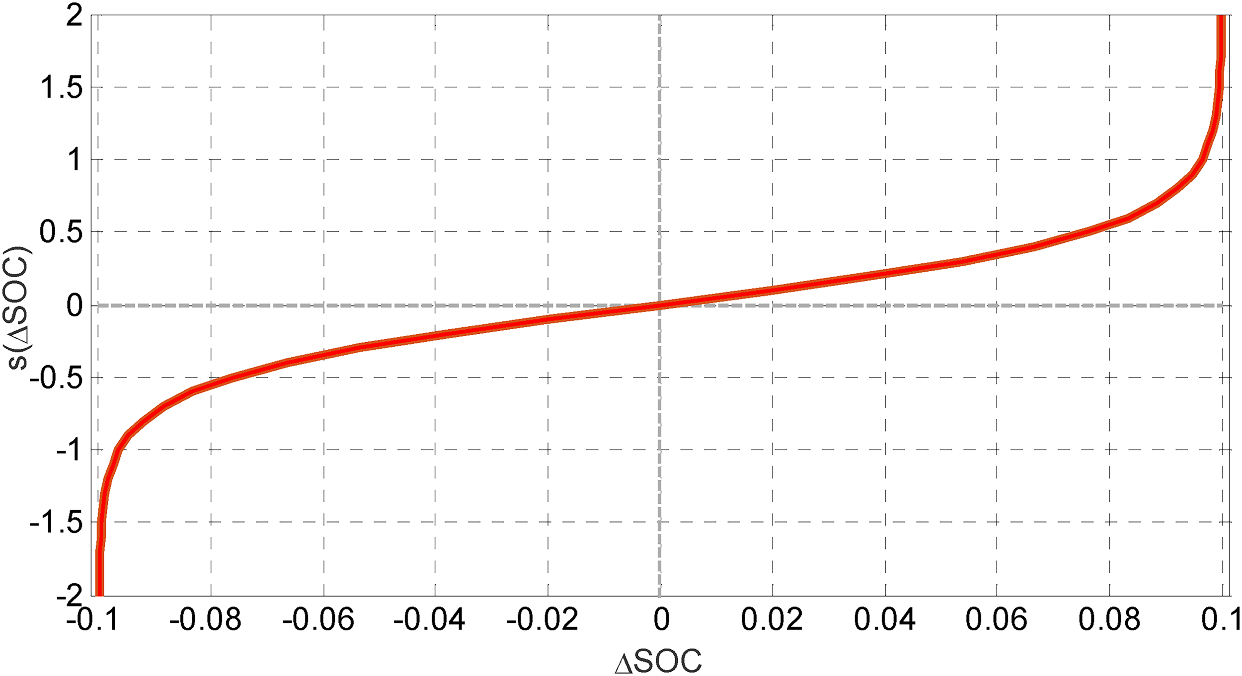
SOC penalty factor

In actual driving event, SOC will not follow completely with reference SOC. For example, as be displayed in Figure 18, when mileage is

S_{1}

and

Δ S O C > 0

, which indicates that actual SOC value is small, and the use of motor needs to be reduced. In this way,

λ (t)

needs to be increased to bias power system to use engine.

Figure 18.

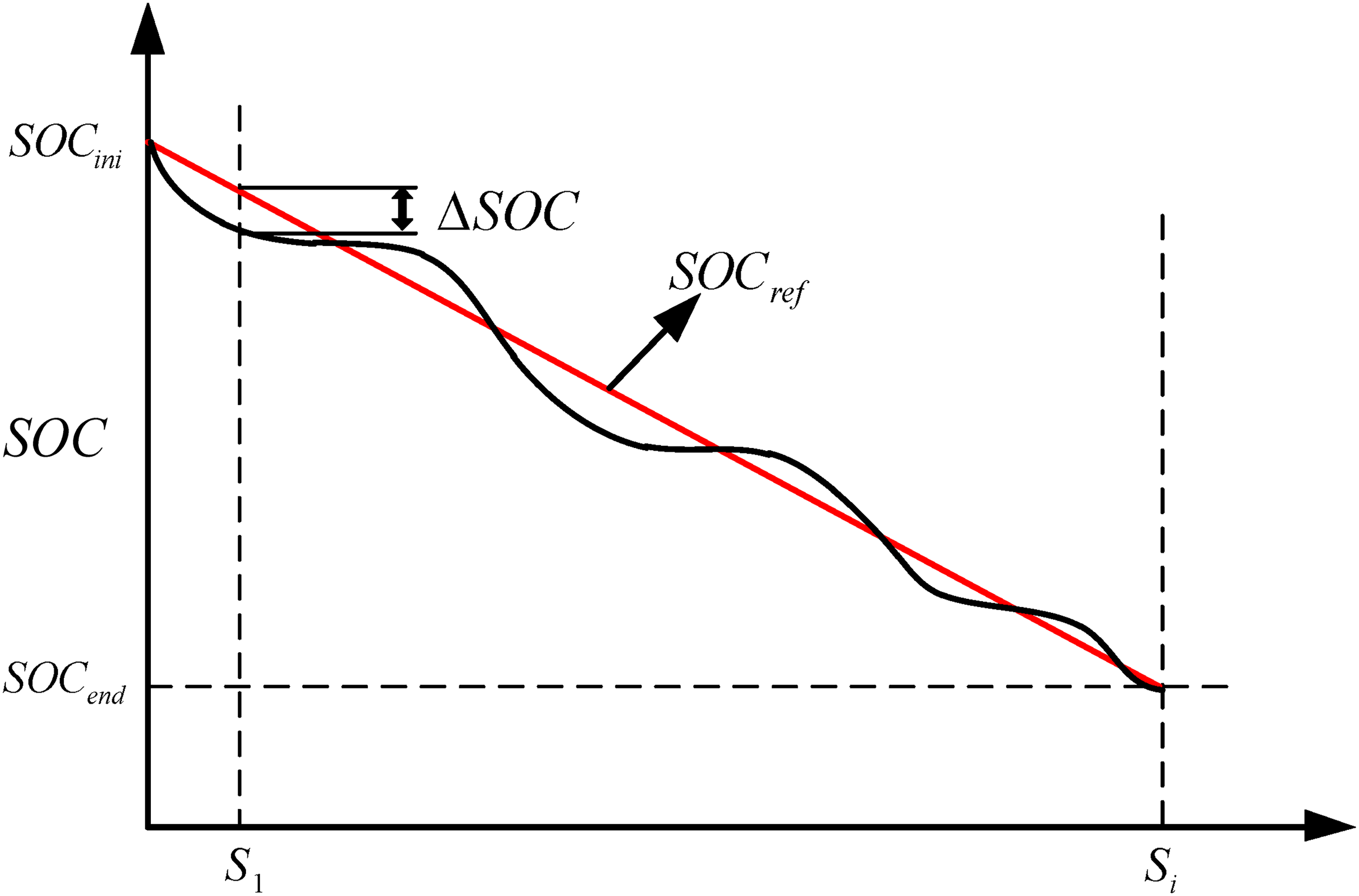
SOC and reference SOC change curve.

If the SOC deviates greatly from reference SOC, SOC penalty factor $s (Δ S O C, t)$ should be increased quickly, and vice versa. When $Δ S O C = S O C - S O C_{r e f} > 0$ , $s (Δ S O C, t)$ takes a positive value to increase power consumption, and vice versa. The expression of $s (Δ S O C, t)$ is as follows:

s (Δ SOC, t) = 0.25 \ln \frac{0.1 + Δ SOC}{0.1 - Δ SOC}

(18)

Taking range of

Δ S O C

as (−0.1, 0.1), variation curve of

s (Δ S O C, t)

with

Δ S O C

is shown in Figure 19. When SOC is much smaller than reference SOC,

s (Δ S O C, t)

decreases rapidly, and vice versa. Therefore,

s (Δ S O C, t)

can ensure that SOC decreases with reference SOC, so as to improve fuel economy.

Velocity penalty factor

Figure 19.

$s (Δ S O C, t)$ change curve with ΔSOC.

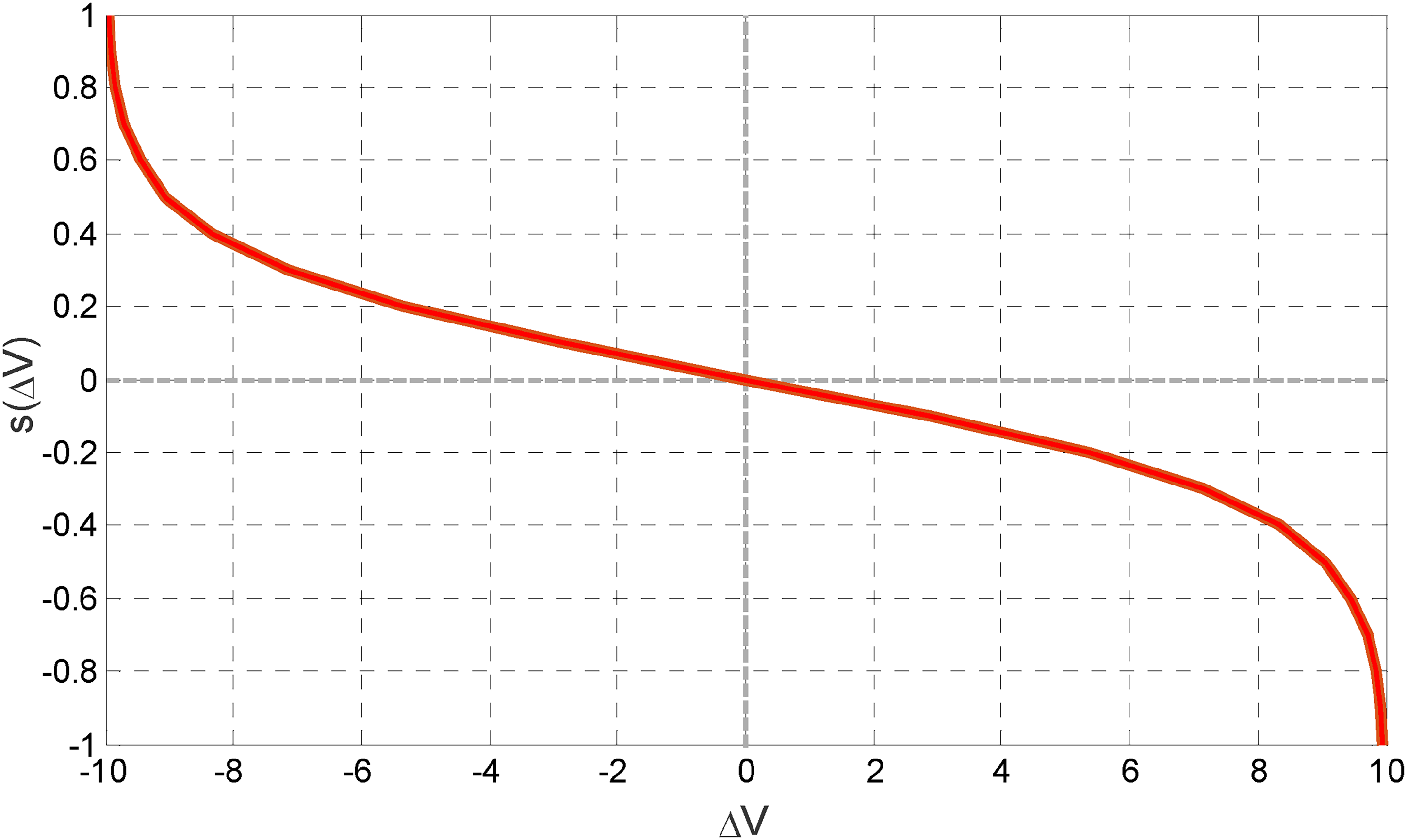
If velocity deviates greatly from average velocity, velocity penalty factor $s (Δ V, t)$ should increase rapidly, and vice versa. When $Δ V > 0$ , $s (Δ V, t)$ is positive to increase the power consumption, and vice versa. Therefore, $s (Δ V, t)$ can be written as:

s (Δ V, t) = \frac{1}{6} \ln \frac{10 + Δ V}{10 - Δ V}

(19)

Taking range of

Δ V

as (−10, 10), variation curve of

s (Δ V, t)

with

Δ V

is depicted in Figure 20.

Figure 20.

$s (Δ V, t)$ change curve with ΔSOC.

Establishment of A-ECMS

A-ECMS can apply real-time adjustment of EF to solve the optimal control function, which is employed to update the future driving state, so that updated EF can be used to solve the minimum function of equivalent fuel consumption, and finally reduce the error caused by the high sensitivity of EF. The working process is portrayed in Figure 21.

Figure 21.

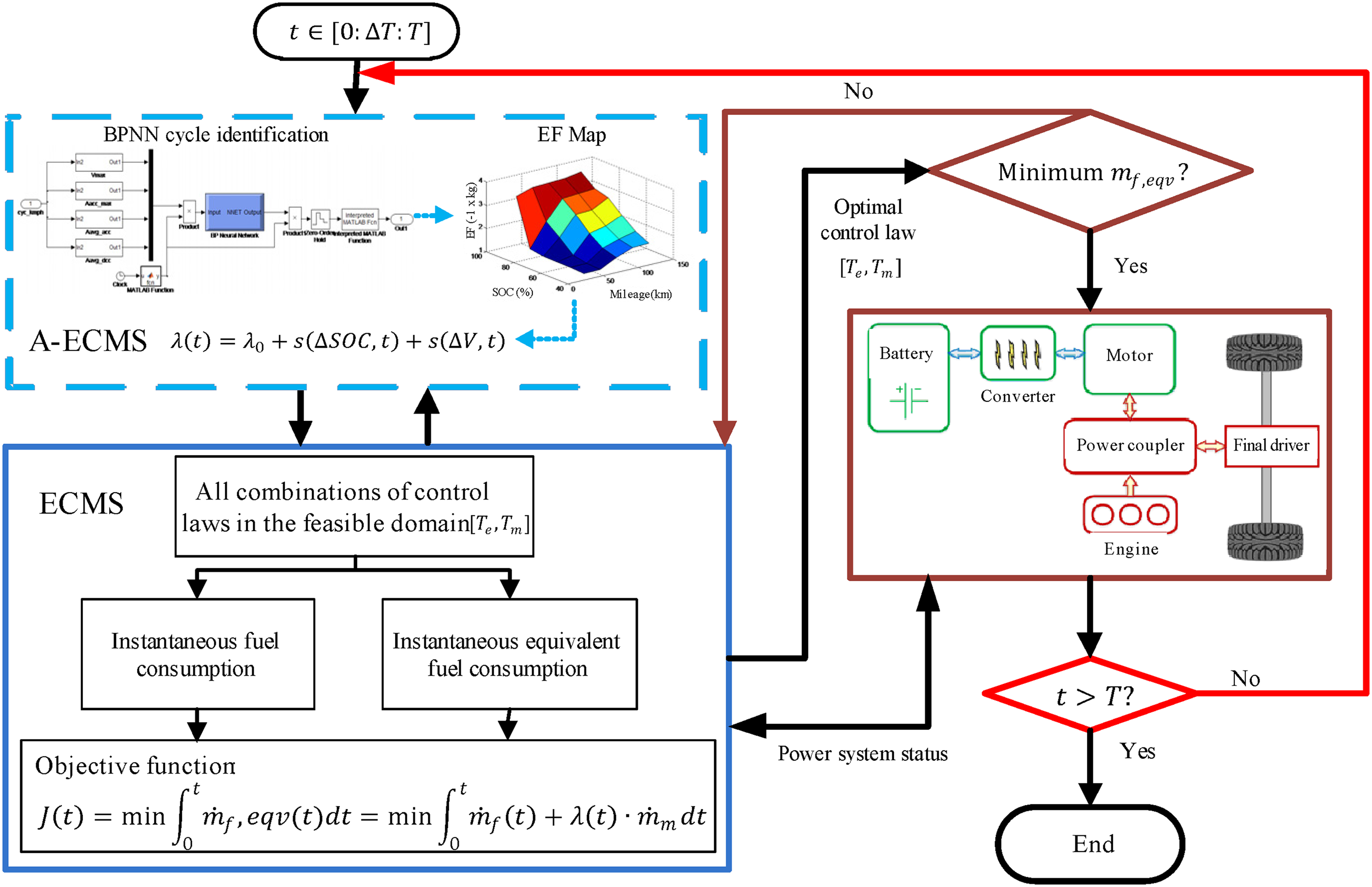
Working process of A-ECMS.

Since EF is obtained under a predefined cycle and requires a lot of calculations, these obviously cannot be applied online. In order to solve this problem, this paper uses GA to calculate EF MAP under certain specific cycles offline. In the actual driving event, the initial EF is obtained by interpolating in EF Map, then SOC penalty factor and velocity penalty factor are introduced for feedback adjustment, so as to achieve a fuel consumption level close to the optimal level.

Simulation results and discussions

The A-ECMS model is built by the MATLAB Function module, and Hamilton function was written in the M file, which was embedded into the model through the MATLAB Function module. Based on the control strategy model, this module communicates with the vehicle model by the AVL/Cruise, as displayed in Figure 22.

Figure 22.

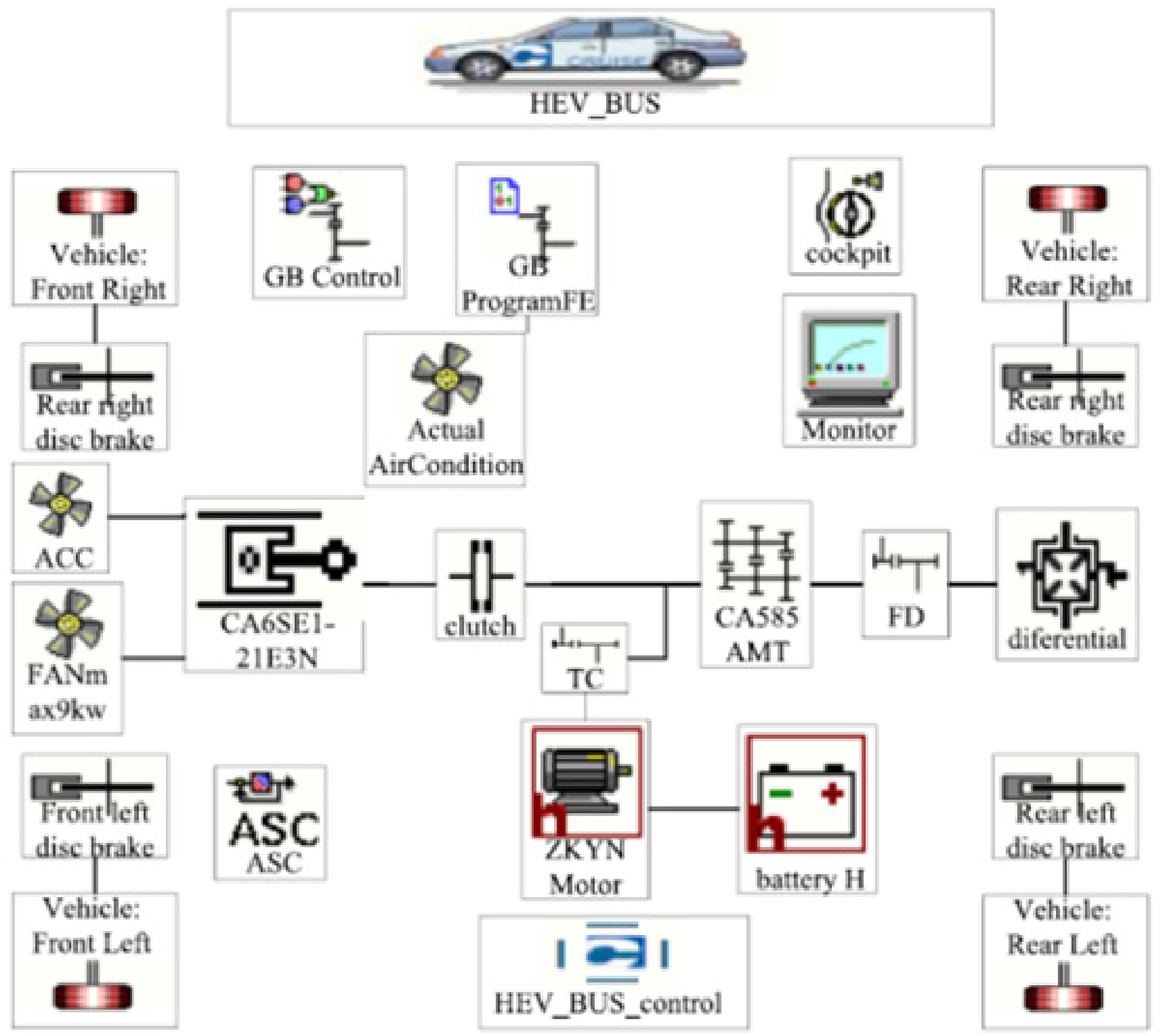
Vehicle model built in AVL/cruise software.

3*WLTC and 4*WLTC cycles are selected as simulation cycles, the initial SOC is set to 0.8, and the minimum available SOC is set to 0.4. Simulation results of ECMS and A-ECMS based on IRDC are analysed from the aspects of power performance, SOC, EF, engine working condition and fuel economy, respectively. EF is a fixed value in ECMS, and the Initial EF of ECMS is −1.82kg under 3*WLTC cycle.

Figure 23 shows the velocity of A-ECMS under 3*WLTC and 4*WLTC cycles. Velocity tracking effect is good. Although there has a deviation at the peak of velocity, the maximum difference is only 1.67 km/h, and the overall average error is less than 0.1 km/h.

Figure 23.

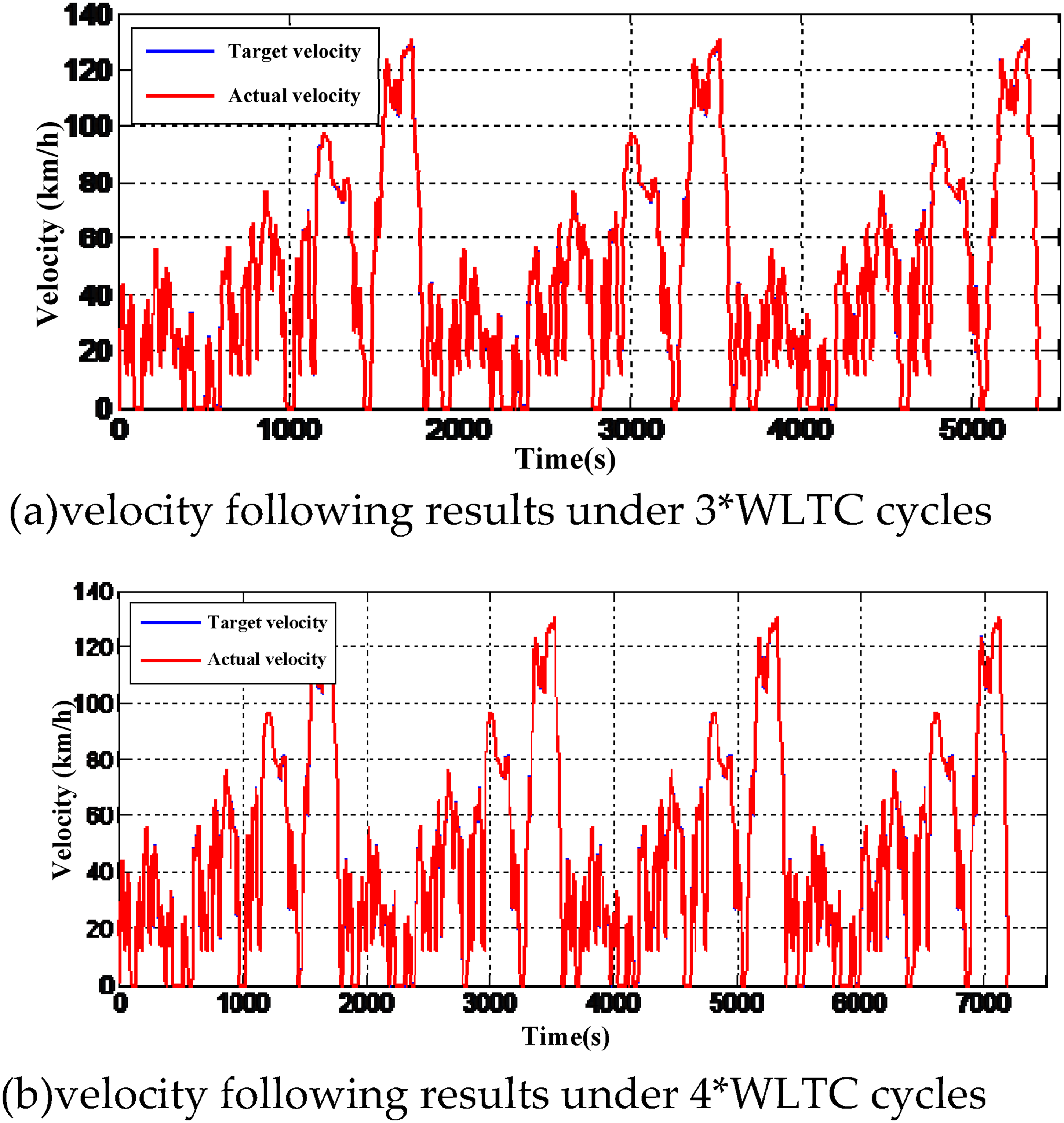
A-ECMS velocity following results. (a) EF variation curve with mileage under 3WLTC cycle. (b) EF variation curve with mileage under 4WLTC cycle.

Figure 24 depicts the variation of EF in A-ECMS with mileage under 3*WLTC and 4*WLTC cycles. It can be seen that SOC and speed penalty factor have corrected the EF, which is well implemented to ensure full and reasonable use of electricity.

Figure 24.

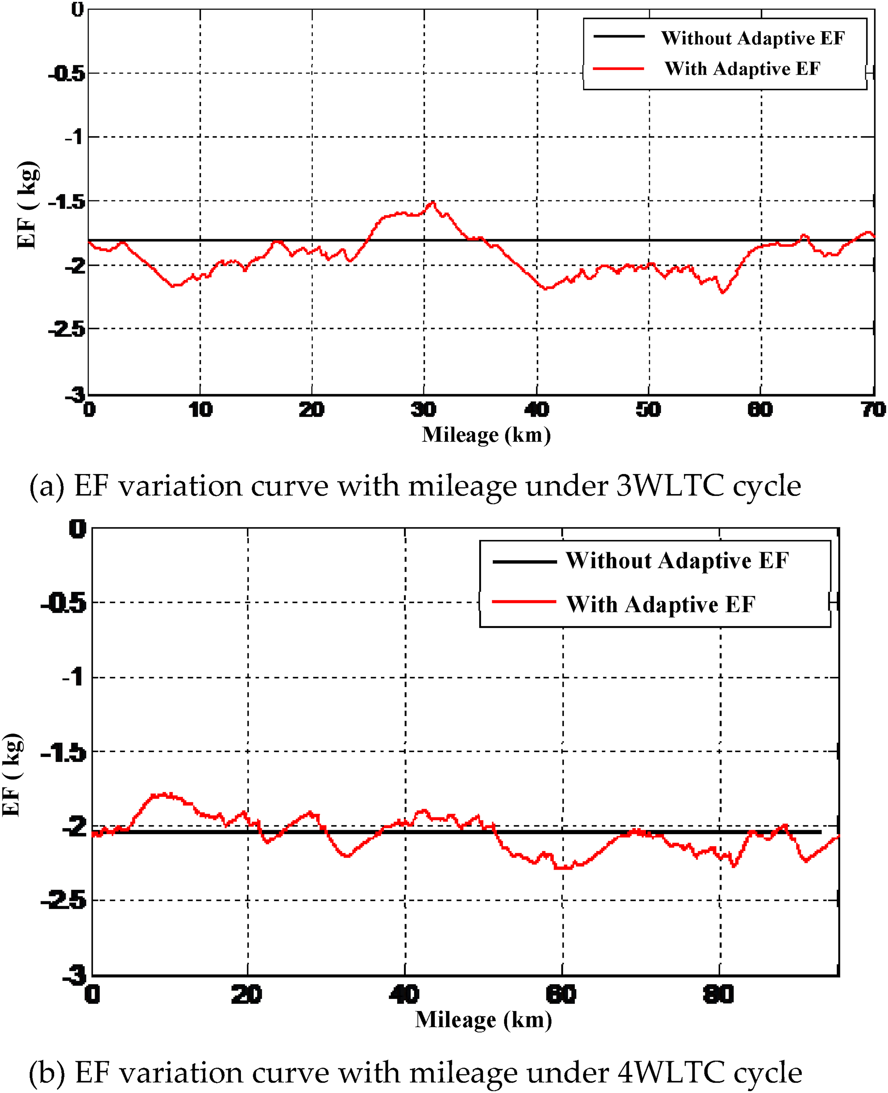
Ef variation curve of WLTC cycle. (a)ECMS engine workinging point and efficiency ratio. (b)A-ECMS engine workinging point and efficiency ratio.

Figure 25 and Figure 26 illustrate the distribution of engine working points and efficiency ratio of ECMS and A-ECMS under 3^*WLTC and 4^*WLTC cycles. Although ECMS improves fuel economy of PHEV and enables engine to operate in a more efficient working area, which is not as good as the A-ECMS in terms of fuel economy and engine working area at different mileage because its EF is fixed. Compared with engine working point distribution of ECMS, engine working point distribution of A-ECMS based on IRDC can be more concentrated in the efficient working area under both cycles, and the proportion of engine high efficiency is higher. This is mainly due to the ability of A-ECMS to automatically adjust EF according to mileage, thus optimally allocate engine and motor output torque, so that engine can operate in the efficient area throughout entire journey, which is the main reason for saving fuel consumption.

Figure 25.

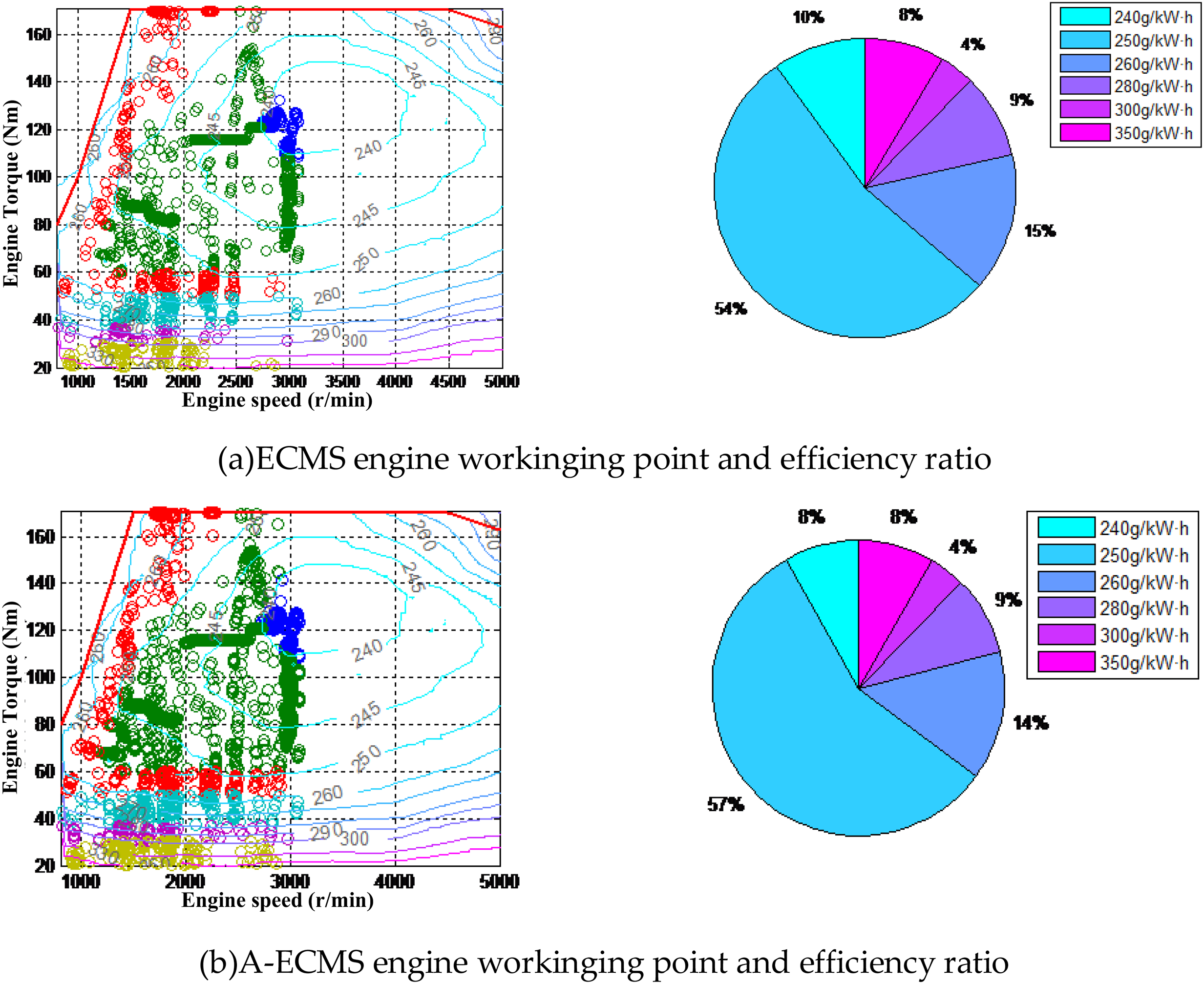
Distribution of engine working points and efficiency ratio under 3^*WLTC cycle. (a)ECMS engine workinging point and efficiency ratio. (b)A-ECMS engine workinging point and efficiency ratio.

Figure 26.

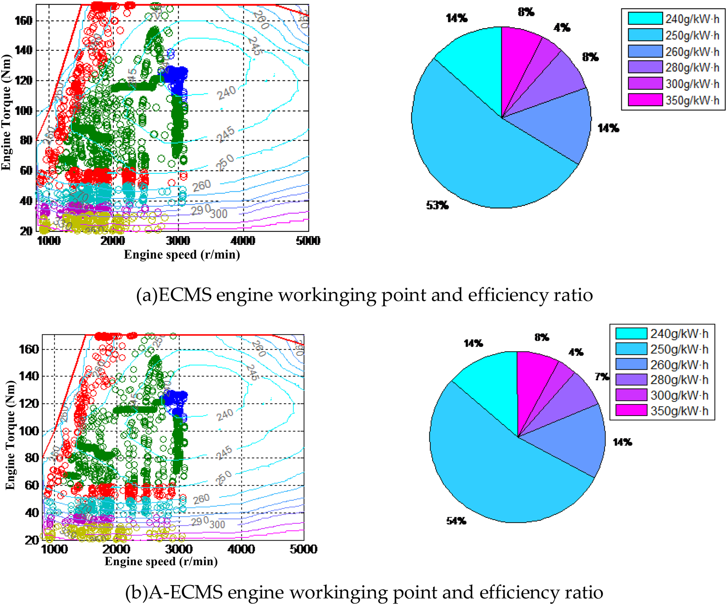
Distribution of engine working points and efficiency ratio under 4^*WLTC cycle.

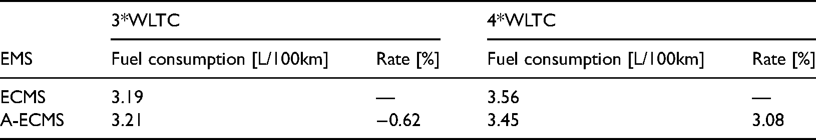
Table 8 lists fuel consumption of ECMS and A-ECMS under 3^*WLTC and 4^*WLTC cycles. under the 3^*WLTC cycle, fuel consumption of ECMS and A-ECMS is close to each other, and fuel saving rate of A-ECMS is slightly higher than that of ECMS by 0.62%. Under 4^*WLTC cycle, A-ECMS can be adaptatively adjusted according to mileage, and fuel saving rate is significantly higher than that of ECMS by 3.08%.

Table 8.

Fuel consumption of ECMS and A-ECMS under 3*WLTC and 4*WLTC cycles.

EMS	3*WLTC		4*WLTC
EMS	Fuel consumption [L/100km]	Rate [%]	Fuel consumption [L/100km]	Rate [%]
ECMS	3.19	—	3.56	—
A-ECMS	3.21	−0.62	3.45	3.08

Conclusions

In this paper, A-ECMS for PHEVs based on IRDC is proposed. Firstly, GA is employed to get EF Map in different conditions; Then, BPNN is utilized to identify driving cycles and selects the corresponding EF Map; Finally, SOC and velocity penalty factors are introduced for feedback adjustment, in order to maximize the use of electrical power. This paper can be summarized as follows.

Combined with PMP theory, designed ECMS based on PMP;

GA was employed to solve EF off-line under specific driving cycles and EF MAP was established, so that EF under actual driving events could be obtained by interpolation method;

A-ECMS based on reference SOC and IRDC is proposed, which considers the effects of SOC and mileage on EF, and introduces SOC penalty factor and velocity penalty factor to make EF adaptive adjustment;

A-ECMS was established based on Matlab/Simulink, and the principle was verified under WLTC cycle. simulation results show that compared with ECMS, the proposed strategy can reasonably plan SOC, adjust engine and motor power allocation proportion, make engine work in high efficient area. The fuel saving rate is up to 3%, which verifies that proposed A-ECMS is correct and effective.

Footnotes

Acknowledgements

This work was supported by Central Government of Hubei Province to Guide Local Science and Technology Development (2020ZYYD001), Guiding Project of Science and Technology Research Plan of Department of Education of Hubei Province (B2021210), Hubei Key Laboratory of Power System Design and Test for Electrical Vehicle (ZDSY202206).

Author contributions

In this paper, Changzheng Guo and Yinggang Xu analyse the optimization methods of different energy control strategies and determine the optimal control algorithm. Shipeng Li determines the configuration of PHEV and the research objectives of the power control system. Yun Wang analyses the energy control problem by the PMP theory and put forward the improvement measures for the energy control problem. Dapai Shi analyses the relationship between the equivalent fuel factor and reference SOC, and establishes the energy control model of the equivalent minimum fuel consumption by MATLAB/Simulink. Kangjie Liu simulate the PHEV simulation model by combining with Cruise and Simulink. All authors have read and agreed to the published version of the manuscript.

Data availability

The data that support the findings of this study are available from the corresponding author upon reasonable request

Declaration of conflicting interests

The author(s) declared no potential conflicts of interest with respect to the research, authorship, and/or publication of this article.

Funding

The author(s) disclosed receipt of the following financial support for the research, authorship, and/or publication of this article: This work was supported by the Hubei Key Laboratory of Power System Design and Test for Electrical Vehicle, Guiding Project of Science and Technology Research Plan of Department of Education of Hubei Province, Central Government of Hubei Province to Guide Local Science and Technology Development, (grant number ZDSY202206, B2021210, 2020ZYYD001).

ORCID iD

Kangjie Liu

References

Banvait

Anwar

Chen

(2009) A rule-based energy management strategy for plug-in hybrid electric vehicle (PHEV). In: American control conference, pp. 3938–3943: IEEE.

Bayindir

KÇ

Gözüküçük

Teke

(2011) A comprehensive overview of hybrid electric vehicle: Powertrain configurations, powertrain control techniques and electronic control units. Energy Conversion & Management 52(2): 1305–1313.

Chen

Liu

Yang

, et al. (2015) Online energy management of plug-in hybrid electric vehicles for prolongation of all-electric range based on dynamic programming. Mathematical Problems in Engineering 2015(1): 1–11.

Chen

Xiong

Wang

, et al. (2015) Optimal energy management strategy of a plug-in hybrid electric vehicle based on a particle swarm optimization algorithm. Energies 8(5): 3661–3678.

Guo

Wei

(2018) Study on HEV’s driving condition recognition method based on PSO algorithm. Journal of Intelligent & Fuzzy Systems 35(1): 87–98.

Kavya

Sanjaka

Ali

, et al. (2019) Artificial neural network based adaptive control for plug-in hybrid electric vehicles. International Journal of Electric and Hybrid Vehicles 11(2): 121–151.

Khayyam

Bab-Hadiashar

(2014) Adaptive intelligent energy management system of plug-in hybrid electric vehicle. Energy 69(5): 319–335.

Kim

Cha S

Peng

(2012) Optimal equivalent fuel consumption for hybrid electric vehicles. IEEE Transactions on Control Systems Technology 20(3): 817–825.

Kim

Rousseau

Lee

(2011) A jump condition of PMP-based control for PHEVs. Journal of Power Sources 196(23): 10380–10386.

10.

Lecce

Calabrese

(2009) NN-based measurements for driving pattern classification. In: 2009 IEEE Instrumentation and Measurement Technology Conference, pp. 259–264. IEEE.

11.

Liu

Chen

Zhan

, et al. (2019) Heuristic dynamic programming based online energy management strategy for plug-in hybrid electric vehicles. IEEE Transactions on Vehicular Technology 68(5): 4479–4493.

12.

Montazeri-Gh

Poursamad

Ghalichi

(2006) Application of genetic algorithm for optimization of control strategy in parallel hybrid electric vehicles. Journal of the Franklin Institute 343(4): 420–435.

13.

Montazeri-Gh

Fotouhi

Naderpour

(2011) Driving patterns clustering based on driving features analysis. Journal of Mechanical Engineering Science 225: 1301–1317.

14.

Moura

Fathy

Callaway

, et al. (2011) A stochastic optimal control approach for power management in plug-in hybrid electric vehicles. IEEE Transaction on Control Systems Technology 19(3): 545–555.

15.

Nuesch

Wang

Isenegger

, et al. (2014) Optimal energy management for a diesel hybrid electric vehicle considering transient PM and quasi-static NOx emissions. Control Engineering Practice 29(SI): 266–276.

16.

Onori

Serrao

Rizzoni

(2016) Pontryagin’s minimum principle. In Hybrid Electric Vehicles. London: Springer, pp. 51–63.

17.

Ouddah

Adouane

Abdrakhmanov

(2018) From offline to adaptive online energy management strategy of hybrid vehicle using pontryagin's minimum principle. International Journal of Automotive Technology 19(3): 571–584.

18.

Panday

Bansal

(2016) Energy management strategy for hybrid electric vehicles using genetic algorithm. Journal of Renewable & Sustainable Energy 8(1): 741–646.

19.

Poursamad

Montazeri

(2008) Design of genetic-fuzzy control strategy for parallel hybrid electric vehicles. Control Engineering Practice 16(7): 861–873.

20.

Yin

Zhang

(2007) Optimal control of fuel economy in parallel hybrid electric vehicles. Proceedings of the Institution of Mechanical Engineers. Part D: Journal of Autombile Engineering 221(10): 1097–1106.

21.

Sabri

MFM

Danapalasingam

Rahmat

(2016) A review on hybrid electric vehicles architecture and energy management strategies. Renewable & Sustainable Energy Reviews 53: 1433–1442.

22.

Serrao

Onori

Rizzoni

(2009) ECMS as a realization of Pontryagin's minimum principle for HEV control. In: American control conference, pp. 3964–3969: IEEE.

23.

Sorrentino

Rizzo

Arsie

(2011) Analysis of a rule-based control strategy for on-board energy management of series hybrid vehicles. Control Engineering Practice 19(12): 1433–1441.

24.

Sun

(2017) Investigating adaptive-ECMS with velocity forecast ability for hybrid electric vehicles. Apply Energy 185: 1644–1653.

25.

Sun

Lin

(2017) Energy management strategy based on type recognition and multivariate nonlinear regression optimization. China Mechanical Engineering 28(22): 2695.

26.

Trovão

Pereirinha

Jorge

, et al. (2013) A multi-level energy management system for multi-source electric vehicles – an integrated rule-based meta-heuristic approach. Applied Energy 105: 304–318.

27.

Tulpule

Marano

Rizzoni

(2010) Energy management for plug-in hybrid electric vehicles using equivalent consumption minimization strategy. International Journal of Electric and Hybrid Vehicles 2(4): 329–350.

28.

Wang

Zeng

, et al. (2015) Driving cycle recognition neural network algorithm based on the sliding time window for hybrid electric vehicles. International Journal of Automotive Technology 16(4): 685–695.

29.

Wang

Yang

(2019) Simulation of Energy Control Strategy for Hybrid Electric Vehicle Based on Modified Dynamic Programming. In: 3rd Conference on Vehicle Control and Intelligence (CVCI), pp. 1–4: IEEE.

30.

Wang

Zeng

Song

(2020) Hierarchical optimal intelligent energy management strategy for a power-split hybrid electric bus based on driving information. Energy 199: 117499.

31.

Zhang

Cui

(2012) Fuzzy energy management strategy for a hybrid electric vehicle based on driving cycle recognition. International Journal of Automotive Technology 13(7): 1159–1167.

32.

Xie

Tian

, et al. (2018) A hybrid method combining markov prediction and fuzzy classification for driving condition recognition. IEEE Transactions on Vehicular Technology 67(11): 10411–10424.

33.

Xie

, et al. (2018) An artificial neural network-enhanced energy management strategy for plug-in hybrid electric vehicles. Energy 163: 837–848.

34.

Zeman

(2012) Modeling and optimization of plug-In hybrid electric vehicle fuel economy. In: SAE 2012 World Congress and Exhibition, (No. 2012-01-1018). SAE Technical Paper.

35.

Zhan

Qin

Zeng

(2016) Energy management strategy of HEV based on driving cycle recognition using genetic optimized K-means clustering algorithm. China Journal of Highway and Transport 29(4): 130.

36.

Zhang

Dong

, et al. (2014) Embedded feature-selection support vector machine for driving pattern recognition. Journal of the Franklin Institute 352(2): 669–685.

37.

Zhang

Yan

(2015) A comprehensive analysis of energy management strategies for hybrid electric vehicles based on bibliometrics. Renewable & Sustainable Energy Reviews 48: 88–104.

38.

Zhang

, et al. (2020) Adaptive equivalent consumption minimization strategy for hybrid heavy-duty truck based on driving condition recognition and parameter optimization. Energies 13(20): 1–20.

Adaptive energy management strategy for plug-in hybrid electric vehicles based on intelligent recognition of driving cycle

Abstract

Keywords

Introduction

Model of IRDC

Construction of comprehensive driving cycles

Driving cycle identification model

BPNN driving cycle identification model

Simulation and comparative analysis

Design of A-EMS

Establishment and solution of optimal objective function

Establishment of optimal objective function

Solution optimal objective function

Design of ECMS

Calculation of EF and establishment of EF map diagram

Calculation of EF

Establishment of EF map diagram

Design and establishment of A-ECMS

Design of A-ECMS

Establishment of A-ECMS

Simulation results and discussions

Conclusions

Footnotes

Acknowledgements

Author contributions

Data availability

Declaration of conflicting interests

Funding

ORCID iD

References