Sage Journals: Discover world-class research

Abstract

In this study, we analyse the impact of oil price uncertainty (as measured by an observable measure of oil price volatility, i.e. realised volatility) on United States state-level real consumption by accounting for oil dependency. We account for both the long- and short-run dynamics of the state-level consumption function using the panel Pooled Mean Group estimator. The analysis makes use of a novel dataset including housing and stock market wealth at the state level covering the quarterly period 1975:Q1 to 2012:Q2, supplemented with an annual dataset up to 2018. We simultaneously estimate the long-run relationship and short-run impact of oil price volatility at the state-level conditional upon their oil dependency. We find that the negative impact of volatility is most severe for the states of Wyoming, Alaska and New Mexico, while the negative impact is least for Illinois, New York and Nebraska. States with lower per capita income and consumption expenditure, notably in the Southeast and Southwest region of the country are exposed to be more vulnerable to the negative impact of adverse developments and uncertainty in the oil market, as they may have less access to a stock of wealth and other means as recourse. Heterogenous responses, therefore, necessitate additional state-level response besides the national response to oil uncertainty.

Keywords

Oil price volatility oil dependency U.S. state-level consumption

Introduction

In a recent paper De Michelis et al. (2020), inter alia, analysed for the first time the impact of oil price on a panel data set of state-level consumption (proxied by registration of new cars) of the United States (U.S.), by accounting for oil dependency (calculated as oil consumed minus oil produced as percentage of oil consumed) of these states. They show that the benefits from oil-price decreases are smaller than the losses from oil-price increases across the U.S. states. The study also finds that shocks pushing up oil prices are followed by a national decrease in car registrations with this decline being larger than the increase in registrations following a comparable oil price drop. In sum, the state-level evidence highlighted the fact that varying oil dependency may imply differences in consumption responses across regions following oil price shocks, when one might expect that common monetary and fiscal policies would drive similar regional responses. Against this backdrop, the objective of our study is to analyse the impact of oil price uncertainty (as measured by an observable measure of oil price volatility, i.e., realised volatility) on state-level consumption by accounting for oil dependency. In this regard, we model both the long- and short-run dynamics of the state-level consumption function using a panel data approach over the quarterly period of 1975:Q1 to 2012:Q2,¹ and simultaneously estimate the short-run impact of oil price volatility at the state-level conditional upon their oil dependency.

Intuitively, the effect of oil price uncertainty (volatility) on economic activity is generally explained by the real option theory (see for example, Bernanke (1983), Pindyck (1991), and Dixit and Pindyck (1994)), which suggests that decision-making is affected by uncertainty because it raises the option value of waiting. In other words, given that the cost associated with wrong investment decisions is very high, uncertainty makes firms and, in the case of durable goods, also consumers more cautious. As a result, economic agents postpone investment, hiring and consumption decisions for precautionary savings reasons to periods of lower uncertainty, which results in cyclical fluctuations in macroeconomic aggregates (Punzi, 2019). In other words, oil price uncertainty is expected to negatively impact consumption (as well as investment and overall output).²

Note that, while effects of oil price uncertainty on aggregate and disaggregate consumption of the overall U.S. has been analysed before (see for example, Guo and Kliesen (2005), Elder and Serletis (2010), Kilian and Vigfusson (2011)), to the best of our knowledge this is the first study to analyse the state-level impact of oil price volatility accounting for oil dependency. The remainder of the paper is organized as follows: the next section discusses the data, followed by the methodology and empirical results, with the final section concluding the paper.

Data

In this paper, we employ the state-level data for household consumption, financial wealth, owner-occupied housing wealth and personal income from Case et al. (2005, 2013). Due to data availability, there are two main limitations of the dataset: (i) households' consumption spending is proxied by total retail sales; and (ii) households' financial wealth includes holdings of mutual funds only, which are mostly interpolated. Despite these features of the data that Case et al. (2013) acknowledges, it is important to note that this is virtually the only dataset that contains unique information about aggregate wealth (and its composition) for each of the 50 U.S. states (plus D.C.) and over a relatively long time-span covering the quarterly period of 1975:Q1–2012:Q2. Note that, we could not use the data set of De Michelis et al. (2020) to proxy consumption as it is not publicly available, besides the fact that there is no other data source besides the one of Case et al. (2005, 2013), which includes state-level information of stock wealth and housing wealth, required to appropriately model our consumption function.³ To address potential concerns regarding the robustness of findings when extending the sample period beyond the end of the novel dataset of Case et al. (2005, 2013), we perform an annual state-level analysis for the U.S. over the sample period 1975 to 2018, which supports the quarterly results at the state level.

In addition, we construct a realised volatility series using the daily data of West Texas Intermediate (WTI) oil price obtained from the Global Financial Database. In this regard, we follow Andersen and Bollerslev (1998), and compute realised volatility from the sum of daily squared log-returns of the oil price over a specific quarter. This approach provides an observable measure of oil market volatility unlike conditional volatility obtained from generalised autoregressive conditional heteroscedasticity (GARCH)-type models, which in turn tends to make volatility model specific. Following De Michelis et al. (2020), we also construct a state-specific oil dependency series using U.S. Energy Information Administration (EIA) data on oil production and oil consumption. Variables names with descriptions and sources are depicted in Table 1.

Table 1.

Data series used.

Variable name	Description	Source
c	Per capita consumption expenditure, proxied by retail sales per capita (constant US$, base 2000:2)	Case et al. (2013)
inc	Per capita personal income (constant US$, base 2000:2, in thousands)	Case et al. (2013)
hw	Housing wealth per capita (constant US$, base 2000:2)	Case et al. (2013)
sw	Stock holdings per capita (constant US$, base 2000:2)	Case et al. (2013)
wtirv	West Texas Intermediate oil price realised volatility calculated as the sum of daily squared log-returns over a quarter	Global Financial Database
odep	Oil dependency calculated as oil consumed minus oil produced as ratio of oil consumed^a	U.S. Energy Information Administration (EIA)
ocons	Oil consumption (all petroleum goods) (thousands of barrels daily)	U.S. Energy Information Administration (EIA)
oprod	Production of crude oil (thousands of barrels daily)	U.S. Energy Information Administration (EIA)
wtirv_odep	Realised volatility conditional on oil dependency (Interaction term of realised volatility of oil price and oil dependency after both series has been normalised using min-max option in Stata, i.e. normalised values ranges between 0 and 1.)

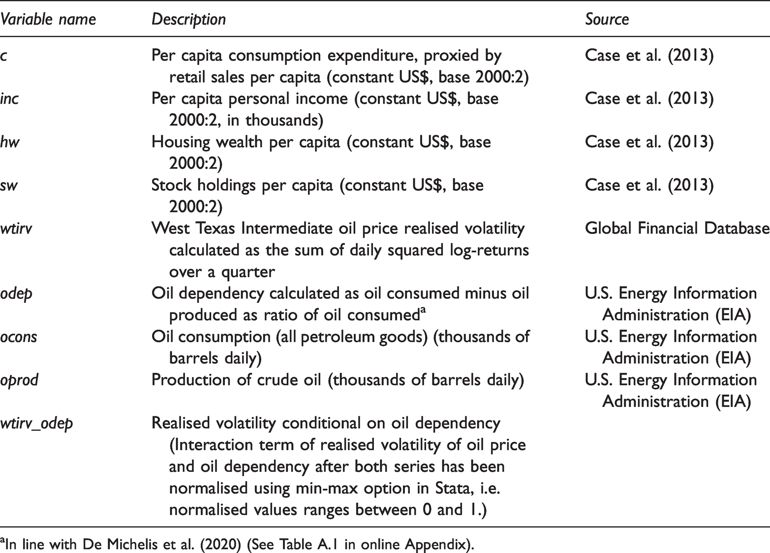
^aIn line with De Michelis et al. (2020) (See Table A.1 in online Appendix).

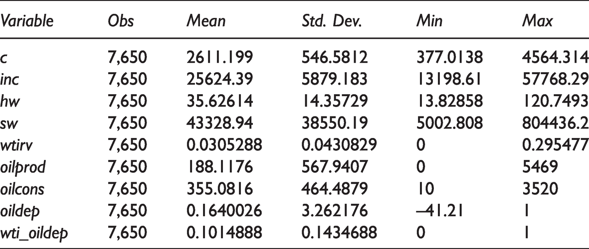
Descriptive statistics are reported in Table 2. The average consumption per capita across all states over the sample period (expressed in constant 2000 dollars) amounts to $2,611. A minimum value of $337 was recorded in the state of Tennessee in 1982, with a high of $4,564 recorded in New Hampshire in 2006. The average income per capita is $25,624 varying between a low of $13,199 in Mississippi and a maximum of $57,768 in the District of Columbia. The average housing wealth per capita across all states is $35.62, while the average stock market wealth per capita is $43,328.

Methodology and empirical results

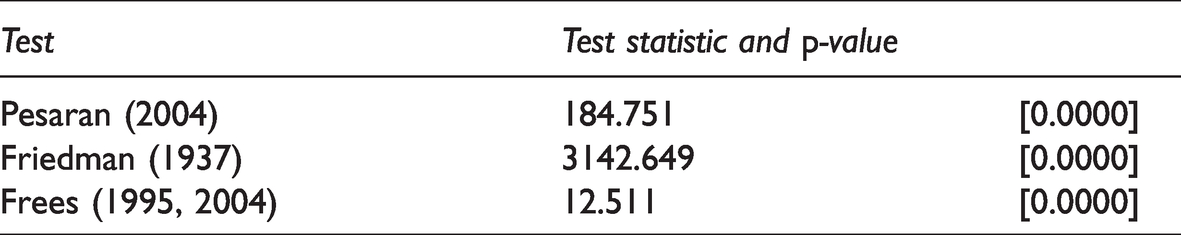
We inspect the univariate characteristics of the data using Pesaran’s (2007) second generation CIPS unit root test, based on the fact that there is evidence of the existence of cross-sectional dependence. All three tests in Table 3 provide support for the existence of cross-sectional dependence by rejecting the null of cross-sectional independence at the one per cent level (Frees, 1995, 2004; Friedman, 1937; Pesaran, 2004). This result is expected given that all states form part of a single country and flows of goods and services, bootlegging behaviour of consumers, and spillover effects of uncertainty can easily occur.

From Table 4, we conclude that the state-level consumption and income panels are non-stationary I(1), as we reject the null of a unit root after differencing the variables once. This serves as justification to include these variables in the long-run steady-state component of an error correction model. The variables of interest, oil price uncertainty, wtirv, and oil price uncertainty conditional on oil dependency, wti_oildep, are both stationary and will be included in the short-run component of the error correction model to test the impact that increased volatility will exert on state-level consumption. All unit root test specifications include cross-sectional and first-difference means for the variable under inspection and a deterministic constant in the test regression.

Table 2.

Descriptive statistics.

Variable	Obs	Mean	Std. Dev.	Min	Max
c	7,650	2611.199	546.5812	377.0138	4564.314
inc	7,650	25624.39	5879.183	13198.61	57768.29
hw	7,650	35.62614	14.35729	13.82858	120.7493
sw	7,650	43328.94	38550.19	5002.808	804436.2
wtirv	7,650	0.0305288	0.0430829	0	0.295477
oilprod	7,650	188.1176	567.9407	0	5469
oilcons	7,650	355.0816	464.4879	10	3520
oildep	7,650	0.1640026	3.262176	–41.21	1
wti_oildep	7,650	0.1014888	0.1434688	0	1

Table 3.

Cross-sectional dependence tests.

Test	Test statistic and p-value
Pesaran (2004)	184.751	[0.0000]
Friedman (1937)	3142.649	[0.0000]
Frees (1995, 2004)	12.511	[0.0000]

Table 4.

Panel unit root tests results in the presence of cross-sectional dependence.

Variable	CIPS test statistic	Variable	CIPS test statistic
lc	–1.527	Δlc	–5.441***
linc	–1.667	Δlinc	–6.136***
lhw	–1.945	Δlhw	–6.171***
lsw	–1.868	Δlsw	–3.589***
wtirv	–4.531***
wtirv_odep	–4.530***

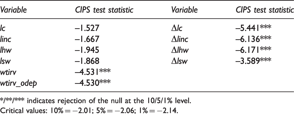
*/**/*** indicates rejection of the null at the 10/5/1% level.

Critical values: 10% = −2.01; 5% = −2.06; 1% = −2.14.

Given the non-stationary properties of income and consumption data, we specify an error correction model for consumption, in line with Case et al. (2013), but add (state-invariant) realised oil price volatility to the equation:

Δ {lnc}_{i t} = \propto_{i} Δ {lnc}_{i, t - 1} + {β 1}_{i} Δ {lninc}_{i t} + {β 2}_{i} {Δ lnsw}_{i t} + {β 3}_{i} {Δ lnhw}_{i t} {+ β 4}_{i} {wtirv}_{i t} + γ ({lnc}_{i, t - 1} - {θ lninc}_{i, t - 1}) + μ_{i} + ε_{i t}

(1)

Additionally, we model the impact of oil price volatility on consumption conditional on the level of oil dependency of individual states, by interacting the realised oil price volatility measure with oil dependency:

{lnc}_{i t} = \propto_{i} Δ {lnc}_{i, t - 1} + {β 1}_{i} Δ {lninc}_{i t} + {β 2}_{i} {Δ lnsw}_{i t} + {β 3}_{i} {Δ lnhw}_{i t} {+ β 4}_{i} {(wtirv}_{i t} \times {oildep}_{i t}) + γ ({lnc}_{i, t - 1} - {θ lninc}_{i, t - 1}) + μ_{i} + ε_{i t}

(2)

Consumption, as well as housing and stock market wealth variables, are expressed in natural logarithmic form, while the realised oil price volatility variable, wtirv, is standardised to be constrained to the [0,1] range. The same holds for the interaction term, wtirv×oildep. $μ_{i}$ represents the unobservable country-specific effect, and $ε_{i t}$ is the stochastic disturbance term. All coefficients with subscripts i represent short-run state-specific results of the relationship between variables.

We start by addressing heterogeneity concerns, with real income and real consumption levels varying substantially across U.S. states (refer to minimum and maximum values in Table 2 with descriptive statistics). Likewise, notable differences exist in oil dependency levels across states. Moreover, numerous oil price shocks have been recorded over the sample period, justifying testing for the validity of time effects in addition to that of state effects. Results are reported in Table 5.

Table 5.

Tests for validity of state-specific effects and time effects.

Null hypothesis	Test statistic and p-value
H₀: µ₁ = µ₂ = ⋯ = µ_N-1 = 0	F(50, 7596) = 2831.520 [0.000]
H₀: λ₁ = λ₂ = ⋯ = λ_T-1 = 0	F(149, 7497) = 0.890 [0.826]

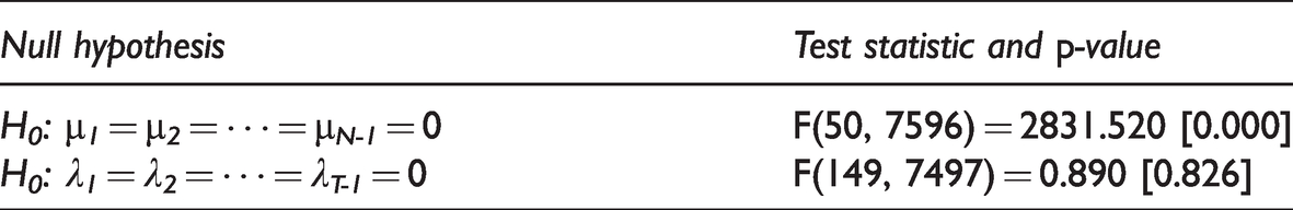
We reject the null that state-level effects are jointly significantly different from zero. However, when considering time effects on its own, there is no strong evidence for dynamic adjustment over time. When testing for time effect while controlling for state effects, there is evidence of the validity of time effects. For this reason, we make use of a two-way error component model to obtain the long-run residual to construct an error correction model (ECM) as a robustness check for the estimation results reported in Table 7. The results are qualitatively similar.

Table 7.

Pooled Mean Group estimation across all U.S. states, 1975Q1 to 2012Q2.^a

	(1)	(2)
	D.lc	D.lc
ec
linc	0.825***	0.826***
	(38.20)	(38.26)
S.R.
ec	–0.0516***	–0.0516***
	(–18.75)	(–18.68)
D.lag_lc	0.0141	0.0139
	(1.01)	(0.99)
D.linc	0.406***	0.406***
	(21.02)	(21.01)
D.lsw	0.0279***	0.0278***
	(13.46)	(13.38)
D.lhw	0.105***	0.105***
	(8.85)	(8.86)
wtirv	–0.0234***(–23.41)
wtirv_odep		–0.0242***(–21.92)
_cons	–0.0229***	–0.0236***
	(–17.27)	(–17.49)
Obs	7548	7548
Number of groups	51	51

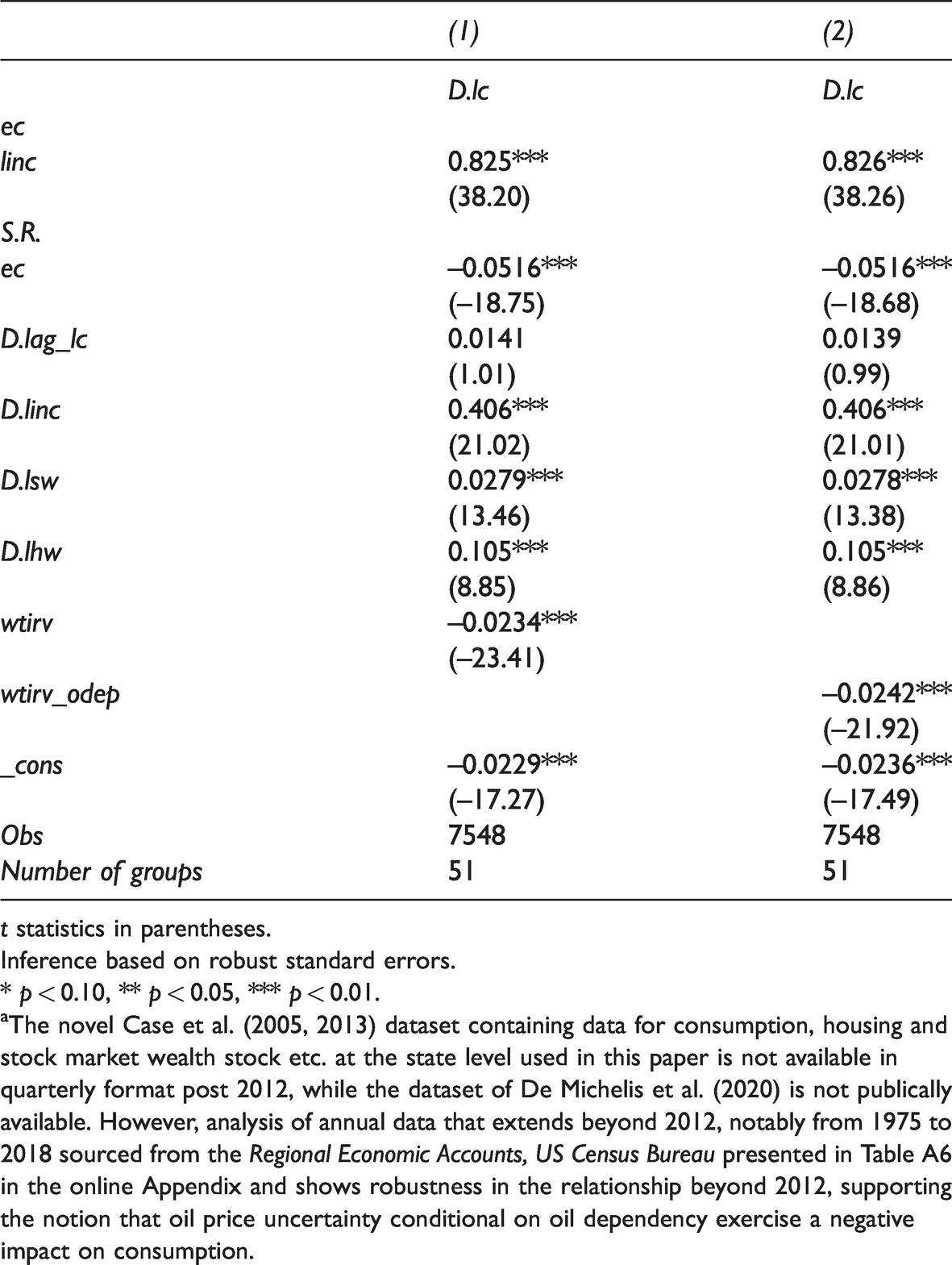
t statistics in parentheses.

Inference based on robust standard errors.

* p < 0.10, ** p < 0.05, *** p < 0.01.

^aThe novel Case et al. (2005, 2013) dataset containing data for consumption, housing and stock market wealth stock etc. at the state level used in this paper is not available in quarterly format post 2012, while the dataset of De Michelis et al. (2020) is not publically available. However, analysis of annual data that extends beyond 2012, notably from 1975 to 2018 sourced from the Regional Economic Accounts, US Census Bureau presented in Table A6 in the online Appendix and shows robustness in the relationship beyond 2012, supporting the notion that oil price uncertainty conditional on oil dependency exercise a negative impact on consumption.

In recent years, the dynamic panel data literature has begun to focus on panels in which both the cross-sectional (N) and time (T) dimensions are large. Blackburn and Frank (2007) point out the asymptotics for large N, large T dynamic panels are different to the traditional panels with large N and small T. Small T panel estimation typically relies on fixed effects or random effects estimators, or a combination of fixed effects and instrumental variable estimators. These methods entail pooling individual groups and only allowing for the intercepts to vary across groups. An important finding of the large N, large T literature, however, is that assuming homogeneity of the slope coefficients often is inappropriate (see for instance Im et al., 2003; Pesaran and Smith, 1995; Pesaran et al., 1997, 1999; Phillips and Moon, 2000). Also of concern with the increase of time observations is the issue of nonstationarity. Persaran et al., (1997, 1999) offer techniques to estimate non-stationary dynamic panels in which the parameters are homogeneous across groups. The mean group (MG) estimator relies on estimating N time series regressions and averaging the coefficients, while the pooled mean group (PMG) estimator relies on a combination of pooling and averaging of coefficients. Specifically, the technique allows for the pooling of the long-run coefficients − the income elasticity of consumption, i.e. the marginal propensity to consume, in this instance − while all other parameters are cross-section specific, including the error correction mechanisms (also referred to as the error-correcting speed of adjustment terms), other short-run coefficients and intercept terms. Since the error correction model is nonlinear in the parameters, Pesaran et al. (1999) propose a maximum likelihood method to estimate the parameters.

In this study we make use of Pesaran et al.’s (1997, 1999) Pooled Mean Group (PMG) estimator to account for the long-run steady-state relationship that exists between per capita consumption and income as dictated by economic theory, but also for the short-run dynamic adjustment impacts of housing and stock market wealth as well as oil price uncertainty and oil dependency. Lagged consumption is also included to account for habit persistence in consumption expenditure behaviour. In typical consumption analysis the parameters of primary interest would be the long-run coefficient, θ, and the error-correction speed of adjustment parameter, γ (see for instance Pesaran et al., 1997, 1999). Case et al. (2005, 2013) compare the housing wealth effect with the stock market wealth effect and report that the housing wealth effect is more pronounced than that of stock market wealth. In this study, we focus on the impact of oil price volatility and oil dependency on consumer expenditure, as proxied by retail sales. The cointegration results are contained in Table 6, and the PMG estimation results are reported in Table 7 for models specified in equations (1) and (2), displaying the common long-run income elasticity and the averaged short-run parameter estimates.⁴

Table 6.

Panel cointegration test results.

	Test statistic	Test statistic and p-value
Kao (1999)H₀: No cointegrationH_A: All panels are cointegrated	Modified Dickey-Fuller t Dickey-Fuller tAugmented Dickey-Fuller t Unadjusted modified Dickey-Fuller t Unadjusted Dickey-Fuller t	−7.8729 [0.0000] −4.3535 [0.0000] −9.4527 [0.0000] −5.0342 [0.0000] −3.3446 [0.0004]
Pedroni (2004) H₀: No cointegrationH_A: All panels are cointegrated	Modified Phillips-Perron t Phillips-Perron t Augmented Dickey-Fuller t	−1.1906 [0.1169] −1.8853 [0.0297] −2.3531 [0.0093]

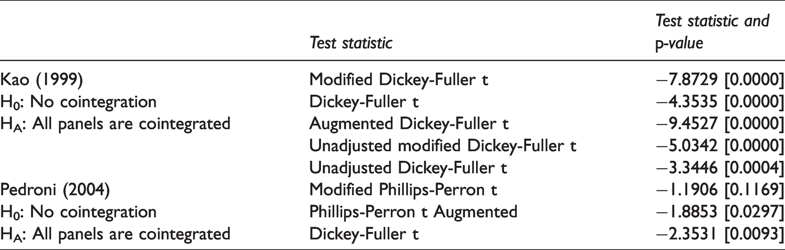
Based on the Kao (1999) and Pedroni (2004) cointegration tests, we reject the null of no cointegration in favour of the existence of a long-run cointegrated relationship between per capita real consumption expenditure and real personal income.

For the period under consideration, the income elasticity, or marginal propensity to consume, is equal to 0.8 in both models. All other parameters are also almost identical for the two model specifications, and all coefficients are statistically significant at the 1 per cent level. The error-correction speed of adjustment parameter is negative, implying that the variables in the long-run equation exhibit a return to long-run equilibrium, albeit at a slow rate given that the coefficient is closer to zero than to one in absolute terms. The average impact of realised oil price volatility is negative on consumption growth, so is its average impact conditional on the oil dependency of individual states.

It is however of interest to analyse the impact on the macroeconomy, or consumer behaviour specifically, of developments in the oil market, based on the fact that a number of states in the U.S. are oil producers, some of them in a significantly large volume (like Texas, Alaska, North Dakota, New Mexico, Oklahoma and others) while other states have no oil-producing capacity. The oil dependency of states also varies substantially (refer to Table A1 in the online Appendix for average oil production, oil consumption and oil dependency figures).

When considering the full result, with state-specific short-run results, all state-specific error-correction speed of adjustment parameters are negative and statistically significant at conventional levels. Parameters for wtirv and wtirv_oildep are negative and statically significant, with the exception of Illinois Michigan, Nebraska, New York, Utah and Washington, which also turns out to be the six states recording the lowest negative impact of oil price volatility and oil dependency on consumption expenditure.⁵

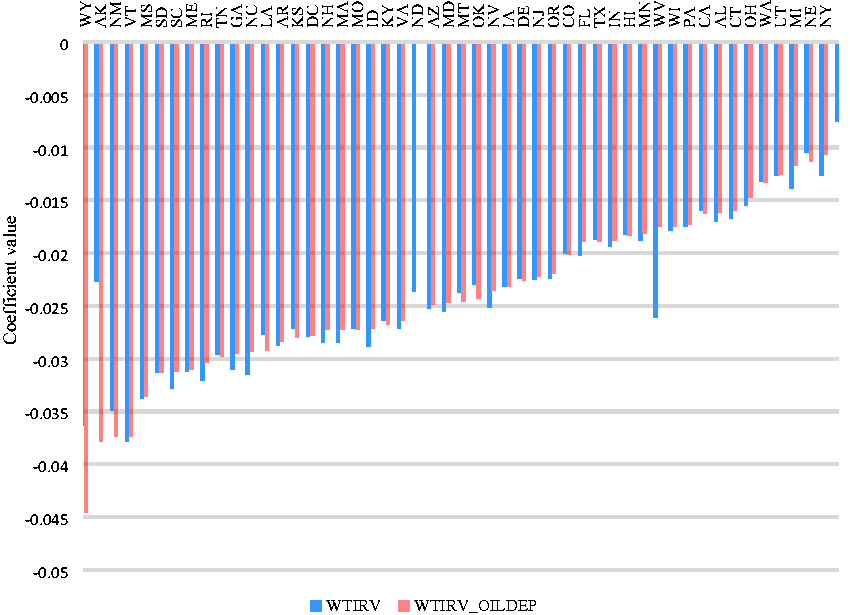
The coefficients representing the relative magnitude of the negative impact of oil price volatility on consumption, as well as that of oil price volatility conditional on oil dependency – our principal interest in this study – are depicted in Figure 1. The impact of oil price volatility, wtirv, is represented by coefficient ${β 4}_{i}$ in equation (1) and the impact of oil price volatility conditional on oil dependency, wtirv_oildep, as represented by coefficient ${β 4}_{i}$ in equation (2)). The rankings of impact are contained in Table A2 in the online Appendix.

Figure 1.

The impact of realised oil price volatility and realized volatility conditional on oil dependency on consumption, by state (ranked by wtirv × oildep).

The five states being impacted most negatively by oil price volatility are Vermont, Wyoming, New Mexico, Mississippi and South Carolina. Of these, Wyoming, New Mexico and Mississippi are also important oil producers. When also taking the oil dependency of the states into account, Wyoming, New Mexico and Mississippi again appear amongst the top five states being most severely negatively impacted. However, Alaska, the second largest oil-producing country, also enters the list, moving up from position 30 in the ranking of the impact of only oil price volatility.

Texas and California, despite being large oil producers, are not amongst the states most harshly impacted, but they rank somewhat lower in terms of oil dependency and rank higher in income and consumption.

The outcome of Vermont in the first analysis is somewhat surprising given that the state does not produce oil, nor does it rank high in terms of oil consumption and oil dependency. When taking West Virginia’s oil dependency into account, the impact seems less severe (West Virginia moves from position 22 to position 40).

Amongst the states ranking highest in terms of the negative impact of oil market development are also a number of states ranking low in terms of per capita income and per capita consumption. These include New Mexico, Tennessee, South Dakota, Louisiana, Mississippi, Arkansas. The latter three states also rank low in terms of housing wealth per capita. At the same token, several states rank high in terms of negative oil uncertainty impact and rank low on stock market wealth. These states include New Mexico, Wyoming, Louisiana, Arkansas, Tennessee, Georgia, South Dakota and North Dakota.

The results, therefore, suggest that oil-producing states might be more severely impacted by oil price uncertainty. A low number for the oil dependency measure is, therefore, an indication that the countries production exceeds the consumption by some margin, and may hint towards possible exposure in terms of the dependence of the state in selling its oil to neighbouring states or on the international market. Furthermore, the states with lower per capita income and consumption expenditure also appear to be more vulnerable to the negative impact of negative developments and uncertainty in the oil market, as they may have less access to a stock of wealth and other means of recourse.

From the spatial analysis portrayed in the Figures A1 to A4 in the online Appendix, the overlap is evident between low income−low consumption states and states with a sizable negative impact of oil price uncertainty on real consumption, reflected by states being lighter shaded. These states notably include Arkansas, Mississippi, Louisiana, Tennessee, South Carolina, New Mexico, and Idaho. North Carolina and Georgia are also among the states more severely impacted by oil uncertainty, although they rank slightly higher on income and consumption. With the exception of Idaho, all these states are in the Southeast and Southwest regions, traditionally regions with the highest poverty levels in the country.

Wyoming and Alaska, the two states that rank first and second in terms of the negative impact on consumption are exceptions in that these are wealthier states. The latter two states are however, both large oil producers and the two states where production exceeds consumption by the largest margin. What is clear is the heterogeneous nature of the negative impact of oil price uncertainty on macroeconomic outcomes in general, and consumption expenditure specifically.

Conclusion

This paper studies the effects of oil price uncertainty and oil dependency on consumption as proxied by retail sales across U.S. states. De Michelis et al. (2020) show that benefits from oil price decreases are smaller than the losses from oil price increases across U.S. states. At the outset, the expectation is, therefore that periods of oil price volatility will result in a net negative impact on economic activity, including consumption expenditure (on asymmetric responses to oil price changes, also see Apergis et al., 2015 and Ajmi et al., 2015). The country- and state-level evidence from De Michelis et al. (2020) further highlights that varying oil dependency may imply diﬀerences in consumption responses across regions and states. An oil price decline leads to increases in consumption in oil-importing countries, even though it may take time to materialise fully. In contrast, net oil-exporting countries are shown to experience a rapid decline in consumption following an oil price decline, which decline may be attributed to a decline in investment and wealth effects. Oil price increases, on the other hand, lead to a smaller than expected boost to oil-exporters’ economies, attributed to the fact that these economies may be strained by the downturn experienced by their oil-importing trading partners. In terms of the United States, neither a large net oil importer nor a large net oil-exporter, more mixed effects are reported. Just like countries in the world, U.S. states are also heterogeneous in their oil dependence. While Texas and Utah are roughly oil independent, Alaska produces substantially more oil than consumed, with a very large negative oil dependency.

In this study, we apply Pesaran’s (1997, 1999) Pooled Mean group estimator to estimate an error correction model to determine the impact of oil price uncertainty and oil dependency on consumption growth, while controlling for housing and stock market wealth effects. Our results show that the oil-producing states of Alaska, Wyoming, New Mexico and Mississippi are amongst the states being most severely negatively impacted by oil price volatility when considering oil dependency. When considering income per capita and consumption levels of individual states, it also becomes evident that states like New Mexico, Tennessee, South Dakota, Louisiana, Mississippi and Arkansas rank high in terms of the negative impact of oil uncertainty on consumption, but they at the same time are representative of the poorer states in terms of income as well as stock market wealth and consumer expenditure, exposing their vulnerability to uncertainty and adverse developments related to the oil market. States that are least impacted by oil uncertainty include Illinois, Nebraska, Utah, New York and Washington.

Findings by Guo and Kliesen (2005) and supported by Hamilton (1996, 2003) suggest that uncertainty about the future direction of prices matters more than the actual increase in the price of crude oil, with adverse effects on various key measures of the U.S. macroeconomy, including fixed investment, consumption, employment and the unemployment rate. Increased uncertainty motivates consumers to take a precautionary approach.

The fact that poorer states are more severely impacted by unexpected increases in adverse development and increased uncertainty has recently been pointed by Finck and Tillmann (2020) in the context of the COVID-19 pandemic. The authors examine the effect of the unexpected component of the COVID-19 pandemic, to which they refer as “pandemic shock”, across income quartiles. In each state, low-income households exhibit a significantly larger drop in consumption than high-income households, which notion finds support in our analysis that poorer states’ consumption is also more severely impacted by oil price uncertainty than states with a higher income. Given that responses at the state level are evidently heterogeneous, policy authorities need to take account of this, and effect additional state-level response besides the national response to oil uncertainty.

Our analysis is important from the perspective that it provides an avenue to determine the impact of uncertainty on U.S. consumption. The market volatility during the Covid-19 period, and to some extent since 2016 due to the U.S. trade war with China, and the associated adverse effect on consumers, is evidence of the importance of analysis of this nature to guide an appropriate policy response.

Supplemental Material

sj-pdf-1-eea-10.1177_0144598721993227 - Supplemental material for Impact of oil price volatility on state-level consumption of the United States: The role of oil dependence

Supplemental material, sj-pdf-1-eea-10.1177_0144598721993227 for Impact of oil price volatility on state-level consumption of the United States: The role of oil dependence by Reneé van Eyden, Rangan Gupta, Xin Sheng and Mark E Wohar in Energy Exploration & Exploitation

Footnotes

Declaration of conflicting interests

The author(s) declared no potential conflicts of interest with respect to the research, authorship, and/or publication of this article.

Funding

The author(s) received no financial support for the research, authorship, and/or publication of this article.

ORCID iD

Reneé van Eyden

Supplemental materiel

Supplemental material for this article is available online.

Notes

References

Andersen

Bollerslev

(1998) Answering the skeptics: Yes, standard volatility models do provide accurate forecasts. International Economic Review 39(4): 885–905.

Ajmi

Gupta

Babalos

, et al. (2015) Oil price and consumer price nexus in South Africa revisited: A novel asymmetric causality approach. Energy Exploration & Exploitation 33(1): 63–74.

Apergis

Aslan

Aye

, et al. (2015) The asymmetric effect of oil price on growth across U.S. States. Energy Exploration & Exploitation 33(4): 575–590.

Bernanke

(1983) Irreversibility, uncertainty, and cyclical investment. The Quarterly Journal of Economics 98(1): 85–106.

Blackburn

Frank

(2007) Estimating of non-stationary heterogenous panel. The Stata Journal: Promoting Communications on Statistics and Stata 7(2): 197–2008.

Camacho

Romeu

Ruiz-Marin

(2020) Symbolic transfer entropy test for causality in longitudinal data. Economic Modelling 94: 649–661.

Case

Quigley

Shiller

(2005) Comparing wealth effects: The stock market versus the housing market. B.E. Journal of Macroeconomics 5(1): 1–32.

Case

Quigley

Shiller

(2013) Wealth effects revisited: 1975–2012. Critical Finance Review 2(1): 101–128.

Coskun

Atasoy

Morri

, et al. (2018) Wealth effects on household final consumption: Stock and housing market channels. International Journal of Financial Studies 6(2): 57–32.

10.

De Michelis

Ferreira

Iacoviello

(2020) Oil prices and consumption across countries and U.S. States. International Journal of Central Banking 16(2): 3–43.

11.

Dixit

Pindyck

(1994) Investment Under Uncertainty. Princeton, NJ: Princeton University Press.

12.

Elder

Serletis

(2010) Oil price uncertainty. Journal of Money, Credit and Banking 42(6): 1137–1159.

13.

Finck

Tillmann

(2020) Pandemic Shocks and Household Spending. MAGKS Papers on Economics 202036, Philipps-Universität, Marburg, Faculty of Business Administration and Econnomics, Department of Economics.

14.

Frees

(1995) Assessing cross-sectional correlations in panel data. Journal of Econometrics 69(2): 393–414.

15.

Frees

(2004) Longitudinal and Panel Data: Analysis and Application in the Social Sciences. Cambridge: Cambridge University Press.

16.

Friedman

(1937) The use of ranks to avoid the assumption of normality implicit in the analysis of variance. Journal of the American Statistical Association 32(200): 675–701.

17.

Guo

Kliesen

(2005) Oil price volatility and U.S. macroeconomic activity. Review 87(6): 669–683.

18.

Hamilton

(1996) Oil price-macroeconomy relationship. Journal of Monetary Economics 38(2): 215–220.

19.

Hamilton

(2003) What is an oil shock? Journal of Econometrics 113(2): 363–398.

20.

Pesaran

Shin

(2003) Testing for unit roots in heterogeneous panels. Journal of Econometrics 115(1): 53–74.

21.

Jurado

Ludvigson

(2015) Measuring uncertainty. American Economic Review 105(3): 1177–1215.

22.

Kao

(1999) Spurious regression and residual-based tests for cointegration in panel data. Journal of Econometrics 90(1): 1–44.

23.

Kilian

Vigfusson

(2011) Nonlinearities in the oil price-output relationship. Macroeconomic Dynamics 15(S3): 337–363.

24.

Mumtaz

(2018) Does uncertainty affect real activity. Evidence from state-level data. Economics Letters 167: 127–130.

25.

Pedroni

(2004) Panel cointegration: Asymptotic and finite sample properties of pooled time series tests with an application to the PPP hypothesis. Econometric Theory 20(03): 597–625.

26.

Pesaran

Smith

(1995) Estimating long-run relationships from dynamic heterogeneous panels. Journal of Econometrics 68(1): 79–113.

27.

Pesaran

(2004) General diagnostic tests for cross section dependence in panels. University of Cambridge, Faculty of Economics, Cambridge Working Papers in Economics No. 0435.

28.

Pesaran

(2007) A simple panel unit root test in the presence of cross-section dependence. Journal of Applied Econometrics 22(2): 265–312.

29.

Pesaran

Shin

Smith

(1997) Estimating long-run relationships in dynamic heterogenous panels. DAE Working Papers Amalgamated Series 9721.

30.

Pesaran

Shin

Smith

(1999) Pooled mean group estimation of dynamic heterogeneous panels. Journal of the American Statistical Association 94(446): 621–634.

31.

Pindyck

(1991) Irreversibility, uncertainty, and investment. Journal of Economic Literature 24: 1110–1148.

32.

Phillips

PCB

Moon

(2000) Non-stationary panel data analysis: An overview of some recent developments. Econometric Reviews 19(3): 263–286.

33.

Punzi

(2019) The impact of energy price uncertainty on macroeconomic variables. Energy Policy 129: 1306–1319.

34.

Van Eyden

Difeto

Gupta

, et al. (2019) Oil price volatility and economic growth: Evidence from advanced economies using more than a century’s data. Applied Energy 233-234: 612–621.

Supplementary Material

Please find the following supplemental material available below.

For Open Access articles published under a Creative Commons License, all supplemental material carries the same license as the article it is associated with.

For non-Open Access articles published, all supplemental material carries a non-exclusive license, and permission requests for re-use of supplemental material or any part of supplemental material shall be sent directly to the copyright owner as specified in the copyright notice associated with the article.

0.00 MB

0.48 MB