Sage Journals: Discover world-class research

Abstract

The high-level penetration of intermittent renewable power generation may limit power system inertia, resulting in system frequency instability in increasing power converter-based energy sources. To resolve this problem, virtual inertia control using distributed gray wolf optimization (DGWO) method in a synchronous generator is simulated under a distinct output fluctuation condition. First, the DGWO algorithm was established to achieve a local and global balance solution, and standard test functions were employed to verify the model convergence. Second, the key parameters that determine the effect of the virtual inertia controller in the power grid were analyzed. A DGWO-based optimization strategy to stabilize inertia was also developed. Finally, simulation results using step and random loads under a high permeability level are provided to verify the effectiveness of the proposed model. In the step load disturbance, the system can recover from the disturbance point to the stable point after 3 s under the regulation of the proposed control strategy, which is reduced by 18 s compared with the traditional control method. In the random load test, it takes only 12 s, 63 s less than the traditional one. Accordingly, the power system frequency can be stabilized more quickly from a disturbance state to a stable stage.

Keywords

Virtual synchronous generator renewable energy generation grey wolf optimization algorithm frequency regulation parameter optimization

Introduction

Currently, various renewable energies with generation uncertainty and availability are being widely incorporated into modern power systems. Additionally, converter utilization in power systems has increased rapidly in recent years. (Kung et al., 2021; Lak et al., 2020; Nair and Kumar, 2021). However, this may result in a significant reduction in inertia in the interconnected power system (Fang et al., 2018; Fernández-Guillamón et al., 2019; Rezkalla et al., 2018). As a result, the stability of the power system frequency and voltage is seriously threatened, and the security of the entire power system is affected (Ali et al., 2019; Kabir et al., 2018; Liu et al., 2021; Saidi, 2020). To address the problem of system instability, some research has focused on mathematically simulating the behavior of synchronous motors using virtual inertia-based inverters, including synchronizers, virtual synchronous machines (VSMs), and virtual synchronous generators (VSGs) (Feldmann and de Oliveira, 2021; Yap et al., 2019, 2020). Among them, VSG provides a control scheme for the inverter of a distributed generator by imitating the behavior of a synchronous motor(Fathi et al., 2018; Li et al., 2020; Shi et al., 2018; Terazono et al., 2021). Yang et al. (2019), Shi et al. (2018), and Li et al. (2019) proposed different control strategies for virtual generators; however, their control parameters were not optimized. Alternatively, Alipoor et al. (2018) adopted particle swarm optimization to optimize the VSG parameters. Therefore, transient stability under significant system disturbance can be enhanced.

In this study, a new VSG control method using inverter optimization was developed to effectively increase the power system inertia in a renewable energy power generation system. The remainder of this paper is organized as follows: the next section reviews the VGS-related works in the literature. Then, the principle of the VGS mathematical model is described. The VGS control optimization strategy based on the DGWO algorithm is presented in ‘Virtual controller parameters optimization based on DGWO algorithm’ section. The simulation results are provided and discussed in the penultimate section, and the conclusions are presented in the final section.

Literature review

Huang et al. (2018) unveiled the influence of VSG on low-frequency oscillation of power system by analyzing the equivalent damped torque of VSG. The results showed that it can provide a forward damped torque to effectively suppress the low frequency oscillation in the power grid. Magdy et al. (2019) combined the virtual inertial control with VSG to stabilize the power frequency and dynamic security in the power system. Chen and O'Donnell (2019a) proposed a converter-based VSG method to control the virtual inertia in power electronic connections. Roldan-Perez et al. (2019) established a simplified third-order small signal VSG model based on the traditional synchronous generator model. In this study, the influence of induction and weak resistance power grid was worked out. Wang et al. (2020) proposed a VSG function using the Unified Power Flow Controller (UPFC) to compensate the voltage change in public coupling points. The remote RE system connected with a constant voltage benchmark was also developed here. Chen and O'Donnell (2019b) provided a comprehensive VGS control analysis based on a transfer function, which could be used for transient and steady-state VSG design. Nian and Jiao (2020) proposed an improved VSG control strategy for symmetrical voltage failure in doubly-fed asynchronous generator (DFIG). Air gap flux feedback was designed to accelerate the attenuation of transient components and limit rotor current to improve the stability of the system. Shi et al. (2020) proposed an optimal control strategy to reduce power oscillation and frequency fluctuation. The parallel VSG system was established to analyze the rotor inertia and damping coefficient influence on active power output. El Tawil et al. (2019) designed a VSG control strategy applicable to renewable energy power generation systems in an independent microgrid environment. Moulichon et al. (2021) proposed an observer-based VGS current controller that is composed of a linear quadratic regulator for synchronous generators. Chen et al. (2020) reported the VGS control to meet the required power and maintain the stability of the power grid. Karanveer and Mukesh (2018) proposed a VSG control algorithm using an EV charging station, which can provide the inertia and stabilize system frequency.

Tebib and Boudour (2021) proposed a high voltage direct current (HVDC) control adjustment method based on the virtual synchronous power (VSP). An improved gray wolf algorithm was employed to optimize the VSP-based control parameters. Rakhshani et al. (2017) applied the VSP to simulate the dynamic impact of virtual inertia in HVDC link. The automatic generation control model was used to improve the dynamic performance of the system. Based on the VSP control strategy of HVDC interconnected system, Rakhshani et al. (2016) developed a new modeling for the effect of virtual inertia on frequency stability in multi area interconnected system. The sensitivity analysis of VSP-based HVDC in frequency control was also studied. Abdollahi et al. (2020) proposed a dynamic tuning analysis method for renewable static synchronous generator set controlled by synchronous power controller (SPC). It could improve the stability of high penetration power generation region and support the synchronization between interconnected regions in a two-region Kundur system. For the grid connected converter with SPC, Zhang et al. (2019) presented three different active power control schemes. It revealed that SPC has a good performance in inertial response and droop characteristics.

Shuai et al. (2019) used an enhanced control strategy to improve the transient angular stability by adjusting the reference power. When the vibration mode was close to the mechanical vibration mode on the complex plane, the VSG could introduce a strong dynamic interaction to stabilize the small signal angle drift in the power system. Du et al. (2019) presented a VSG method to avoid modal proximity and the adverse effect on small signal angle stability of power system. Al-Tameemi et al. (2020) applied VSG control strategy to achieve synchronization and frequency stability in each terminal, thereby providing multi-terminal formation capabilities. Wu and Wang (2020) analyzed the large-signal synchronization stability and developed a mode adaptive VSG power angle control method to improve transient stability. Li et al. (2020) proposed a power decoupling method based on virtual steady-state synchronous impedance (VSSI) and current dynamic decoupling compensation (CDDC). It indicated that the power coupling could be performed more effectively. Besides, the dynamic and steady-state responses from active and reactive power can be more efficient. Santhoshkumar and Senthilkumar (2020) combined the whale algorithm and the Ant Lion algorithm to reduce the calculation complexity. However, a large error may arise in the frequency response under dynamic conditions.

Model of virtual synchronous generator

With the increasing use of renewable energy power, the penetration rate of these energy sources has significantly impacted the power system inertia and significantly affected grid frequency fluctuation (Alayi and Jahanbin, 2020; Bevrani et al., 2014; Li et al., 2020). The most vulnerable factors are the inertia and damping characteristics of synchronous generators; they can be determined by a virtual rotor, inverter, and primary and secondary frequency controls. Consequently, the VSG was developed to simulate the synchronous generator to avoid the inertia reduction caused by renewable energy access (Shintai et al., 2014). The VSG is shown in Figure 1.

Figure 1.

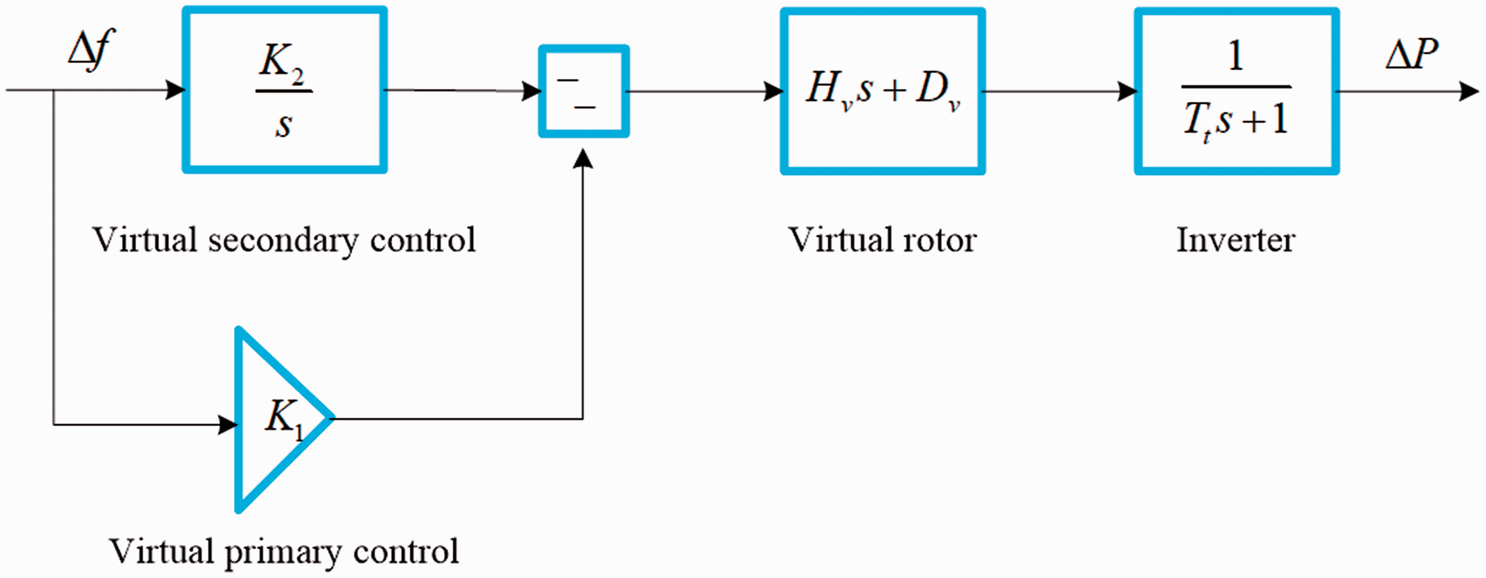
VSG model.

As revealed in Figure 1, it consists of four blocks, including virtual primary control, virtual secondary control, virtual rotor and inverter, where K₁ is the virtual main control coefficient, and K₂ is the virtual auxiliary control coefficient. The “virtual rotor” connected with the inverter is introduced to represent the damping and inertia characteristics of the power generator. In the model, K₁ and K₂ are the key factors in the frequency regulation and the control stability of the system. The relationship between the mechanical power change and load power change in the swing equation of a synchronous generator is as follows (Alipoor et al., 2015):

Δ P_{machine} - Δ P_{load} = (2 H s + D) Δ f

(1)

where

Δ P_{machine}

represents the mechanical power change;

Δ P_{load}

is the load power change; H is the system inertia coefficient; D represents the damping coefficient;

Δ f

is the power system frequency deviation.

The power reference value (P_r) of the inverter is obtained through the swing equation of the synchronous generator, as follows:

P_{r} = (H_{v} s + D_{v}) Δ f

(2)

where H_v is the virtual inertia coefficient, and D_v is the virtual damping coefficient. H_v and D_v are constant and used to simulate the inertia and damping characteristics of synchronous generator in the virtual rotor, respectively.

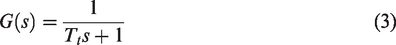
The first-order transfer function is used to model the inverter, expressed as follows:

G (s) = \frac{1}{T_{t} s + 1}

(3)

where T_t is a time constant with a small value.

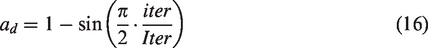
The primary frequency control and secondary frequency control in the synchronous generator were simulated using a PI controller as follows:

Δ P = (K_{1} + \frac{K_{2}}{s}) Δ f

(4)

where K₁ represents the primary frequency control gain; K₂ represents the second frequency control gain.

Virtual controller parameters optimization based on DGWO algorithm

Fundamental of GWO

GWO algorithm was proposed by Mirjalili et al. (2014). It simulates the behaviors of wolves in searching and hunting for food in nature environment. The wolves are divided into α wolf, β wolf, δ wolf and ω wolf according to the searching food capability. Wolves can cooperate with each other to complete the search process. α wolf is the leading wolf with an absolute dominant position, which is mainly responsible for food searching and hunting. β wolf is working under the leadership of α wolf and leads δ wolf and ω wolf. δ and ω wolves work at the lowest level, where they are subject to the leadership of α and β wolves.

The process of GWO algorithm is shown as follows (Mirjalili et al., 2016; Sulaiman et al., 2015):

First, the fitness value of the population is calculated, and the wolf pack is divided from the fitness values. Three wolves with the best fitness values are in order labeled as α wolf, β wolf and δ wolf, respectively. The remaining wolves are regarded as ω wolves.

The wolves begin to surround the prey after finding it. At this time, the gray wolf location is obtained as:

P (iter + 1) = P_{L} (iter) - A \cdot D

(5)

D = | G \cdot P_{L} (iter) - P (iter) |

(6)

where iter represents the current iteration number; P_L(iter) is the prey position; G(G = 2 v₁) indicates the swing coefficient; v₁ denotes the random number in the [0, 1] interval; A is the convergence coefficient and calculated as follows:

A = 2 a \cdot v_{2} - a

(7)

where v₂ is the random number in the [0, 1] interval; a is the convergence factor, which determines the value of A.

a = 2 \cdot (1 - \frac{iter}{Iter})

(8)

where Iter is the maximum number of iterations; a decreases linearly from 2 to 0.

(3) The wolves hunt the prey when α wolf finds it. At this time, the swing coefficients of α, β and δ wolves are updated as:

D_{α} = | G_{α} \cdot P_{α} (iter) - P (iter) |

(9)

D_{β} = | G_{β} \cdot P_{β} (iter) - P (iter) |

(10)

D_{δ} = | G_{δ} \cdot P_{δ} (iter) - P (iter) |

(11)

The positions of α, β and δ wolves are updated as follows:

P_{α} (iter + 1) = P_{α} (iter) - A_{α} D_{α}

(12)

P_{β} (iter + 1) = P_{β} (iter) - A_{β} D_{β}

(13)

P_{δ} (iter + 1) = P_{δ} (iter) - A_{δ} D_{δ}

(14)

The location of ω wolf is calculated as:

P_{ω} (iter + 1) = \frac{1}{3} (P_{α} (iter) + P_{β} (iter) + P_{δ} (iter))

(15)

The positions of α, β, δ and ω wolves are depicted in Figure 2.

Figure 2.

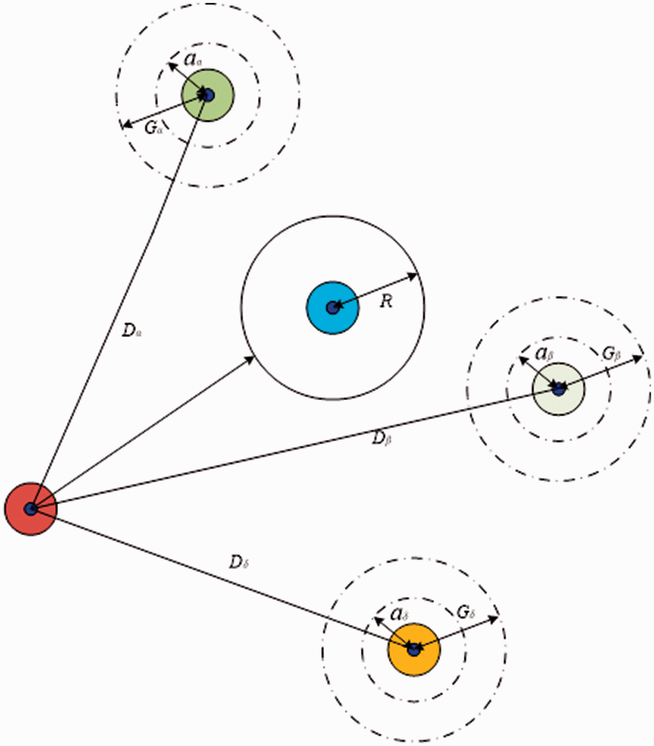
Gray wolf location.

Selection of convergence factor in GWO algorithm

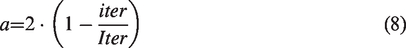
The wolves search and surround the prey by adjusting the convergence coefficient A in the GWO algorithm. The value of A is determined by the convergence factor a, where a decreases linearly from 2 to 0; the interval of A is [−2a, 2a]. In practice, the linear convergence factor a cannot balance local and global search abilities concurrently. Therefore, the dynamic convergence factor a_d is introduced to reach the target balance between the local and global searches.

a_{d} = 1 - \sin (\frac{π}{2} \cdot \frac{iter}{Iter})

(16)

where iter represents the current number of iterations, and Iter is the maximum number of iterations.

The convergence coefficient A based on the dynamic convergence factor is obtained as follows:

A = 2 a_{d} \cdot v_{2} - a_{d}

(17)

The curves of the linear and dynamic convergence factors over the number of iterations are shown in Figure 3.

Figure 3.

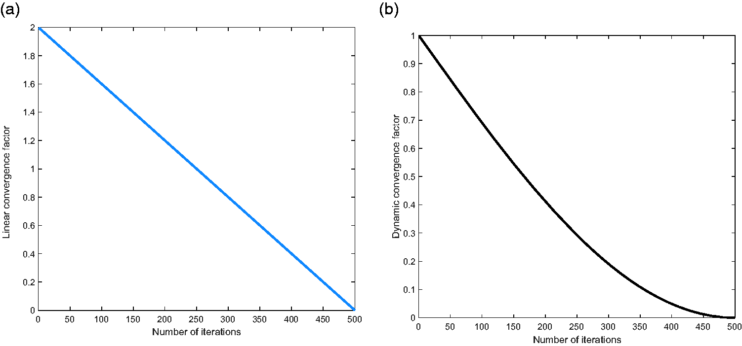
Convergence factor over iterations in GWO. (a) Linear convergence factor, (b) Dynamic convergence factor.

During 500 iterations, a converges to 0 linearly, as shown in Figure 3(a). Figure 3(b) shows that a_d decreases linearly before 250 iterations; after 250 iterations, a_d decreases nonlinearly. The linear and nonlinear variations in a_d were used to enhance the convergence performance of the GWO. Indeed, before 250 iterations, a_d leads to a global search to find the prey location; after 250 iterations, the a_d convergence speed is accelerated; at this time, it is focused on a local search.

On the other hand, the population diversity may decrease in the later stage of GWO iteration, especially for individuals with poor fitness, which can easily fall into a local optimum. The random walk characteristic of the Levy flight makes GWO have a stronger global search ability. Therefore, this study uses the Levy mutation to prevent the ω wolf from prematurely falling into extreme values.

Levy flight has strong randomness and variability in long-distance jumping situations. The random walk characteristics of the flight path are presented in Figure 4.

Figure 4.

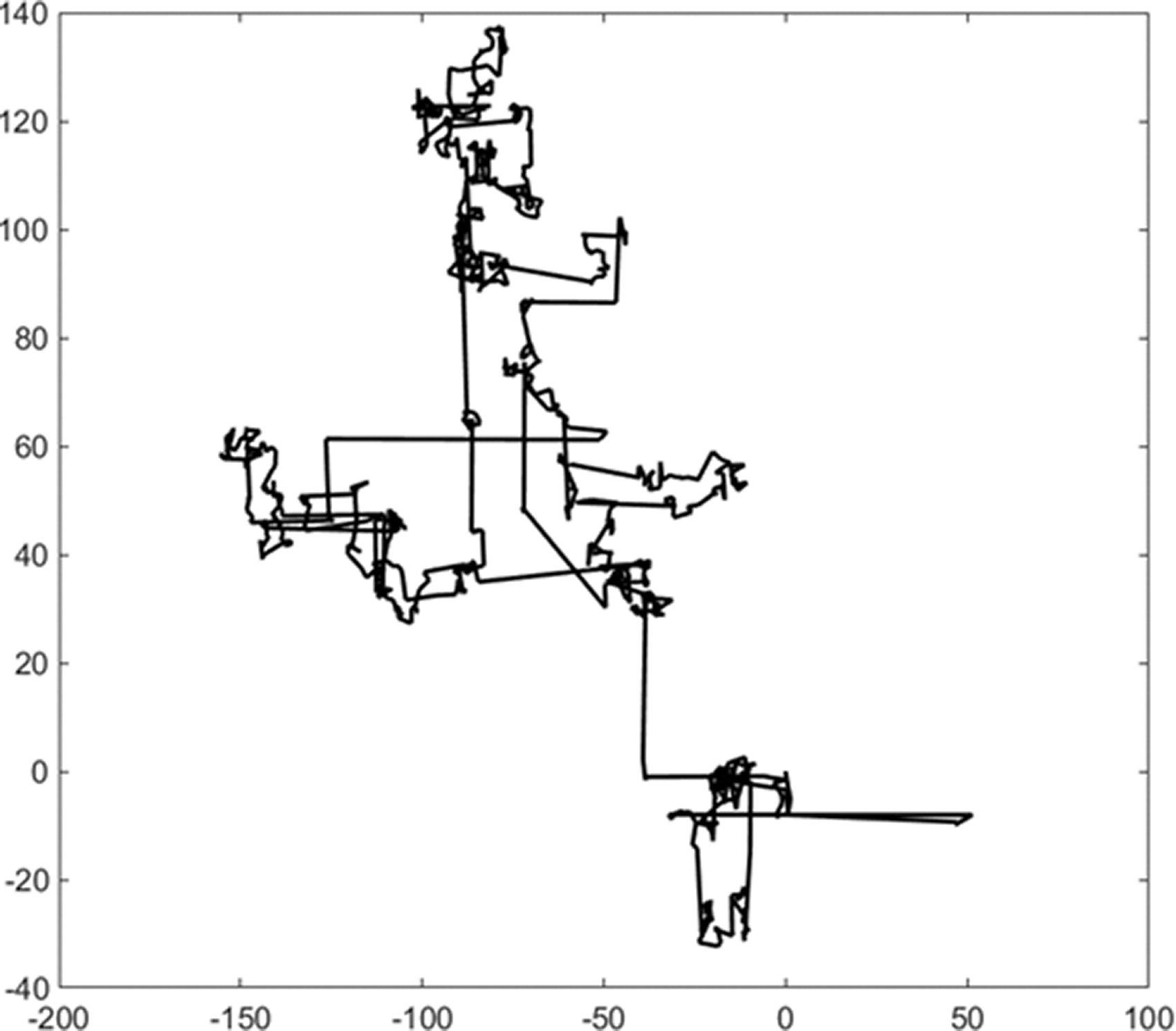
Levy flight path.

Levy's random walk feature was applied to improve the population diversity in the later stages of the GWO algorithm. Its flight path is expressed as follows (Edwards et al., 2007):

Levy \sim \frac{u}{{| e |}^{\frac{1}{γ}}}

(18)

where γ (1 <γ < 3); u(u∼N(0, σ_u²)) and e(e∼N(0, σ_e²)) obey a normal distribution; σ_u and σ_e are calculated as follows (Barthelemy et al., 2008):

{\begin{array}{l} σ_{u} = {[\frac{Γ (1 + γ) \cdot \sin (\frac{γ}{2} π)}{Γ (\frac{1 + γ}{2}) \cdot γ \cdot 2^{\frac{1 + γ}{2}})}]}^{\frac{1}{γ}} \\ σ_{e} = 1 \end{array}

(19)

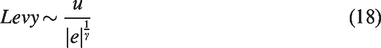
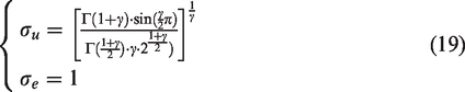
During the iteration process, the DGWO algorithm easily falls into a local optimal value and is unlikely to reach the global optimization solution. By making use of the random walk characteristics of Levy flight, the DGWO algorithm can maintain a strong global search performance in the later iteration period, thus achieving better convergence results.

After Levy flight is introduced into the ω wolf, the gray wolf location can be found, expressed as follows:

P_{ω} (iter + 1) = P_{ω} (iter + 1) + Levy \otimes P_{ω} (iter)

(20)

Validation of the proposed DGWO algorithm

The nonlinear convergence factor and Levy mutation are integrated to ensure the balance of search ability and population diversity in the DGWO algorithm. Unimodal and multimodal functions are used to evaluate the algorithm performance efficiency. Unimodal test functions have one global optimal point without extremum points. Multimodal functions have multiple extremum points in addition to a global optimum. Accordingly, unimodal functions are used to test the global optimization ability, and the multimodal function are used to test the ability of escaping from local extremes. Two unimodal functions (F₁ and F₂) and three multimodal functions (F₃, F₄ and F₅) are employed to analyze the convergence effect, as shown in Table 1.

Table 1.

Unimodal and multimodal test functions (Li et al., 2020, 2021).

Functions	Dim	Variable range	Property
$F_{1} = \sum_{i = 1}^{Dim} υ_{i}^{2}$	50	[–1,00,100]	Unimodality
$F_{2} = \sum_{i = 1}^{Dim} \| υ_{i}^{} \| + \prod_{i = 1}^{Dim} \| υ_{i}^{} \|$	50	[–10, 10]	Unimodality
$F_{3} = \sum_{i = 1}^{Dim} υ_{i}^{2} - 10 \cdot \cos (2 π υ_{i}) + 10 \cdot Dim$	50	[–5.12, 5.12]	Multimodality
$\begin{array}{l} F_{4} = 20 - 20 \cdot \exp (- 0.2 \sqrt{\frac{1}{Dim} \sum_{i = 1}^{Dim} υ_{i}^{2}}) \dots \\ - \exp (\frac{1}{Dim} \cos (2 π υ_{i})) + \exp (1) \end{array}$	50	[–32, 32]	Multimodality
$F_{5} = \frac{1}{4000} \sum_{i = 1}^{Dim} υ_{i}^{2} - \prod_{i = 1}^{Dim} \cos (\frac{υ_{i}}{\sqrt{i}}) + 1$	50	[–6,00,600]	Multimodality

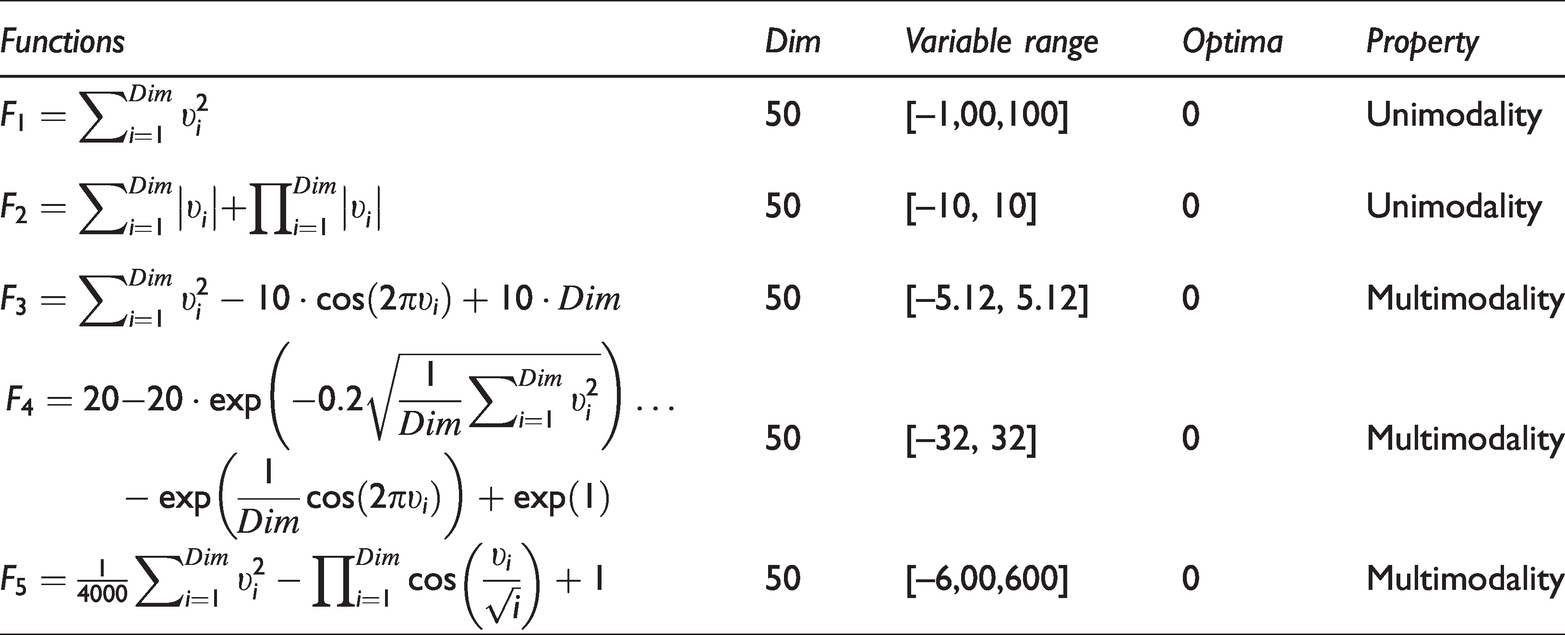
The testing dimensions of the five standard test functions are unified to 50, and the global optimal values are all set as 0. Whale Optimization Algorithm (WOA), Particle Swarm Optimization Algorithm (PSO) (Van den Bergh and Engelbrecht, 2004), GWO algorithm and the DGWO algorithm were tested for comparison. The parameter settings of these algorithms are listed in Table 2.

Table 2.

Parameters setting in optimization process.

Algorithm	Parameters
PSO	w_max=0.9, w_min=0.1, c₁=c₂=1.494, pop = 30, Iter = 500
WOA	b = 1, pop = 30, Iter = 500
GWO	pop = 30, Iter = 500
DGWO	pop = 30, Iter = 500

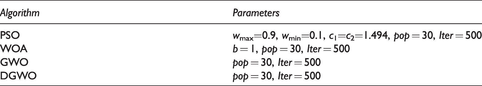
The maximum number of iterations and population size in four algorithms are set under the same values, where the maximum number of iterations is 500 and the population size is 30. For PSO algorithm, w_max and w_min represent the maximum and minimum weights, respectively; c₁ and c₂ denote the self-learning and social learning abilities, respectively. For the WOA algorithm, the spiral coefficient b is set as 1. As above, GWO and DGWO have less adjustable parameters number compared with PSO and WOA algorithms.

The convergence performance is evaluated using worst convergence value, optimal convergence value, mean convergence value, and standard deviation (std) under 30 repeated runs. The convergence test results are concluded in Table 3.

Table 3.

Convergence test results.

F	Algorithm	Worst convergence value	Optimal convergence value	Mean convergence value	std
F ₁	PSO	899.78	83.90	341.77	183.09
	WOA	9.81E-72	2.90E-86	3.42E-73	1.78E-72
	GWO	9.70E-19	2.96E-21	9.48E-20	2.15E-19
	DGWO	0	0	0	0
F ₂	PSO	23.06	4.06	11.29	4.06
	WOA	1.08E-48	2.02E-57	4.62E-50	1.96E-49
	GWO	5.50E-12	8.13E-13	2.43E-12	1.46E-12
	DGWO	7.71E-189	9.64E-192	8.34E-190	0
F ₃	PSO	97.72	30.36	54.32	14.95
	WOA	0	0	0	0
	GWO	21.58	1.13E-13	5.49	5.47
	DGWO	0	0	0	0
F ₄	PSO	11.78	4.42	7.94	1.99
	WOA	7.99E-15	8.88E-16	4.20E-15	2.62E-15
	GWO	9.95E-11	1.05E-11	4.02E-11	2.57E-11
	DGWO	4.44E-15	8.88E-16	1.48E-15	1.34E-15
F ₅	PSO	7.21	1.26	3.80	1.51
	WOA	0.21	0	7.1E-03	3.87E-02
	GWO	3.11E-02	0	4.7E-03	9.1E-03
	DGWO	0	0	0	0

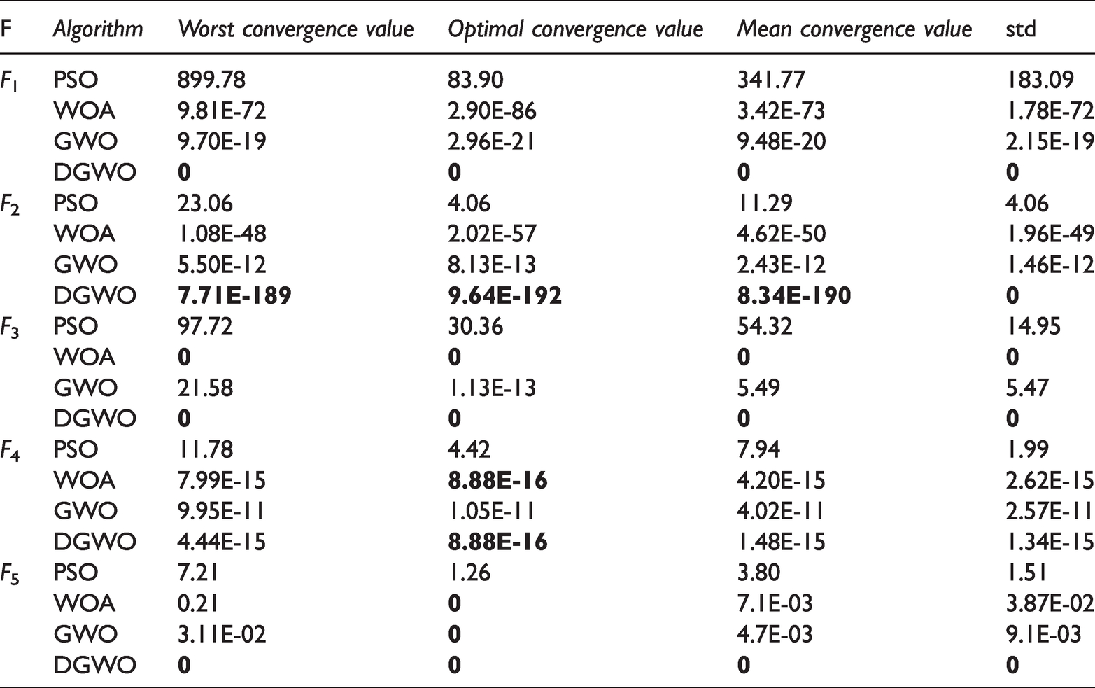
It is clear that DGWO algorithm provides most satisfactory results from F₁ to F₅, particularly convergence value equal to 0 in F₁, F₃ and F₅. Although the convergence values of GWO and WOA algorithms can reach 0 in F₃ and F₅ in some convergence values, they do not achieve 0 in all values. On the contrary, PSO algorithm has worse convergence value in general, e.g. up to 23.06 in F₂, due to the lack of dynamic speed adjustment.

The convergence curves using GWO and DGWO algorithms from F₁ to F₅ tests are shown in Figure 5.

Figure 5.

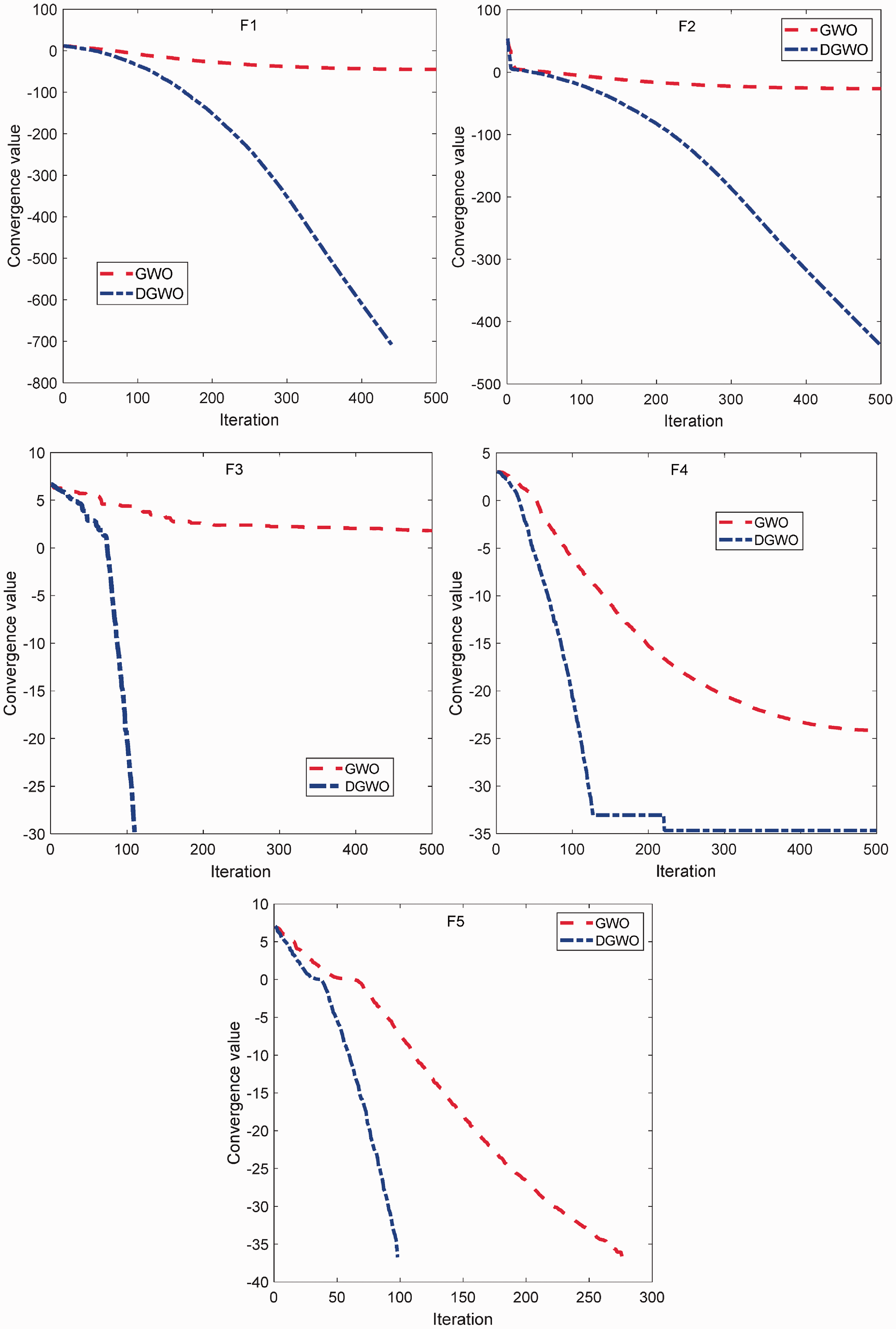
Convergence curves in GWO and DGWO algorithms.

As can be seen, the DGWO algorithm has larger convergence slope from F₁ to F₅ test, and it indicates a faster convergence rate compared with GWO algorithm. For example, the convergence value of DGWO algorithm in F₅ test reaches 0 within around 100 iterations, but the GWO algorithm requires around 280 iterations.

Parameters optimization process in virtual controller

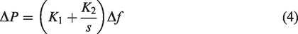
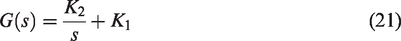
The VSG can simulate the inertial response of the synchronous generator through the signal sent by virtual controller. The virtual control is realized through the proportional gain K₁ and the integral gain K₂ in the VSG model. The system inertia and the system frequency can be stabilized by adjusting K₁ and K₂. The transfer function of the virtual controller is expressed as follows:

G (s) = \frac{K_{2}}{s} + K_{1}

(21)

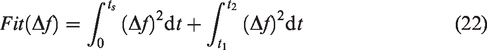
The DGWO algorithm is introduced to select appropriate K₁ and K₂ based on the parameters optimization process. The square of the frequency deviation is defined as the fitness function to evaluate the system frequency deviation, shown as below:

Fit (Δ f) = \int_{0}^{t_{s}} {(Δ f)}^{2} d t + \int_{t_{1}}^{t_{2}} {(Δ f)}^{2} d t

(22)

where t_s represents the simulation time; t₁ and t₂ are the start time and stop time of the system during the transient operation, respectively. Note that both steady state and transient state in the system frequency deviation are taken account in realization simultaneously.

Performance simulation and analysis

High permeability renewable energy grid modeling

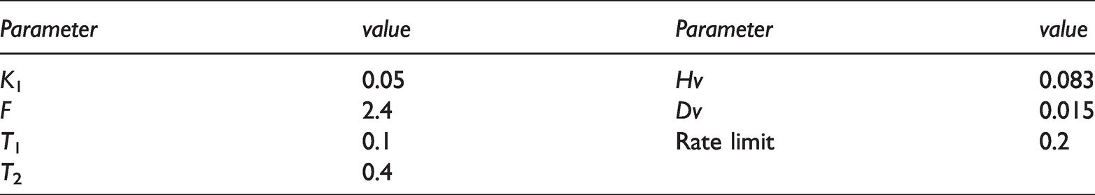
A high permeability renewable energy grid system is considered in the proposed VSG control strategy. It includes photovoltaic power generation system, wind power generation system, traditional thermal power generation system and electric load. Among them, the generation and governor dead zone constraints are used to simulate the nonlinear constraints of the generator set. The renewable energy grid system with virtual synchronous machine control is depicted in Figure 6, and the major parameters of renewable energy grid system are listed in Table 4.

Figure 6.

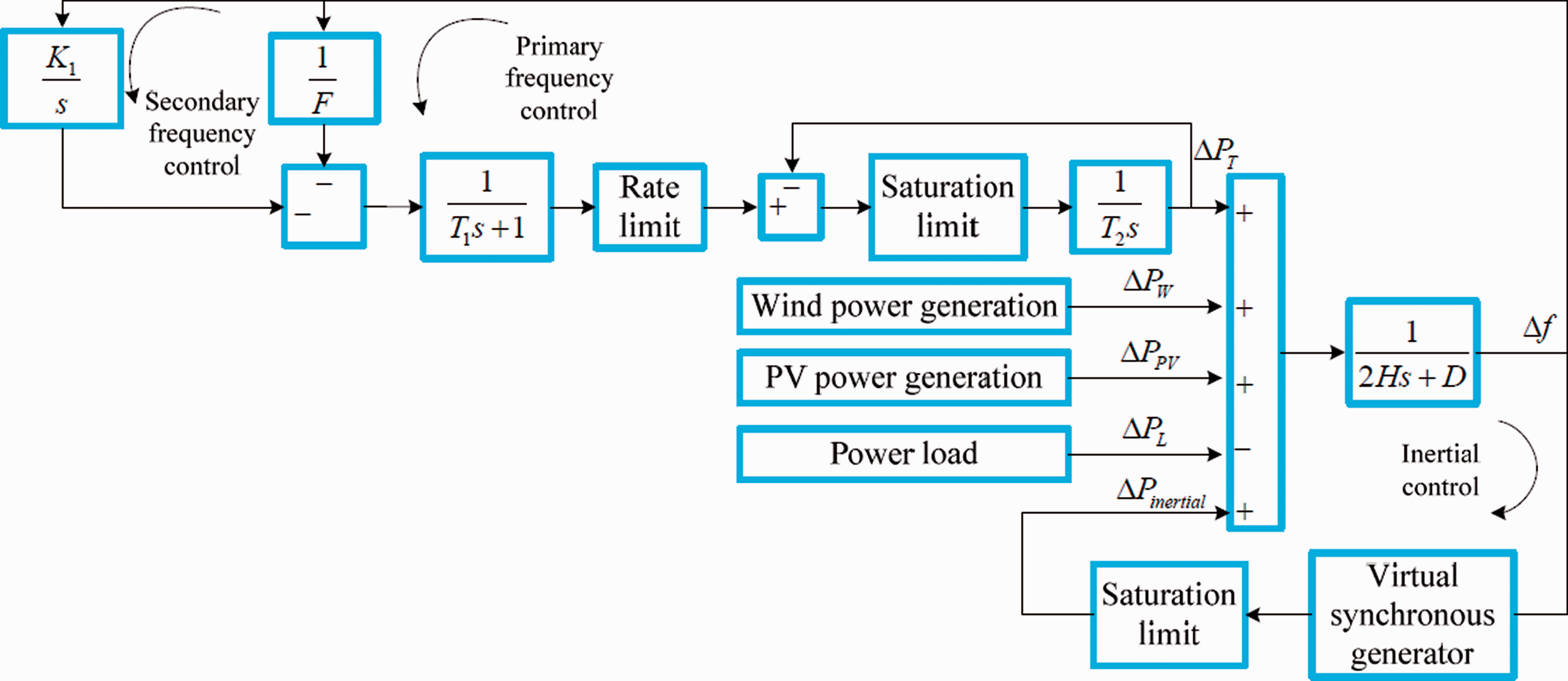
Renewable energy grid system with virtual synchronous machine control.

Table 4.

Parameters of high permeability energy grid system (Magdy et al., 2019).

Parameter	value	Parameter	value
K ₁	0.05	Hv	0.083
F	2.4	Dv	0.015
T ₁	0.1	Rate limit	0.2
T ₂	0.4

As shown in Figure 6, the renewable energy grid system is built using the MATLAB/Simulink simulation platform. It includes 5 MW solar power generation, 10 MW wind power generation, 15 MW power load and 20 MW thermal power generation. Simultaneously, the inherent nonlinear requirements in the system are considered and expressed by the saturation limit model.

Wind power generation model

The wind power is generated by random wind speed on the basis of the rated wind speed and the white noise signal in the Matlab simulation module. The specific wind power model is depicted in Figure 7.

Figure 7.

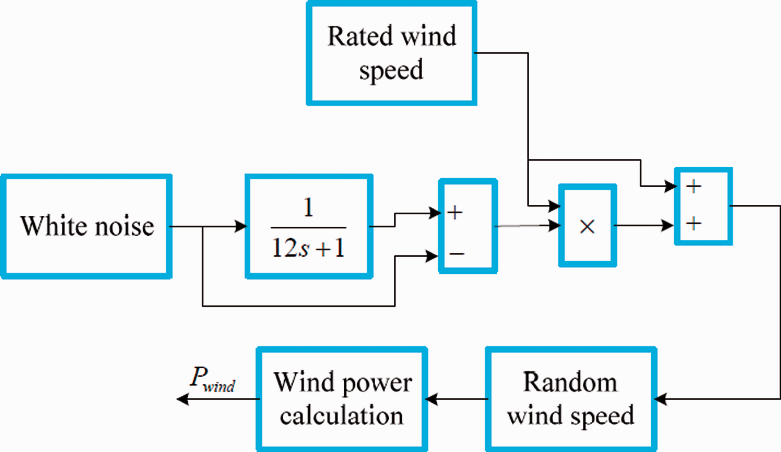
Wind power model.

As revealed in Figure 7, when the random wind speed is obtained, the wind power is calculated as follows:

P_{wind} = 0.5 \cdot C (λ, ε) \cdot d_{air} \cdot A_{r} \cdot W_{speed}^{3}

(23)

where d_air(=1.23) denotes the air density; A_r(=5905) represents the reduced area of the rotor; W_speed(=12) is the wind speed; C(λ, ε) is the power conversion coefficient. The mathematical model is expressed as follows:

C (λ, ε) = h_{1} \cdot \exp (- \frac{h_{2}}{o_{1}}) \cdot (\frac{h_{3}}{o_{1}} - h_{4} ε - h_{5} ε^{2} - h_{6}) + h_{7} o_{2}

(24)

where o₁ is the intermittent best tip speed ratio; o₂ is the best tip speed ratio; h(h₁=0.39; h₂=116; h₃=0.40; h₄=0.42; h₅=21; h₆=0.02) represents the turbine coefficient; ε is the pitch angle.

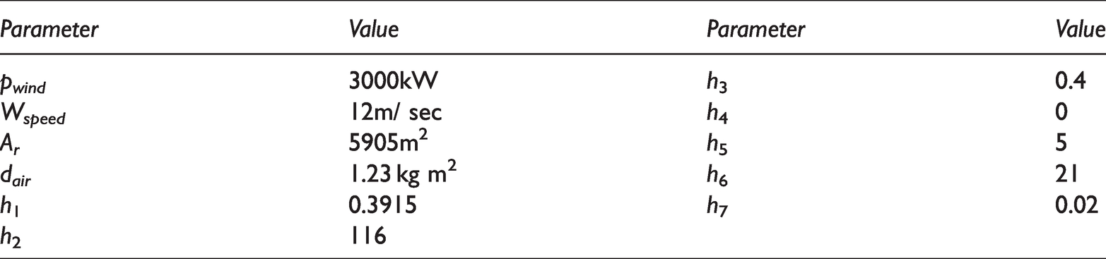
The wind turbine parameters are listed in Table 5.

Table 5.

Wind turbine parameters.

Parameter	Value	Parameter	Value
p_wind	3000kW	h ₃	0.4
W_speed	12m/ sec	h ₄	0
A_r	5905m²	h ₅	5
d_air	1.23 kg m²	h ₆	21
h ₁	0.3915	h ₇	0.02
h ₂	116

The wind power generation distribution depicted in Figure 8 is produced from equation (23) based on the wind power model in Figure 7. It indicates that the wind power has strong nonlinearity and volatility characteristics.

Figure 8.

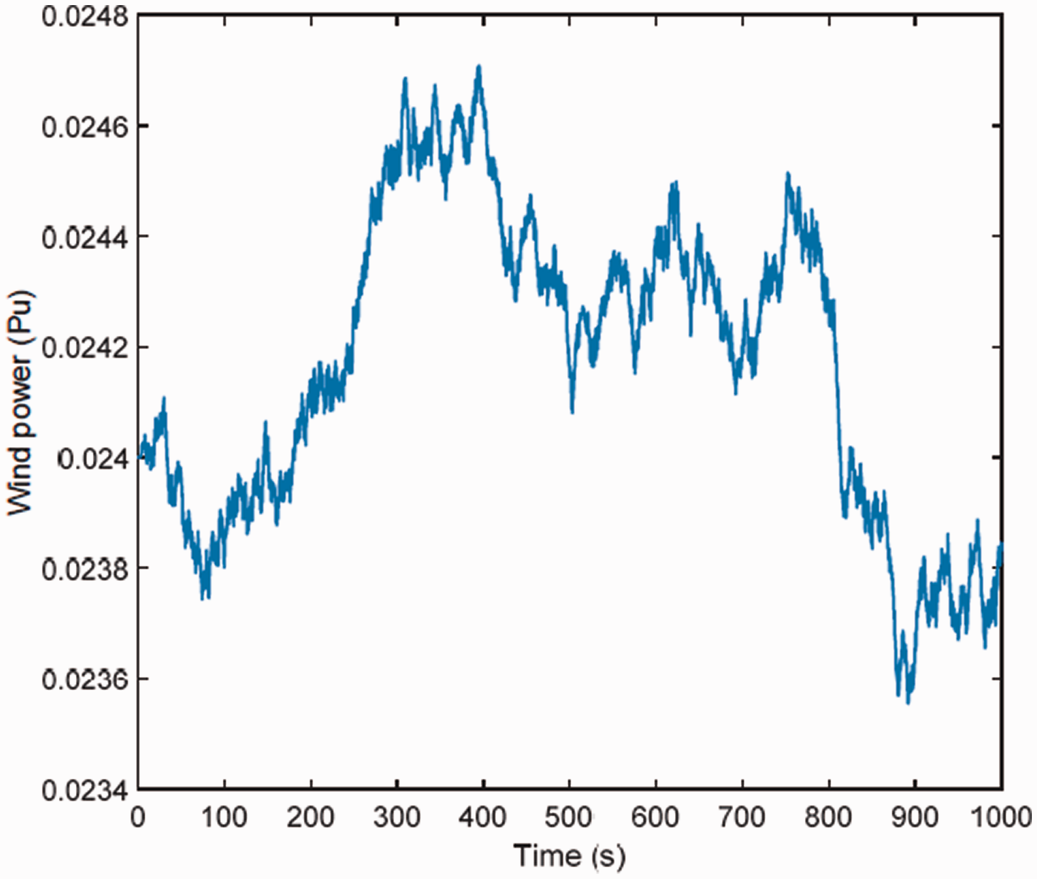
Wind power generation distribution.

Photovoltaic power generation model

The rated power of photovoltaic power generation is equivalent to the sum of the rated power values of each photovoltaic unit. In an actual situation, the photovoltaic power generation has randomness depending on a weather condition. For this reason, it is simulated through the white noise signal and the standard deviation using the Matlab simulation module. The photovoltaic power generation model is shown in Figure 9.

Figure 9.

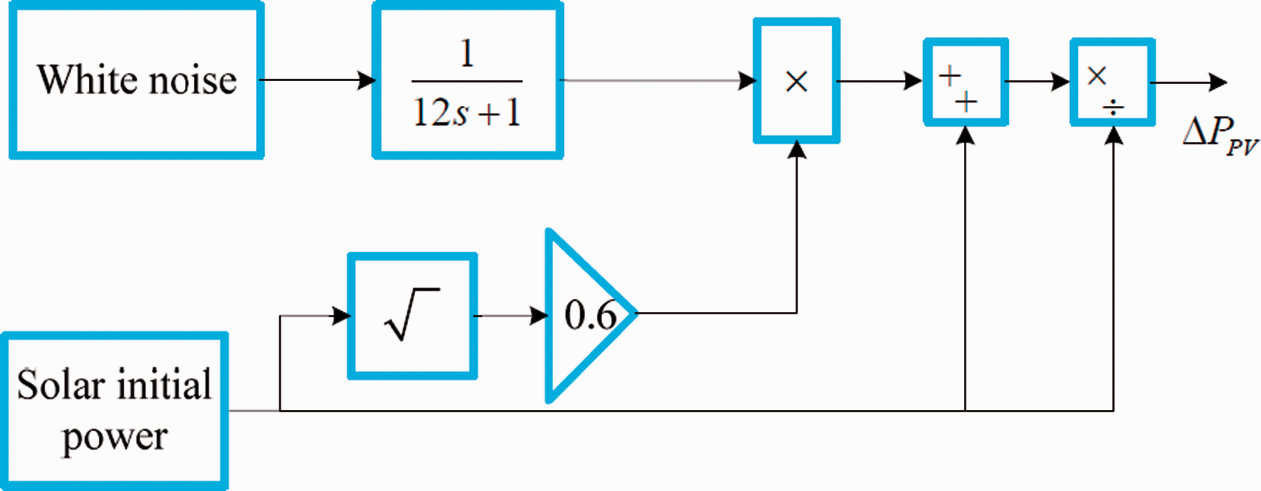
Photovoltaic power model.

The PV power deviation is expressed as follows:

Δ P_{P V} = 0.6 \sqrt{P_{P V}}

(25)

Based on the PV photovoltaic power model in Figure 9, the PV power generation distribution is shown in Figure 10. Similarly, the power curve reveals strong randomness and volatility.

Figure 10.

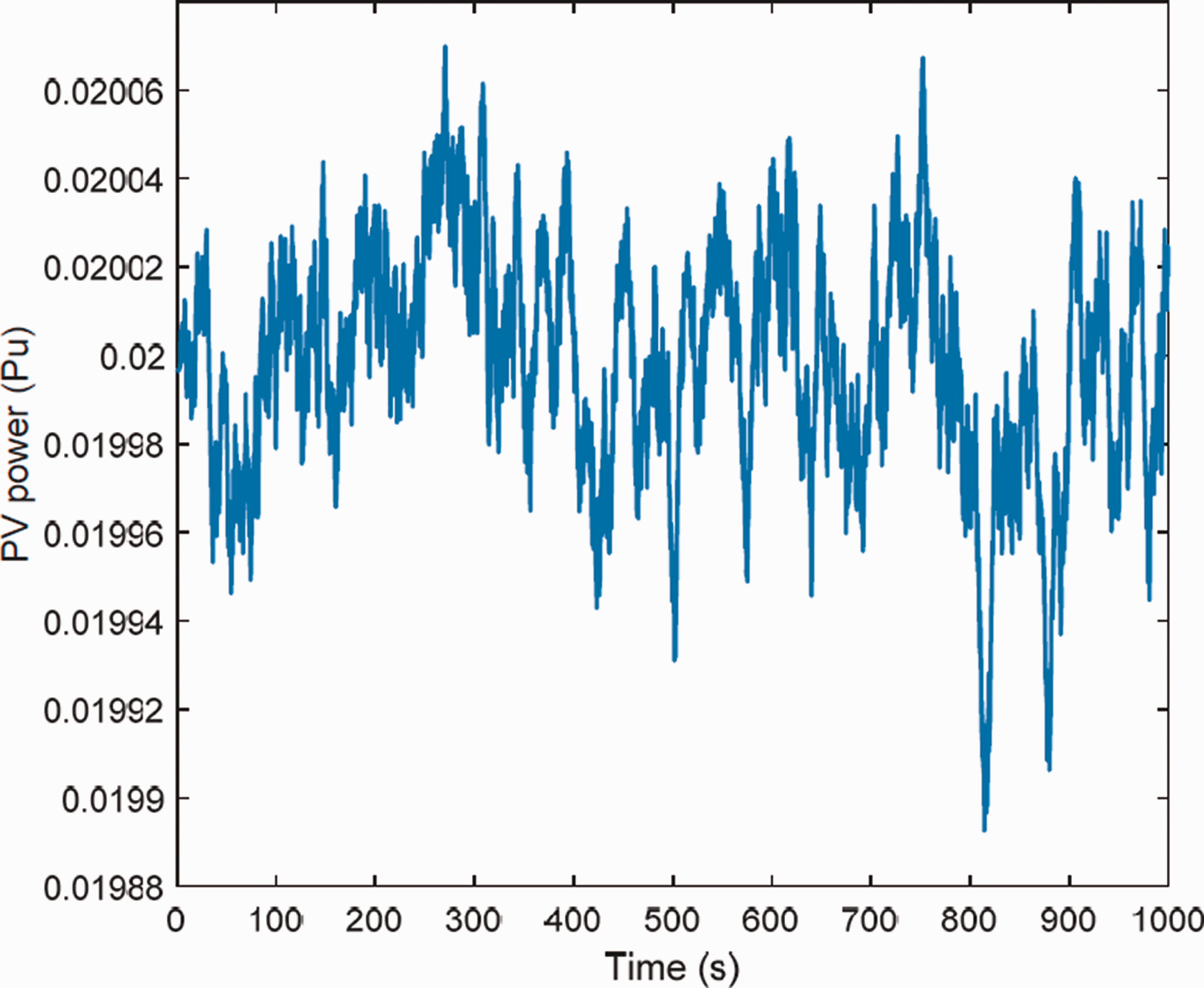
PV power generation distribution.

Power load model

In reality, there are various non-linear loads utilized in the power line. For this reason, the white noise signal multiplying the initial load deviation is used to simulate the electric power load in the Matlab simulation module, as shown in Figure 11.

Figure 11.

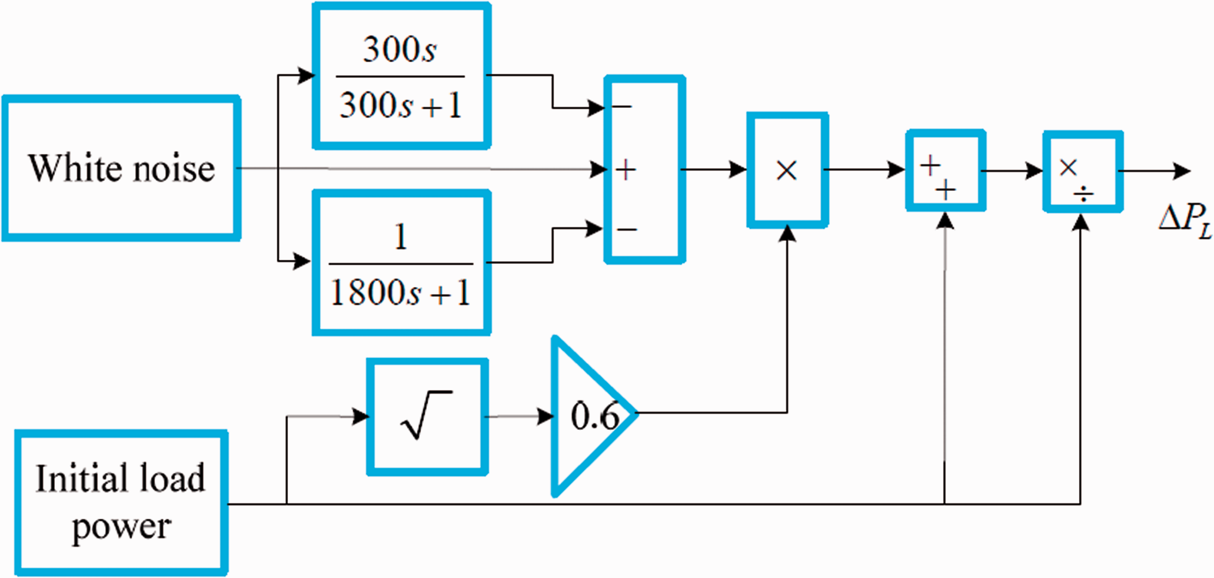
Power load model.

Load deviation to simulate the actual load variation is expressed as

Δ P_{L} = 0.6 \sqrt{P_{load}}

(26)

The random load power is simulated based on the power load model from Figure 11, and its result is shown in Figure 12. In this model, the load power contains white noise signal so that it can represent possible real circumstance with strong randomness.

Figure 12.

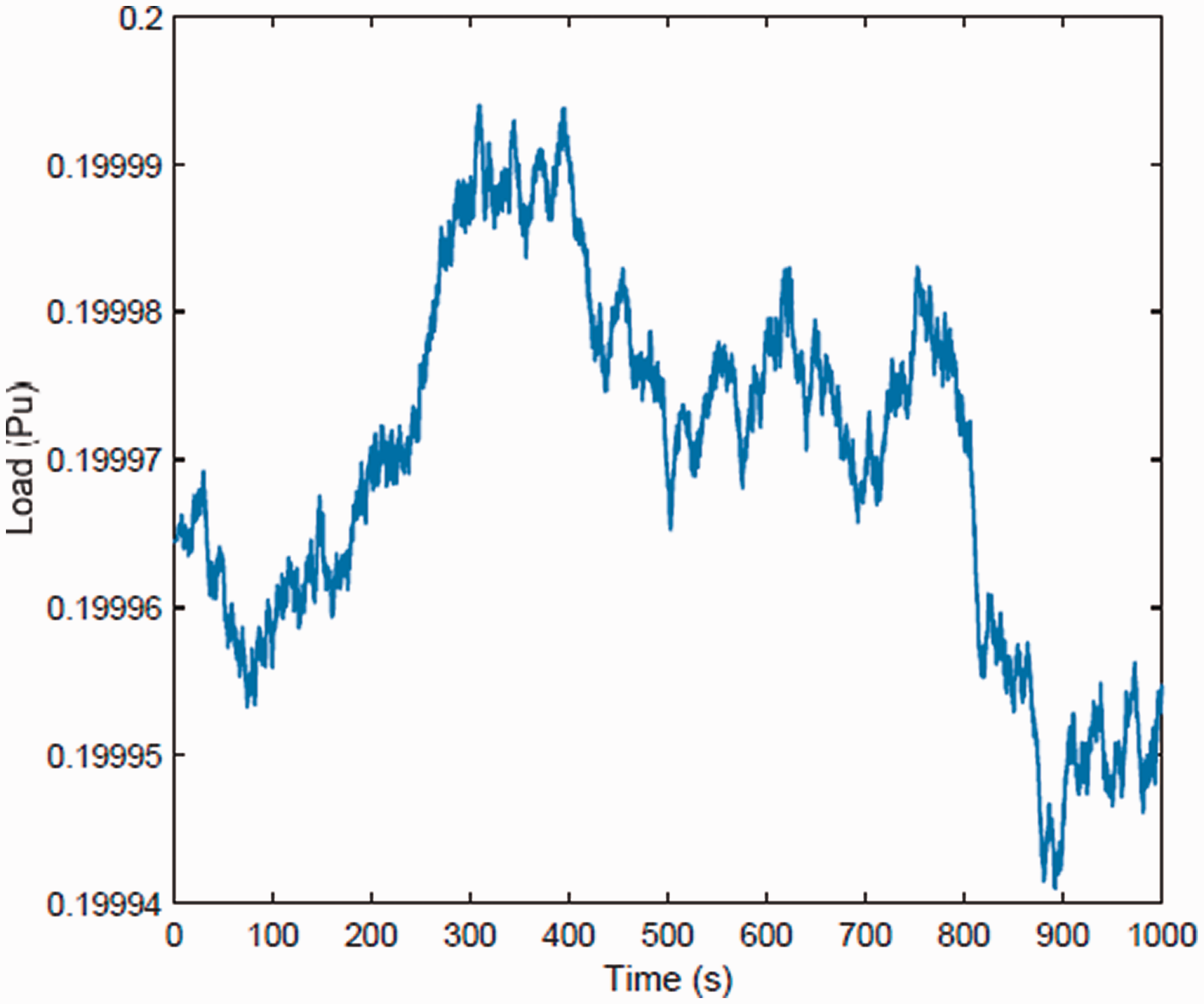
Random load power.

Validation of the proposed virtual inertial control strategy

Performance test under step load disturbance

The overall schematic process in optimizing virtual control parameters in the DGWO algorithm is illustrated in Figure 13.

Figure 13.

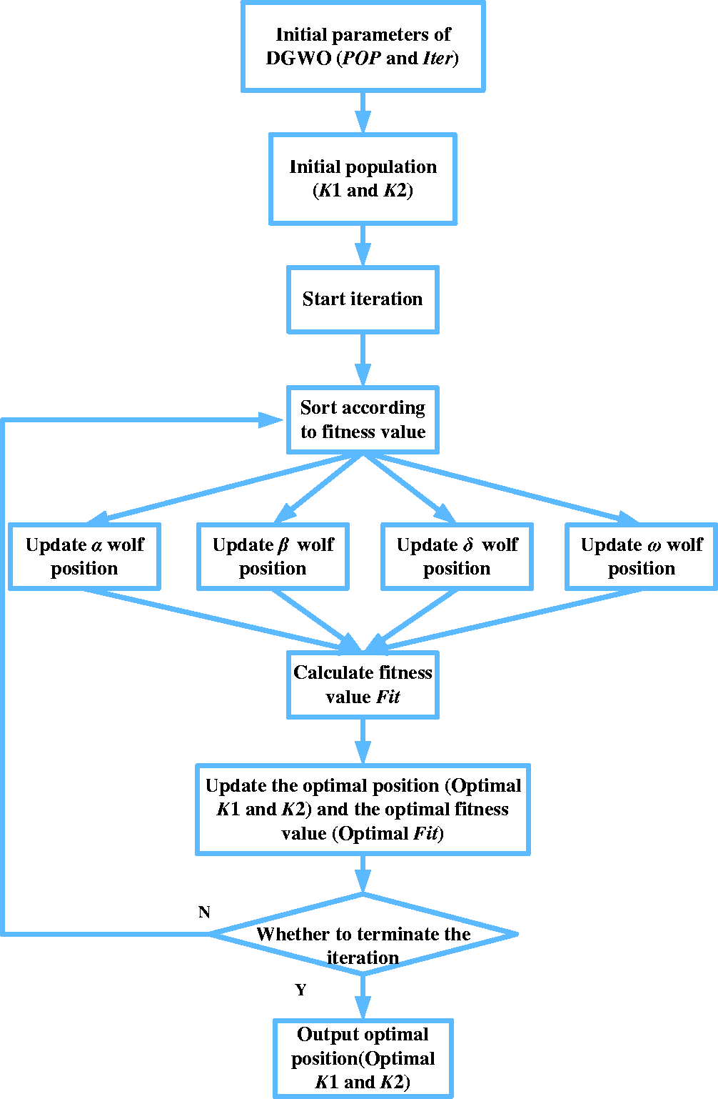
Parameters optimization process of virtual controller.

Figure 13 depicts the virtual controller parameter optimization process on the basis of the DGWO algorithm, including the following aspects:

Initialize the DGWO algorithm parameters, such as population size and number of iterations;

Initialize the population (K₁ and K₂) and calculate the fitness value (Fit);

Start to optimize virtual controller parameters;

Sort the wolves according to the fitness value;

Update the positions of α, β and δ wolves;

Determine whether to mutate ω wolf, if necessary. Use Levy mutation strategy to update the position of ω wolf. Otherwise, keep the original position;

Calculate the fitness values of α, β, δ and ω wolves;

Update the optimal position;

Determine whether to terminate the iteration when the condition of iteration termination is met. Otherwise, return to the fourth step;

Output the optimal parameters K₁ and K₂ of the virtual controller.

The Matlab/Simulink R2019a module is used to validate the proposed method. First, the simulation performance was carried out under a low inertia system (30% of its nominal value). The proposed method is tested under step load and random load. The amplitude of step load does not change with time, while the amplitude of random load varies with time. The step load is added to simulate the influence of sudden generator shutdown or random load increase in the power system. The performance period time is 1000 s, and 0.05pu step load is added at t = 600s. The comparison between traditional and proposed control strategies is revealed in Figure 14.

Figure 14.

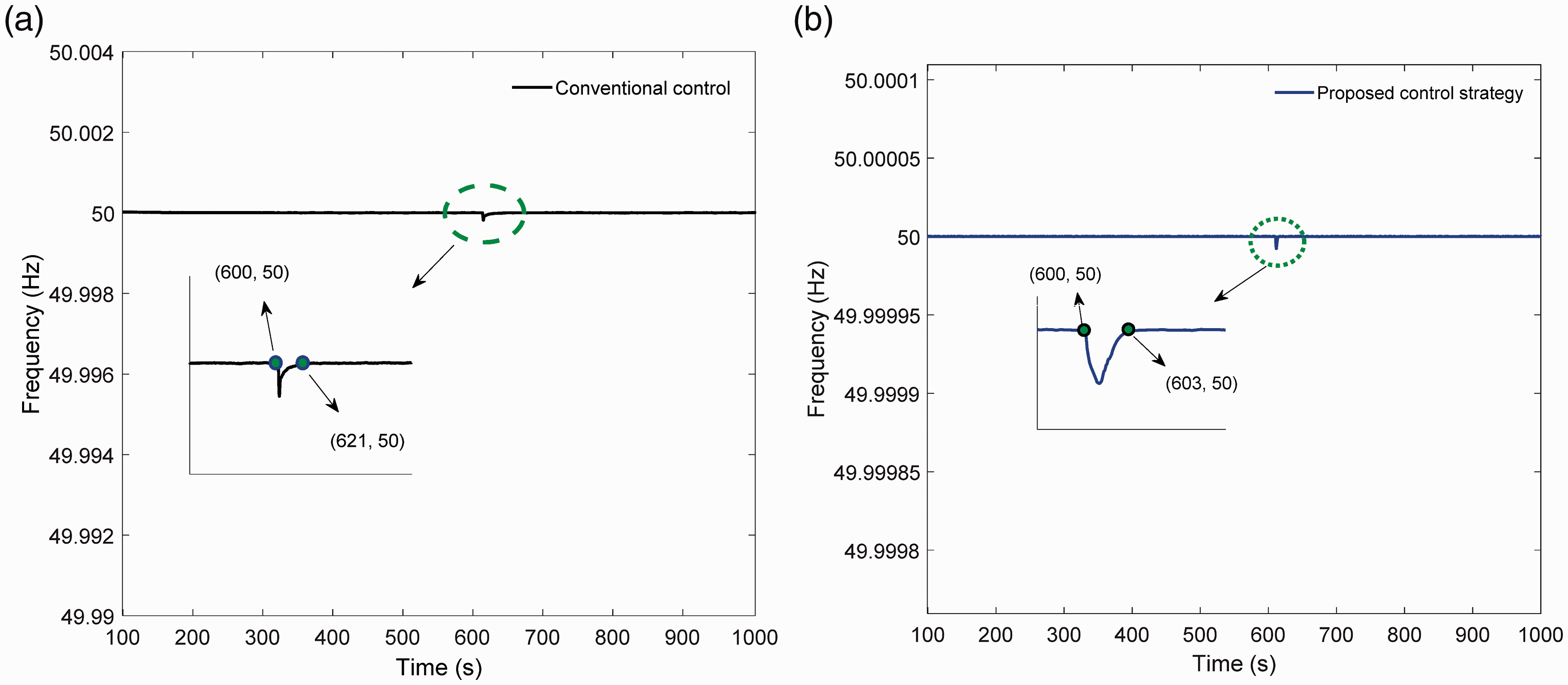
Test results under step load. (a) Conventional control, (b) Proposed control strategy.

In Figure 14(a), the power system frequency begins to drop at t = 600s. For traditional control, it is found that 21 s was demanded for the system to recover from the frequency disturbance point back to the frequency stability point. In contrast, it only requires 3 s for the system returning to normal by the proposed control strategy. It is obvious that the frequency fluctuation in Figure 14(a) is greater than that in Figure 14(b) when the step load is added. It shows that the proposed control strategy has better stability in system frequency. Moreover, the inverter in the virtual controller has an inertial effect so that the system frequency can drop more slowly than traditional one.

Performance test under random load disturbance

In the test using the random load (as depicted in Figure 12), the power system frequency begins to drop at t = 600s during 1000 s period time. The results from traditional and the proposed control methods are revealed in Figure 15.

Figure 15.

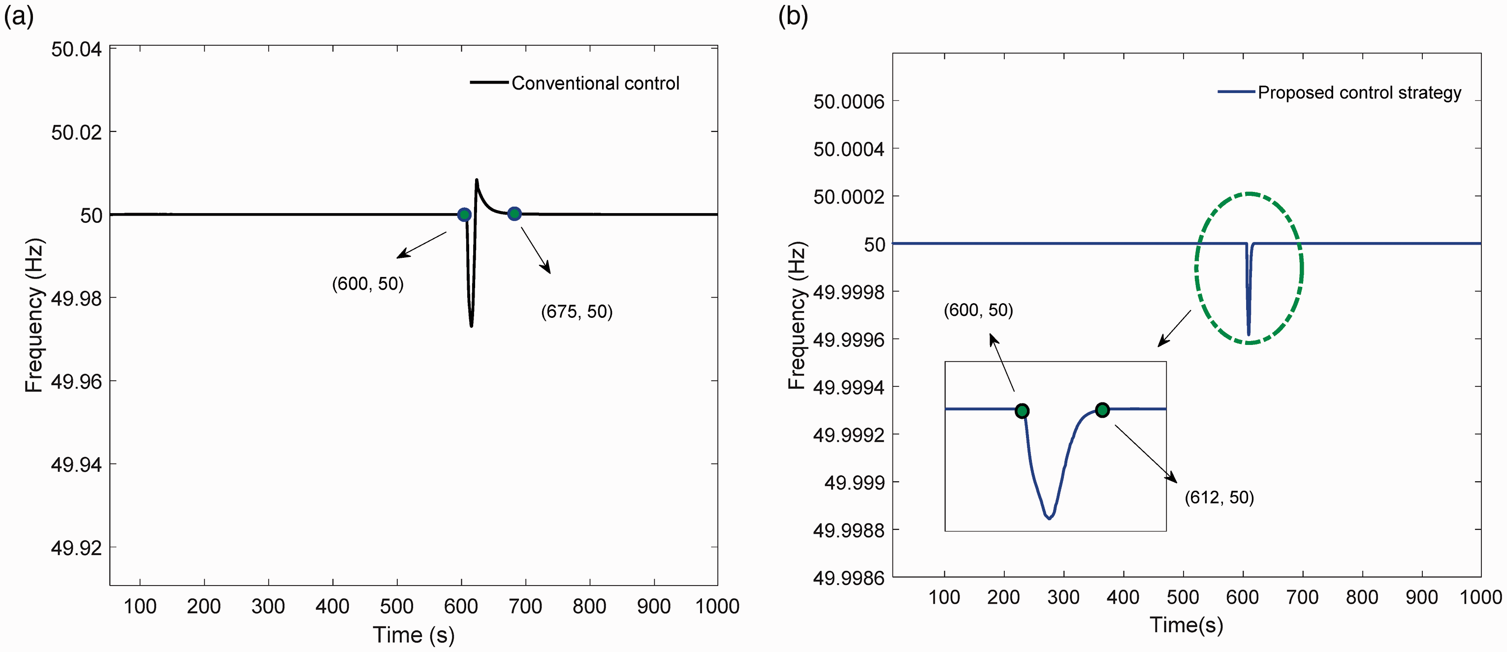
Test results using random load. (a) Conventional control, (b) Proposed control strategy.

From the test results as above, the frequency fluctuations of both control methods are greater than the step load, and longer time is needed to return to a stable state. It indicates that 75 s is taken for the system frequency to recover from the fluctuation point to the stable point in the traditional control method. In the proposed virtual control strategy, only 12 s is required for the system frequency returning to normal. Besides, it is clear that the frequency changing slope from t = 600s is considerably lower than the conventional one.

Through the above analysis, it is found that the frequency regulation of the system is sensitive to parameters K₁ and K₂. In two load cases study, it is confirmed that the fluctuation of system frequency can be sufficiently stabilized in a shorter time. It implies that the sensitivity of system frequency regulation to parameters K₁ and K₂ can be reduced efficiently through parameter optimization process.

Conclusions

The high penetration level generated from renewable energy generation can reduce the power system inertia, affecting the system stability in a large-scale grid. Accordingly, the proposed virtual inertia control strategy can stabilize the system frequency in less time under a distinct power system fluctuation.

The main contributions in this study are concluded as follows:

The DGWO algorithm has been proven to present stronger local and global search balance ability than the GWO algorithm.

The convergence effect from DGWO algorithm is verified using unimodal and multimodal functions.

The crucial parameters such as K1 and K2 in the virtual synchronous VSM controller can be optimized based on the DGWO algorithm.

A feasible solution for stabilizing the system frequency and increasing the renewable energy permeability can be realized using the proposed control strategy.

Moreover, this study reveals that the operation time required to restore the system frequency to a stable condition takes 18 s and 63 s for step load and random load, respectively, indicating significantly less time than the traditional control algorithms. Future studies should focus on the generalization ability of multiple microgrid systems under a variety of renewable power sources.

Footnotes

Declaration of conflicting interests

The author(s) declared no potential conflicts of interest with respect to the research, authorship, and/or publication of this article.

Funding

The author(s) received no financial support for the research, authorship, and/or publication of this article.

ORCID iD

Hsiung-Cheng Lin

References

Abdollahi

Candela

Rocabert

, et al. (2020) Novel analytical method for dynamic design of renewable SSG SPC unit to mitigate low-frequency electromechanical oscillations. IEEE Transactions on Power Electronics 35(7): 7532–7544.

Alayi

Jahanbin

(2020) Generation management analysis of a stand-alone photovoltaic system with battery. Renewable Energy Research and Application 1(2): 205–209.

Ali

Magdy

, et al. (2019) A new frequency control strategy in an islanded microgrid using virtual inertia control-based coefficient diagram method. IEEE Access 7: 16979–16990.

Alipoor

Miura

Ise

(2015) Power system stabilization using virtual synchronous generator with alternating moment of inertia. IEEE Journal of Emerging and Selected Topics in Power Electronics 3(2): 451–458.

Alipoor

Miura

Ise

(2018) Stability assessment and optimization methods for microgrid with multiple VSG units. IEEE Transactions on Smart Grid 9(2): 1462–1471.

Al-Tameemi

Miura

Liu

(2020) A novel control scheme for multi-terminal low-frequency AC electrical energy transmission systems using modular multilevel matrix converters and virtual synchronous generator concept. Energies 13(3): 19.

Barthelemy

Bertolotti

Wiersma

(2008) A levy flight for light. Nature 453(7194): 495–498.

Bevrani

Ise

Miura

(2014) Virtual synchronous generators: A survey and new perspectives. International Journal of Electrical Power & Energy Systems 54: 244–254.

Chen

Liu

Milano

(2020) 100% Converter-interfaced generation using virtual synchronous generator control: A case study based on the Irish system. Electric Power Systems Research 187: 10.

10.

Chen

O'Donnell

(2019b) Analysis of virtual synchronous generator control and its response based on transfer functions. IET Power Electronics 12(11): 2965–2977.

11.

Chen

O'Donnell

(2019a) Parameter constraints for virtual synchronous generator considering stability. IEEE Transactions on Power Systems 34(3): 2479–2481.

12.

Wang

(2019) Power system small-signal angular stability affected by virtual synchronous generators. IEEE Transactions on Power Systems 34(4): 3209–3219.

13.

Edwards

Phillips

Watkins

, et al. (2007) Revisiting levy flight search patterns of wandering albatrosses, bumblebees and deer. Nature 449(7165): 1044–U1045.

14.

El Tawil

Yao

Charpentier

(2019) Design and analysis of a virtual synchronous generator control strategy in microgrid application for stand-alone sites. IET Generation, Transmission and Distribution 13(11): 2154–2161.

15.

Fang

Tang

, et al. (2018) On the inertia of future more-electronics power systems. IEEE Journal of Emerging and Selected Topics in Power Electronics 7(4): 2130–2146.

16.

Fathi

Shafiee

Bevrani

(2018) Robust frequency control of microgrids using an extended virtual synchronous generator. IEEE Transactions on Power Systems 33(6): 6289–6297.

17.

Feldmann

de Oliveira

(2021) Operational and control approach for PV power plants to provide inertial response and primary frequency control support to power system black-start. International Journal of Electrical Power & Energy Systems 127: 13.

18.

Fernández-Guillamón

Gómez-Lázaro

Muljadi

, et al. (2019) Power systems with high renewable energy sources: A review of inertia and frequency control strategies over time. Renewable & Sustainable Energy Reviews 115: 12.

19.

Huang

Xin

Wang

(2018) Damping low-frequency oscillations through VSC-HVDC stations operated as virtual synchronous machines. IEEE Transactions on Power Electronics 34(6): 5803–5818.

20.

Kabir

Kumar

, et al. (2018) Solar energy: Potential and future prospects. Renewable & Sustainable Energy Reviews 82: 894–900.

21.

Karanveer

Mukesh

(2018) Frequency support in a micro-grid using virtual synchronous generator based charging station. IET Renewable Power Generation 12(9): 1034–1044.

22.

Kung

Lee

Chen

(2021) Economic growth and environmental sustainability from renewable energy applications. Energy Exploration & Exploitation 39(2): 531–535.

23.

Lak

Isvand

Alhuyi

(2020) Applications of multi-criteria decision-making (MCDM) methods in renewable energy development: A review. Renewable Energy Research and Application 1(1): 47–54.

24.

Cen

Tseng

, et al. (2021) Improving short-term wind power prediction using hybrid improved cuckoo search arithmetic – Support vector regression machine. Journal of Cleaner Production 279: 123739.

25.

Chang

Tseng

, et al. (2020) Wind power prediction using a novel model on wavelet decomposition-support vector machines-improved atomic search algorithm. Journal of Cleaner Production 270: 121817.

26.

Chen

, et al. (2020) Control strategies of grid-connection and operation based on active disturbance rejection control for virtual synchronous generator. International Journal of Electrical Power & Energy Systems 123: 15.

27.

Wang

Liu

(2020) Enhanced power decoupling strategy for virtual synchronous generator. IEEE Access 8: 73601–73613.

28.

Wen

Wang

(2019) Adaptive virtual inertia control strategy of VSG for micro-grid based on improved bang-bang control strategy. IEEE Access 7: 39509–39514.

29.

Zhang

, et al. (2020) Development of renewable energy multi-energy complementary hydrogen energy system (a case study in China): A review. Energy Exploration & Exploitation 38(6): 2099–2127.

30.

Liu

Luo

Tseng

, et al. (2021) Short-term photovoltaic power prediction on modal reconstruction: A novel hybrid model approach. Sustainable Energy Technologies and Assessments 45: 101048.

31.

Magdy

Shabib

Elbaset

, et al. (2019) Renewable power systems dynamic security using a new coordination of frequency control strategy based on virtual synchronous generator and digital frequency protection. International Journal of Electrical Power & Energy Systems 109: 351–368.

32.

Mirjalili

Lewis

(2014) Grey wolf optimizer. Advances in Engineering Software 69: 46–61.

33.

Mirjalili

Saremi

Mirjalili

, et al. (2016) Multi-objective grey wolf optimizer: A novel algorithm for multi-criterion optimization. Expert Systems with Applications 47: 106–119.

34.

Moulichon

Alamir

Debusschere

(2021) Observer-based current controller for virtual synchronous generator in presence of unknown and unpredictable loads. IEEE Transactions on Power Electronics 36(2): 1708–1716.

35.

Nair

Kumar

(2021) Potential of wind energy resources around Nasawana village in Nabouwalu, Vanua Levu, Fiji. Energy Exploration & Exploitation 39(1): 409–425.

36.

Nian

Jiao

(2020) Improved virtual synchronous generator control of DFIG to ride-through symmetrical voltage fault. IEEE Transactions on Energy Conversion 35(2): 672–683.

37.

Rakhshani

Remon

Cantarellas

, et al. (2016) Modeling and sensitivity analyses of VSP based virtual inertia controller in HVDC links of interconnected power systems. Electric Power Systems Research 141: 246–263.

38.

Rakhshani

Remon

Cantarellas

, et al. (2017) Virtual synchronous power strategy for multiple HVDC interconnections of multi-area AGC power systems. IEEE Transactions on Power Systems 32(3): 1665–1677.

39.

Rezkalla

Pertl

Marinelli

(2018) Electric power system inertia: Requirements, challenges and solutions. Electrical Engineering 100(4): 2677–2693.

40.

Roldan-Perez

Rodríguez-Cabero

Prodanovic

(2019) Design and analysis of virtual synchronous machines in inductive and resistive weak grids. IEEE Transactions on Energy Conversion 34(4): 1818–1828.

41.

Saidi

(2020) Impact of large photovoltaic power penetration on the voltage regulation and dynamic performance of the Tunisian power system. Energy Exploration & Exploitation 38(5): 1774–1809.

42.

Santhoshkumar

Senthilkumar

(2020) Transient and small signal stability improvement in microgrid using AWOALO with virtual synchronous generator control scheme. Isa Transactions 104: 233–244.

43.

Shi

Chen

Sun

(2020) Rotor inertia adaptive control and inertia matching strategy based on parallel virtual synchronous generators system. IET Generation Transmission & Distribution 14(10): 1854–1861.

44.

Shi

, et al. (2018) Low voltage ride through control strategy of virtual synchronous generator based on the analysis of excitation state. IET Generation Transmission & Distribution 12(9): 2165–2172.

45.

Shi

Zhang

, et al. (2018) Self-tuning virtual synchronous generator control for improving frequency stability in autonomous photovoltaic-diesel microgrids. Journal of Modern Power Systems and Clean Energy 6(3): 482–494.

46.

Shintai

Miura

Ise

(2014) Oscillation damping of a distributed generator using a virtual synchronous generator. IEEE Transactions on Power Delivery 29(2): 668–676.

47.

Shuai

Shen

Liu

(2019) Transient angle stability of virtual synchronous generators using Lyapunov's direct method. IEEE Transactions on Smart Grid 10(4): 4648–4661.

48.

Sulaiman

Mustaffa

Mohamed

, et al. (2015) Using the gray wolf optimizer for solving optimal reactive power dispatch problem. Applied Soft Computing 32: 286–292.

49.

Tebib

Boudour

(2021) Stability improvement of interconnected AC/DC multiarea AGC power systems using optimized virtual synchronous power strategy based on eigenvalues sensitivity and adaptive mixed GWO. International Transactions on Electrical Energy Systems 31(4): 101048.

50.

Terazono

Liu

Miura

, et al. (2021) Grid frequency regulation support from back-to-back motor drive system with virtual-synchronous-generator-based coordinated control. IEEE Transactions on Power Electronics 36(3): 2901–2913.

51.

Van den Bergh F, Engelbrecht AP. (2004). A cooperative approach to particle swarm optimization. IEEE Transactions on Evolutionary Computation 8(3): 225–239

52.

Wang

Jing

Zhao

, et al. (2020) Operation of unified power flow controller as virtual synchronous generator. IEEE Access 8: 162569–162580.

53.

Wang

(2020) A mode-adaptive power-angle control method for transient stability enhancement of virtual synchronous generators. IEEE Journal of Emerging and Selected Topics in Power Electronics 8(2): 1034–1049.

54.

Yang

, et al. (2019) Adaptive command-filtered backstepping control for virtual synchronous generators. Energies 12(14): 17.

55.

Yap

Sarimuthu

Lim

(2019) Virtual inertia-based inverters for mitigating frequency instability in grid-connected renewable energy system: A review. Applied Sciences-Basel 9(24): 29.

56.

Yap

Sarimuthu

Lim

(2020) Grid integration of solar photovoltaic system using machine learning-based virtual inertia synthetization in synchronverter. IEEE Access 8: 49961–49976.

57.

Zhang

Tarraso

Rocabert

, et al. (2019) Frequency support properties of the synchronous power control for grid-connected converters. IEEE Transactions on Industry Applications 55(5): 5178–5189.

Effective virtual inertia control using inverter optimization method in renewable energy generation

Abstract

Keywords

Introduction

Literature review

Model of virtual synchronous generator

Virtual controller parameters optimization based on DGWO algorithm

Fundamental of GWO

Selection of convergence factor in GWO algorithm

Validation of the proposed DGWO algorithm

Parameters optimization process in virtual controller

Performance simulation and analysis

High permeability renewable energy grid modeling

Wind power generation model

Photovoltaic power generation model

Power load model

Validation of the proposed virtual inertial control strategy

Performance test under step load disturbance

Performance test under random load disturbance

Conclusions

Footnotes

Declaration of conflicting interests

Funding

ORCID iD

References