Sage Journals: Discover world-class research

Abstract

Traditional decline curve analyses (DCAs), both deterministic and probabilistic, use specific models to fit production data for production forecasting. Various decline curve models have been applied for unconventional wells, including the Arps model, stretched exponential model, Duong model, and combined capacitance-resistance model. However, it is not straightforward to determine which model should be used, as multiple models may fit a dataset equally well but provide different forecasts, and hastily selecting a model for probabilistic DCA can underestimate the uncertainty in a production forecast. Data science, machine learning, and artificial intelligence are revolutionizing the oil and gas industry by utilizing computing power more effectively and efficiently. We propose a data-driven approach in this paper to performing short term predictions for unconventional oil production. Two states of the art level models have tested: DeepAR and used Prophet time series analysis on petroleum production data. Compared with the traditional approach using decline curve models, the machine learning approach can be regarded as” model-free” (non-parametric) because the pre-determination of decline curve models is not required. The main goal of this work is to develop and apply neural networks and time series techniques to oil well data without having substantial knowledge regarding the extraction process or physical relationship between the geological and dynamic parameters. For evaluation and verification purpose, The proposed method is applied to a selected well of Midland fields from the USA. By comparing our results, we can infer that both DeepAR and Prophet analysis are useful for gaining a better understanding of the behavior of oil wells, and can mitigate over/underestimates resulting from using a single decline curve model for forecasting. In addition, the proposed approach performs well in spreading model uncertainty to uncertainty in production forecasting; that is, we end up with a forecast which outperforms the standard DCA methods.

Keywords

Deep learning probabilistic modeling production forecasting time series analysis

Introduction

Hydrocarbon production forecasting includes estimation of the ultimate recoveries and the lifetimes of wells, which are material factors for decision-making in the oil and gas industry because they can impact significantly economic evaluation and field development planning. Although mathematically richer forecasting models (e.g., grid-based reservoir simulation models) have been developed over the past decades, decline curve analysis (DCA) is still widely used because of its simplicity: The mathematical formulations of DCA models are simple with only a few parameters, and only production data are required to calibrate the parameters. The Arps model (Arps, 1945) has been used for DCA for more than 60 years and has been proved to perform well for conventional reservoirs. However, because of the complexity of flow behaviors in unconventional reservoirs as several flow regimes are involved (Adekoya, 2009; Joshi, 2012; Nelson, 2009) the Arps model may not be ideal, and many other models have been proposed (e.g., the Stretched Exponential decline model (Valkó and Lee, 2010), the Duong model (Duong, 2011) and the combined capacitance-resistance model proposed by Pan (Pan, 2016). The Pan model is subsequently referred as Pan CRM in this paper. Some researchers (e.g. Gonzalez et al., 2012) have attempted to identify a single “best” model among several DCA models. However, Hong et al. (2019) have argued that selecting a single “best” model eliminates other potentially good models and exhibits overconfidence (i.e., trust the single model 100%), which can cause significant over/underestimates. Thus, their proposed approach incorporates multiple models by using Monte Carlo simulation to assess the probability of each model and consequently provides a probabilistic forecast of production. Some limitations of Hong et al.’s approach are: (1) a collection of DCA models still needs to be predefined, and (2) the assessed probability of each model is only a measure of the model's relative goodness to other models. If, for example, all the candidate models overestimate production, using Hong et al.'s approach will still result in an overestimated forecast. Thus, an approach that does not require the predefinition of DCA models is deemed preferable; i.e., using a nonparametric model. Machine learning (ML) is still a relatively new technique in the oil and gas industry. Several researchers have discussed the applications of ML for DCA. For instance, (Gupta et al., 2014) used neural networks (NNs)—a ML technique—for DCA. They first trained the NNs using historical data to capture the decline in production in shale formations, and the trained model was then used for prediction. This study also used the autoregressive integrated moving average (ARIMA) (George et al., 2015), a time series analysis to analyze the historical data and identify the trends and relationships of historical and predicted data. Although they applied these two methods for a sample size of around 30 wells, but they did not quantify uncertainties in the forecasted results. (Ma and Liu, 2018) predicted the oil production using the novel multivariate nonlinear model based on traditional Arps decline model and a kernel method. (Aditya et al., 2017) developed a novel predictive modeling methodology that linked well completion and location features to DCA model parameters. The objective of the methodology was to generate predicted decline curves at potential new well locations. (Han et al., 2020) used Random Forest (RF) to develop a predictive model that can be used to predict productivity during the early phase of production (within 6 months). The required datasets were obtained from 150 wells, targeting shale gas, stationed at Eagle Ford shale formations. Reservoir properties, well stimulation and completion were considered as key input parameters whilst the cumulative production of gas during a span of 3 years was identified as the target variable. Although (Aditya et al., 2017; Han et al., 2020) results were promising, the applicability of their methodology depends heavily on the presence of specific geological, well stimulation and completion data, and the quality and accuracy of the data have a big impact and influence, any anomaly in data consequently make their results less promising. In the context of deep learning, (Luo et al., 2019) built non-linear models using RF and Deep Neural Network (DNN) algorithms to forecast the cumulative production of oil during a span of 6 months. The whole dataset was obtained from around 3600 wells positioned at Eagle Ford formations. Key parameters associated with geological parameters such as structural depth, thickness of the formation, total organic carbon (TOC), number of calcite layers and average thickness of the layer (thickness of the formation divided by the total count of the layers) were identified as the input variables that impacted the productivity of wells in Eagle Ford. In the context of Deep Recurrent Neural Networks, (Lee et al., 2019) used the Long short-term memory (LSTM) algorithm to develop a model for forecasting future shale-gas production. The gas production and shut-in period of the past were taken into account to deduce the input features. The training dataset was collected from 300 wells located in Alberta, Canada, at the Duverney formation. For 15 wells stationed in the same field, the model was tested. The trained model demonstrated the ability to predict production rates over a longer period (55 months). They found out that the method can be used even faster to forecast future production rates and analyze the impact of added attributes such as the shut-in period. It was highlighted that the approach would provide a more reliable and accurate forecast of the production of shale gas and that this method can be used in both traditional and unconventional scenarios. In terms of reliability and utilization, further tuning and improvement of the feature selection process will produce a system with improved predictive capabilities. Stimulation parameters attribute derived from geological knowledge, and refracturing were proposed to be included as possible features that have a critical impact on shale gas production and improve the methode the methodgeological knowledge, and hat the ahose circumstances, the high-intensity drilling associated with unconventional hydrocarbon resources and the underperformance of DCA make this technique more successful. (Zhan et al., 2019) checked the LSTM methoduded as possible features that have a critiduction of oil over two years or even further by using very little previous data acquired during the initial production phases. From over 300 wells stationed in unconventional onshore formations, the required dataset was obtained. Over the first few production years, it is possible to recover around 70% of the total EUR from shale wells, after which a rapid decline is observed. The steepness of the decline makes it hard to survey the trend that causes over-estimation. In such a dynamic situation, they highlighted this methodology’s value for forecasting production and assessing the reservoir. They found that the average difference between the accumulated production estimated and observed stayed within 0.2%, while the variance did not exceed 5%. (Sagheer and Kotb, 2019) tested deep LSTM (DLSTM) network predictive efficacy in which more LSTM layers were stacked to address shallow structure limitations when operating with data from long interval time series. They figured that the proposed approach performed much better than other models used in the analysis, like those based on ARIMA, deep gated recurrent unit (GRU), and deep RNN. Based on their applicability, the models were tested and validated in two real-field case studies, such as India’s Cambay Basin oil field and China’s Huabei oil field. An ensemble empirical mode decomposition (EEMD) based LSTM was suggested by (Liu et al., 2020) to increase the oil production forecasting speed and accuracy. Two real-field events, the JD and SJ oilfields based in China, were tested to determine and verify the efficacy of the model. The EEMD-LSTM model was contrasted with models EEMD-Suport Vector Machine (SVM) and EEMD-Neural netowrk. The EEMD-LSTM model has been found to work much better as compared to the other models by producing the forecast perfectly and with great quality. Although several machine learning and deep learning models have been proposed to learn better on how to handle multiple seasonal patterns in oil production data. However, to the best of our knowledge, no studies have yet applied such probabilistic model for production forecasting. The novelty of this work is to improve upon the existing techniques used by petroleum engineers to analyze and appraise oil wells. Evaluating oil well potential is a lengthy investigation process. This is because the production profiles can be complex, as they are driven by reservoir physics and made even more challenging by a variety of operational events. Petroleum engineers analyze and evaluate the production profiles of oil wells, understand their underlying behavior, forecast their expected production, and identify opportunities for performance improvements. The investigation process is, nevertheless, time-consuming. This introduces opportunities to optimize these processes. Thus, State-of-the-art level probabilistic machine learning methods are considered DeepAR (David et al., 2019) and Prophet time series analysis (Taylor and Letham, 2007), that are known to be effective in pattern recognition and outperforming the state-of-the-art forecasting methods on several problems. These two algorithms can be used to understand and predict the behavior of oil wells. Our objective is to determine the viability of these algorithms in predicting the distribution of future outcomes, specifically with time series data representing the oil production of petroleum without having substantial knowledge regarding the extraction process or physical relationship between the geological and dynamic parameters. In the remainder of this paper, we first review the DL and time series analysis modeling that will be used to accomplish the task. Thereafter, we explain the evaluation metrics used to assess the quality of the forecast; and finally, we present the experimental results and a discussion of our work.

Time series analysis and DCA

Time series analysis

A time series is a sequence of data obtained at many regular or irregular time intervals and stored in a successive time order; for example, a sequence of measured oil production rates over time. The objective of time series analysis is to extract useful statistical characteristics (e.g., trend, pattern, and variability) from a time series, to determine a model that describes the characteristics, to use the model for forecasting, and ultimately to leverage insights gained from the analysis for decision supporting and making. Traditionally, time series models can be classified into generative and discriminative models, depending on how the target outcomes are modeled (Ng and Jordan, 2002). The main difference between the two models is that generative models predict the conditional distribution of the future values of the time series given relevant covariates while the discriminative models use the past value. In this study, we will use discriminative models, as they are more flexible and require fewer parameters and structural assumptions than generative models. For more details about generative and discriminative model, see (David et al., 2019; Gasthaus et al., 2019; Ng and Jordan, 2002; Ruofeng et al., 2018).

A critical aspect of discriminative models is the process of reconstructing a single sequence of data points to yield multiple response observations. To solve this, sequence-to-sequence (seq2seq) (Cho et al., 2014) and autoregressive recurrent networks (David et al., 2019) approaches were used to feed and generate output from time series prediction models. In seq2seq, the model is fed a sequence of time series as inputs, and it produces a time series sequence as output, unlike the autoregressive model, which reduces the sequence prediction to a one-step-ahead problem.

DCA

DCA is a type of time series analysis with data type of oil production data. DCA aims to predict the future production of a well or a field based on historical data. The prediction is useful for evaluating the economics of the future production and supporting decisions such as whether a well or a field should be abandoned. Pan’s Combined Capacitance-Resistance Model (Pan CRM) is DCA method. It is designed to capture the major flow regimes–transient and semi-steady state flow regimes–relevant for an unconventional well. (Pan, 2016) proposed a model to capture the productivity index behavior over both linear transient and boundary-dominated flow. Its formula is given as:

J = \frac{β}{\sqrt{t}} + J_{\infty}

(1)

where J is the productivity,

J_{\infty}

is the constant productivity index that a well will eventually reach at boundary dominated flow, β is the parameter of the linear transient flow, β is related to the permeability in the analytical solution of linear flow into fractured wells presented by (Wattenbarger et al., 1998). Pan obtained the empirical solution of rate over time by combining the previous equation and a tank material balance equation.The standard form is given as:

q (t) = Δ P (\frac{β}{\sqrt{t}} + J_{\infty}) e^{- (2 β \sqrt{t} + J_{\infty} t / c_{t} V_{p})}

(2)

where c_t the total compressibility, V_p the drainage pore volume, and

Δ P

is the difference between the initial reservoir pressure and the assumed constant flowing bottom hole pressure. For small t, the Pan CRM may offer an unrealistically high rate, as q(t) approaches infinity when t approaches 0. The Pan CRM is analytically derived and has all the parameters associated with a reservoir system's physical quantities. In this study, for each single well, c_t, V_p,

Δ P

, β and

J_{\infty}

are determined through history matching with the goal to minimize a predefined loss (or objective) function by adjusting the model parameters.

Machine-learning models and techniques for time series analysis

Prophet forecasting model

The Prophet forecasting is a bayesian nonlinear univariate generative model for time series forecasting, which was developed by the Facebook Research team (Taylor and Letham, 2007) for the purpose of creating high-quality multistep-ahead forecasting. This model tries to address the following difficulties common to many types of time series forecasting and modeling:

Seasonal effects caused by human behavior: weekly, monthly, and yearly cycles; dips and peaks on public holidays;

Changes in trends due to new products and market events;

Outliers.

The Prophet forecasting model utilizes the additive regression model, which comprises of the following components:

y (t) = g (t) + s (t) + h (t) + ε_{t}

(3)

where y(t) is the variable of interest, g(t) is the piecewise linear or logistic growth curve for modeling non-periodic changes in a time series, seasonality s(t) represents periodic changes (e.g., weekly or yearly seasonality), h(t) reflects the effects of irregular holidays, and

ε_{t}

represents the error term that accounts for any uncertain changes not accommodated by the model (usually,

ε_{t}

is modeled as normally distributed noise).

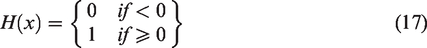
We invoke the growth trend g(t) as a core component of the entire Prophet model. The trend illustrates how the entire time series expands and how it is projected to evolve in the future. For analysts, Prophet proposes two models: a piecewise-linear model and a saturating-growth model.

Nonlinear, saturating growth is modeled using the logistic growth model, which occurs as follows in its most basic form:

g (t) = \frac{C}{1 + e x p^{- k (1 - m)}}

(4)

where m is an offset parameter, k is the growth rate, and C is the carrying capacity. However, the value of C is not inherently a constant, which usually varies over time. It was then replaced by a time-varying capability C(t). Moreover, the growth rate of k is not constant. Therefore, it is presumed that the change-point where growth rates change has been integrated and the growth rate between two change-points is constant.

The piecewise logistic-growth model is formed as follows:

g (t) = \frac{C}{1 + e x p^{- (k + a {(t)}^{T} δ) (t - (m + a {(t)}^{T} γ))}}

(5)

where γ is the vector of rate adjustments, δ is the vector of correct adjustments at change-points, and

k + a {(t)}^{T} δ

is the growth rate at time t. a(t) is defined by the following:

a (t) = {\begin{matrix} 1 & t \geq s \\ 0 & otherwise \end{matrix}}

(6)

where, s is the time point of change in the growth rate.

Linear growth is modeled using a constant growth rate piecewise, and its formula is given as:

g (t) = (k + a {(t)}^{T} δ) t + (m + a {(t)}^{T} γ)

(7)

where a(t), k, δ, and γ are the same as the nonlinear trend model.

In the time series, seasonality reflects periodic changes daily, weekly monthly and yearly seasonality. To provide a versatile model of periodic effects, the Prophet forecasting model depends on a Fourier series. Its smooth fitting formula is given as:

s (t) = \sum_{n = 1}^{N} (a_{n} c o s (\frac{2 π n t}{P}) + b_{n} s i n (\frac{2 π n t}{P}))

(8)

where P is a regular period that the time series may have (for example, P = 7 for weekly data or P = 365 for annual data) and N is the number of such cycles that we want to use in the model. The final seasonal model appears as follows when combining all seasonal time series models in s(t) into a vector X(t):

s (t) = X (t) β

(9)

where

β Normal (0, σ^{2})

is needed before the seasonality to enforce a smoothing.

Holidays and events: To completely understand the effect on holidays of a business time series or other major events such as workover, production shutdown for operations (for example, a workover), these constraints are explicitly set by the Prophet forecast model.

Recurrent neural network (RNN)

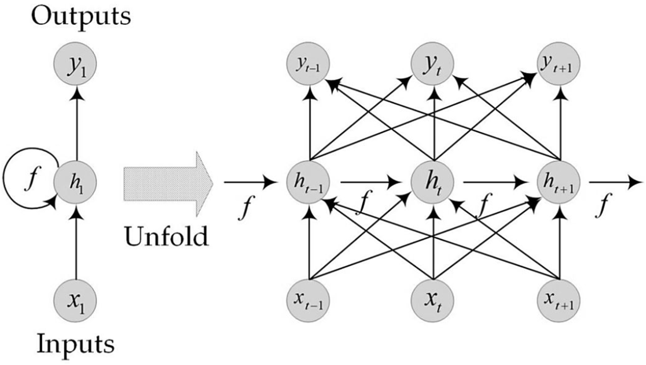
Compared with the traditional artificial neural network (ANN), the structure of RNN neuron is different from that of ANN by adding a cyclic connection, which form feedback loops in hidden layers, and hence the information of the last item in RNN can be transmitted to the current item. The structure of RNN neuron is shown in Figure 1. When the time series $X = (x_{1}, x_{2}, x_{3}, \dots, x_{n})$ is input, the sequence of hidden layer is $H = (h_{1}, h_{2}, h_{3}, \dots, h_{y})$ and the sequence of output layer is $Y = (y_{1}, y_{2}, y_{3}, \dots, y_{n})$ .

Figure 1.

The structure of Recurrent Neural Network.

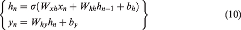
The relationship of X, H and Y are listed in the following equations:

{\begin{array}{l} h_{n} = σ (W_{x h} x_{n} + W_{h h} h_{n - 1} + b_{h}) \\ y_{n} = W_{h y} h_{n} + b_{y} \end{array}}

(10)

where, σ is the non-linear activation function, W_xh, W_hh and W_hy are the weight matrix from input to hidden layer, hidden layer to hidden layer and hidden layer to output, respectively, b_h and b_y are biased terms.

Long short-term memory neural network (LSTM)

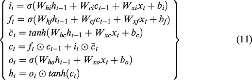
The LSTM neural network model (Greff et al., 2017; Hochreiter and Schmidhuber, 1997) is a type of RNN structure, which is widely used to solve sequence problems. An LSTM tends to learn long -term dependencies and solve the vanishing gradient problems¹ (Grosse, 2017), an issue observed in training ANN with gradient based learning techniques as well as backpropagation algorithms. An LSTM allows the storage of information extracted from data over an extended time period, and shares the same parameters (i.e., network, weights) across all timesteps.

The structure of the LSTM shown in Figure 2 consists of the long term state $(c_{t})$ and three multiplicative units N with g $(i_{t})$ , output gate $(o_{t})$ , and forget gate $(f_{t})$ — and equivalently write, read, and reset information within the model’s cells. These three multiplicative gates enable the LSTM memory cells to store and access information over long time periods. The gates control the amount of information fed into the memory cell at a given timestep. Unlike traditional RNN methods that overwrite new content at each timestep, the LSTM state vector and weights are modified at each timestep to take into account any evolution of the input-output relation occurring over time and carry that information over a long distance. The LSTM functions are listed as follows:

{\begin{array}{l} i_{t} = σ (W_{h i} h_{t - 1} + W_{c i} c_{t - 1} + W_{x i} x_{t} + b_{i}) \\ f_{t} = σ (W_{h f} h_{t - 1} + W_{c f} c_{t - 1} + W_{x f} x_{t} + b_{f}) \\ {\bar{c}}_{t} = \tanh (W_{h c} h_{t - 1} + W_{x c} x_{t} + b_{c}) \\ c_{t} = f_{t} ⊙ c_{t - 1} + i_{t} ⊙ {\bar{c}}_{t} \\ o_{t} = σ (W_{h o} h_{t - 1} + W_{x o} x_{t} + b_{o}) \\ h_{t} = o_{t} ⊙ \tanh (c_{t}) \end{array}}

(11)

where the input gate

(i_{t})

, a forget gate

(f_{t})

and previous cell state

({\bar{c}}_{t})

control the current cell state

(h_{t})

, and the output gate

(o_{t})

and current cell state

(c_{t})

are used to control the hidden state

(h_{t})

at time t. σ is the element-wise sigmoid function,

⊙

denotes the elementwise dot product operator,

(x_{t})

is the input vector at time t, and

h_{t - 1}

is the hidden state vector that store all the useful information prior to time t. W_xi, W_xf, W_xc, and W_xo denote the weight matrices of different gates for input

(x_{t})

; W_hi, W_hf, W_hc, and W_ho are the weight matrices for hidden state h_t; W_ci, and W_cf denote the weight matrices of cell state

c_{t - 1}

; and b_i, b_f, b_c, and b_o denote the bias vector.

Figure 2.

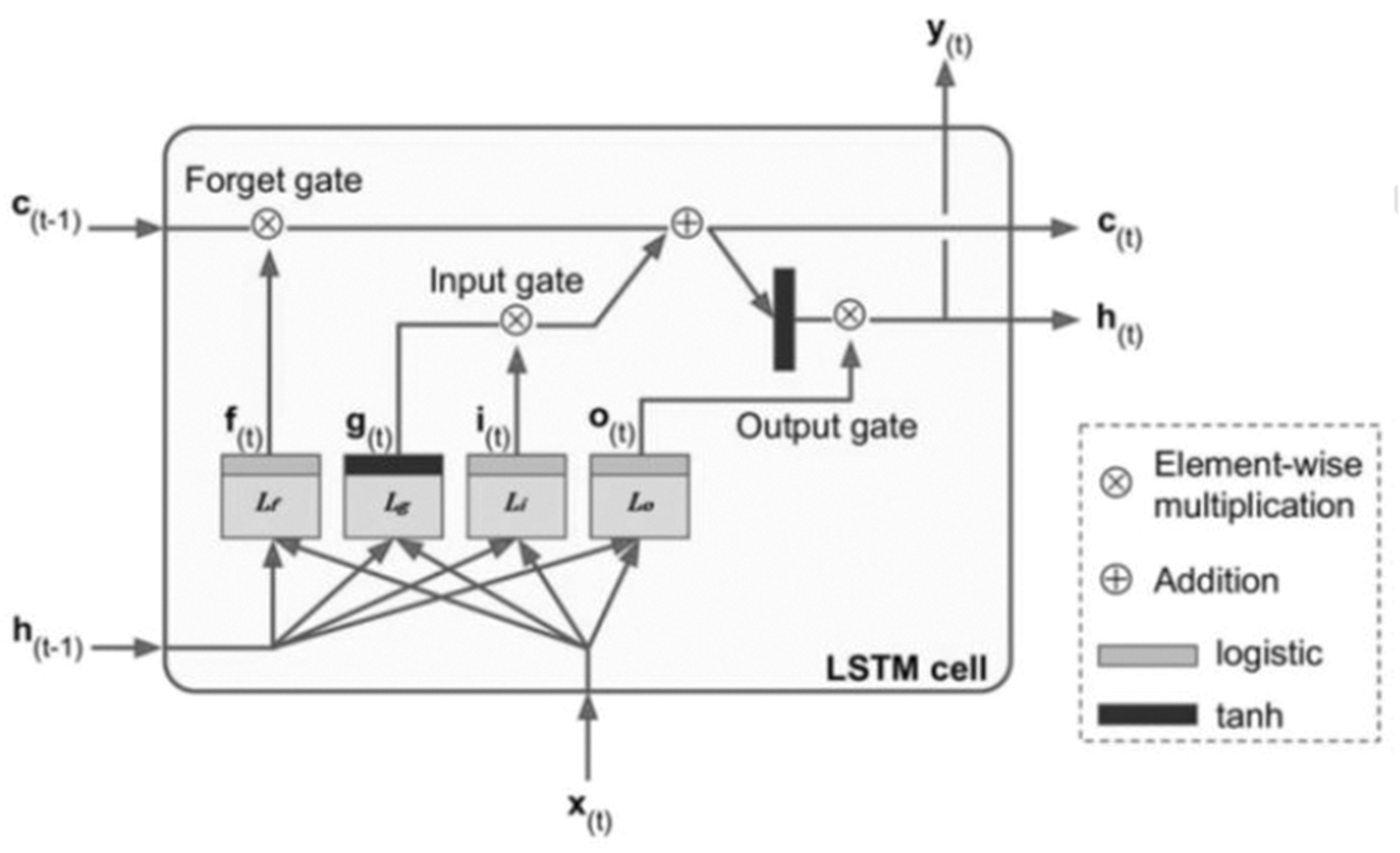
Architecture of an LSTM cell (Geron, 2017).

Gated recurrent unit (GRU)

The GRU is similar to the LSTM, but with a simplified structure and parameters. It was first introduced by (Kyunghyun et al., 2014). GRUs have been used in a variety of tasks that require capturing long-term dependencies (Junyoung et al., 2014). Similar to the LSTM, the GRU contains gating units that modulate the flow of information inside the unit. However, unlike the LSTM, the GRU does not include separate memory cells, and contains only two gates—the update gate and the reset gate—as displayed Figure 3. The update gate $z_{t}$ decides how often the unit updates its activation functions. This process takes a linear sum between the existing state and a newly computed state. The second gate within the GRU, the reset gate $r_{t}$ , acts to forget the previously computed state. The updated functions are listed as follows:

{\begin{array}{l} h_{t} = (1 - z_{t}) h_{t - 1} + z_{t} {\tilde{h}}_{t}) \\ z_{t} = σ (W_{z} x_{t} + U_{z} h_{t - 1}) \\ {\tilde{h}}_{t} = \tanh (W x_{t} + U (r_{t} ⊙ h_{t - 1})) \\ r_{t} = σ (W_{r} x_{t} + U_{r} h_{t - 1})) \end{array}}

(12)

where the activation h_t of the GRU at time t is a linear interpolation between the previous activation

h_{t - 1}

and the candidate activation

{\tilde{h}}_{t}

, W denotes the weight matrices, x_t is the input vector at time t, and U denotes the weight matrices of the cell state.

Figure 3.

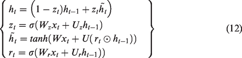
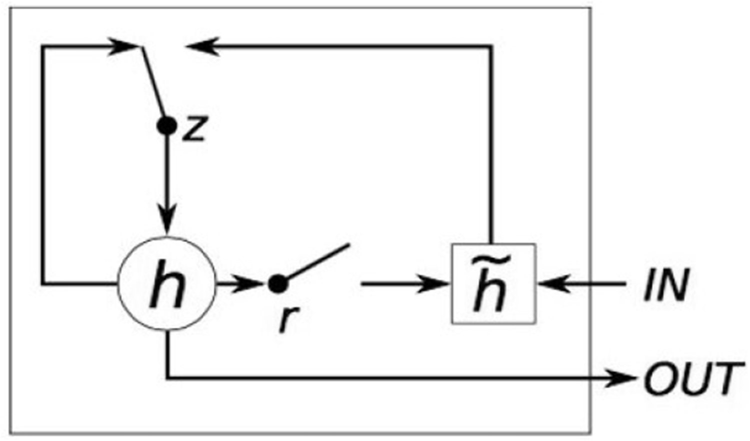
Gated Recurrent Unit: $r)$ and z are the reset and update gates, and h_t and ${\tilde{h}}_{t}$ are the activation and the candidate activation (Kyunghyun et al., 2014).

DeepAR

DeepAR is a generative, auto-regressive model. It consists of a recurrent neural network (RNN) using Long Short-Term Memory (LSTM) or Gated Recurrent Unit (GRU) cells that takes the previous time points and covariates as input. In this study, We use the forecasting model from Salinas et al. (David et al., 2019). Unlike other methods of forecasting, DeepAR jointly learns from every time series. In (David et al., 2019) publication, DeepAR was outperforming the state-of-the-art forecasting methods on many problems.

Let $z_{i, t}$ be the value of time series i at time t, the objective is to model the conditional distribution $P (z_{i}, t_{0 : T} | z_{i, 1 : t_{0} - 1}, x_{i, 1 : T})$ , of the future of each time series $[z_{i, t_{0}}, z_{i, t_{0 + 1}}, \dots, z_{i, T}] : = z_{i, t_{0 : T}}$ , given its past $[z_{i, 1}, \dots, z_{i, t_{0 - 2}}, z_{i, t_{0 - 1}}] : = z_{i, 1 : t_{0 - 1}}$ , where t₀ represents the time point from which $z_{i, t}$ is assumed to be unknown at prediction time, and $x_{i, 1 : T}$ are covariates that are presumed to be known for all time points. The time ranges $[1 : t_{0} - 1]$ and $[t_{0} : T]$ are the context range and the prediction range, respectively. The model is based on an auto-regressive recurrent network, summarised in Figure 4. The model distribution $Q_{Θ} (z_{i, t_{0}} | z_{i, 1 : t_{0}}, x_{i, 1 : T}), x_{i, 1 : T}$ is considered to be a product of likelihood factors:

\begin{array}{l} Q_{Θ} (z_{i, t_{0}} | z_{i, 1 : t_{0}}, x_{i, 1 : T}) = \prod_{t = 0}^{T} Q_{Θ} (z_{i, t} | z_{i, 1 : t - 1}, x_{i, 1 : T}) \\ = \prod_{t = 0}^{T} l (z_{i, t} | θ (h_{i, t}, Θ)) \end{array}

(13)

with

h_{i, t}

the autoregressive recurrent network output

h_{i, t} = h (h_{i, t - 1}; z_{i, t - 1}; x_{i, t}; Θ)

which will be fed as the next timestep input for

h_{i, t + 1}

h (\cdot)

is a function that is implemented by a multi-layer recurrent neural network with LSTM or GRU cells parametrized by Θ, and the likelihood

l (z_{i, t} | θ (h_{i, t}, Θ)

being a fixed distribution parametrized by a function

θ (h_{i, t}, Θ)

. The

h_{i; t_{0} - 1}

, initial state contains

z_{i; t_{0} - 1}

, context range information required to predict values in the prediction range.

Figure 4.

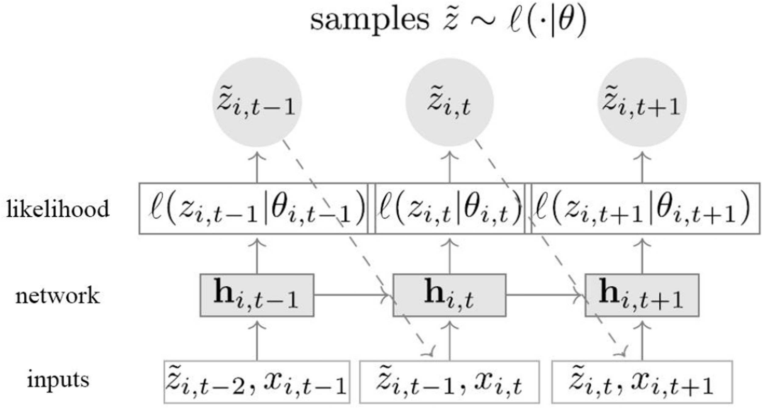
Model Summary: The network inputs are the covariates $x_{i, t}$ at each step t, the goal value at the previous step $z_{i, t - 1}$ , and the previous network output $h_{i, t - 1}$ at each step t. The network output $h_{i, t} = h (h_{i, t - 1}; z_{i, t - 1}; x_{i, t}; Θ)$ is then used to measure the parameters $θ_{i, t} = θ (h_{i, t}, Θ)$ of the probability $l (z | θ)$ that is used to train the parameters of the model. A sample ${\hat{z}}_{i, t} \sim l (\cdot | θ_{i, t})$ is fed back to the next step instead of the true value when $z_{i, t}$ is unknown (David et al., 2019).

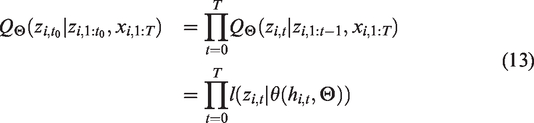
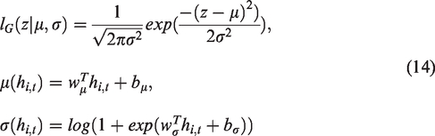
Given the model parameters required to pred ${\hat{z}}_{i, t_{0} : T} \sim Q_{Θ} (z_{i, t_{0}} | z_{i, 1 : t_{0}}, x_{i, 1 : T})$ can be obtained directly by ancestral sampling: First, $h_{i, t_{0} - 1}$ is obtained as as a recurrent network output, then we sample ${\hat{z}}_{i, t_{0} : T} \sim l (\cdot | θ ({\hat{h}}_{i, t}, Θ))$ for $t = 1, \dots, t_{0} - 1$ , where ${\hat{h}}_{i, t} = h (h_{i, t - 1}, {\hat{z}}_{i, t - 1}, x_{i, t}, Θ)$ is initialized with ${\hat{h}}_{i, t_{0} - 1} = h_{i, t_{0} - 1}$ and ${\hat{z}}_{i, t_{0} - 1} = z_{i, t_{0} - 1}$ . The use of these samples makes it possible to calculate quantities, like the value distribution quantities, at a particular time in the prediction range.

Likelihood model

The probability of $l (z | θ)$ should at best reflect the data statistical properties. It can be selected between any potential possibility, for example, Bernoulli, Gaussian, Binomial-negative, etc.

For instance, the mean and the standard deviation are the parameters $θ = (μ, σ)$ in the Gaussian likelihood case. These are provided to the network output respectively by the network output and softplus activation to ensure $σ > 0$ :

\begin{array}{l} l_{G} (z | μ, σ) = \frac{1}{\sqrt{2 π σ^{2}}} e x p (\frac{- {(z - μ)}^{2})}{2 σ^{2}}), \\ ` \\ μ (h_{i, t}) = w_{μ}^{T} h_{i, t} + b_{μ}, \\ σ (h_{i, t}) = \log (1 + \exp (w_{σ}^{T} h_{i, t} + b_{σ})) \end{array}

(14)

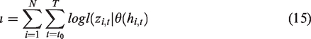
Loss function

The model parameter Θ which consists of the RNN $h (\cdot)$ parameters and the $θ (\cdot)$ parameters, can be learned by maximizing the log-likelihood, as follows:

ι = \sum_{i = 1}^{N} \sum_{t = t_{0}}^{T} l o g l (z_{i, t} | θ (h_{i, t})

(15)

with the time series dataset

z_{i, 1 : T}_{i : 1, \dots, N}

and known related covariates

x_{i; 1 : T}

. No inference is needed to calculate the previous equation compared to state-space models with latent variables, as

h_{i, t}

is a deterministic input function. It can therefore be explicitly optimized with respect to θ with stochastic gradient descent.

Measures for evaluating forecast

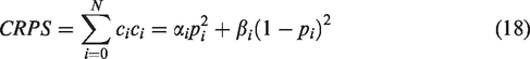
As previously mentioned, the purpose of this task is to predict several future timesteps in the target time series. Confidence intervals are also given and predicting the exact values (such as point forecasting). These are based on percentiles calculated from a probability distribution based on a fixed number of samples (e.g. DeepAR model). To evaluate the forecast accuracy, we use the mean continuous ranked probability score (mean CRPS).

Mean (CRPS): used to quantify both the accuracy and precision of a probabilistic forecast (Hersbach, 2000). A higher value of mean CRPS indicates less accurate results. CRPS can be defined as:

CRPS = \int_{- \infty}^{\infty} {[p (x) - H (x - x_{obs})]}^{2} d x

(16)

Here,

p (x) = \int_{- \infty}^{x} p (y) d_{y}

is the cumulative distribution of a quantity of interest, and

H (x - x_{obs})

is the step function, i.e.,

H (x) = {\begin{matrix} 0 & i f < 0 \\ 1 & i f ⩾ 0 \end{matrix}}

(17)

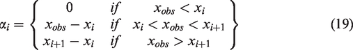
For N samples, the CRPS can be evaluated as follows:

CRPS = \sum_{i = 0}^{N} c_{i} c_{i} = α_{i} p_{i}^{2} + β_{i} {(1 - p_{i})}^{2}

(18)

where

p_{i} = P (x) = i / N, for x_{i} < x < x_{i + 1}

(piecewise constant function).

α_{i} = {\begin{matrix} 0 & i f & x_{obs} < x_{i} \\ x_{obs} - x_{i} & i f & x_{i} < x_{obs} < x_{i + 1} \\ x_{i + 1} - x_{i} & i f & x_{obs} > x_{i + 1} \end{matrix}}

(19)

β_{i} = {\begin{matrix} x_{i + 1} - x_{i} & i f & x_{obs} < x_{i} \\ x_{i + 1} - x_{obs} & i f & x_{i} < x_{obs} < x_{i + 1} \\ 0 & i f & x_{obs} > x_{i + 1} \end{matrix}}

(20)

Data collection and preparation procedure

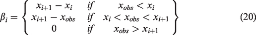
In this work, we use oil production data from wells in the Midland field. We have selected 22 Midland wells, relatively smooth data, which indicates fewer significant operational changes. The selected Midland wells have been completed in a natural fractured reservoir and measured monthly. However, there are some missing measurements (i.e., no recorded values) for a few months for each selected well. We simply ignore these missing values. Some measurements have recorded zero values, and we suspect they indicate temporary shut-down for operations (e.g., a workover). The zero values may interfere with the training process, so we remove them from the data, then the datasets are rescaled with a standardization.The standardization is included in deep learning to improve neural networks convergence. Table 1 lists the lengths of production history of the selected wells. The lengths range from 105 to 362 months. No matter how long a well’s production history is, we use the data of the last 24 months (regarded as a short term) for the blind test. Taking Well-ID3 as an example: As shown in Figure 5, the data covers 108 months. The data from Month 1 to 84 are used for building training and forecasting model using DeepAR and Prophet model, and the data from Month 85 to 108 are used for blind testing to assess the performance of prediction results. The same procedure is applied to the 22 selected wells individually.

Table 1.

Production history length of selected midland field wells.

Well-ID	3	5	8	9	11	14	15	16	17	18	20
Length (months)	108	105	105	109	106	308	315	319	362	344	311
Well-ID	21	22	72	142	156	157	171	181	206	249	524
Length (months)	314	307	112	235	246	253	162	136	134	133	105

Table 2.

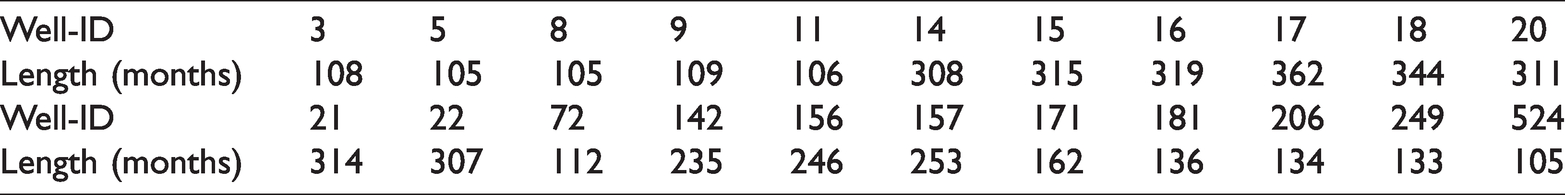
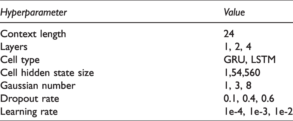
DeepAR fixed training hyperparameters.

Hyperparameter	Value
Epochs	100
Batch size	32
Batches/epoch	100

Table 3.

DeepAR hyperparameters to optimize for each well.

Hyperparameter	Value
Context length	24
Layers	1, 2, 4
Cell type	GRU, LSTM
Cell hidden state size	1,54,560
Gaussian number	1, 3, 8
Dropout rate	0.1, 0.4, 0.6
Learning rate	1e-4, 1e-3, 1e-2

Figure 5.

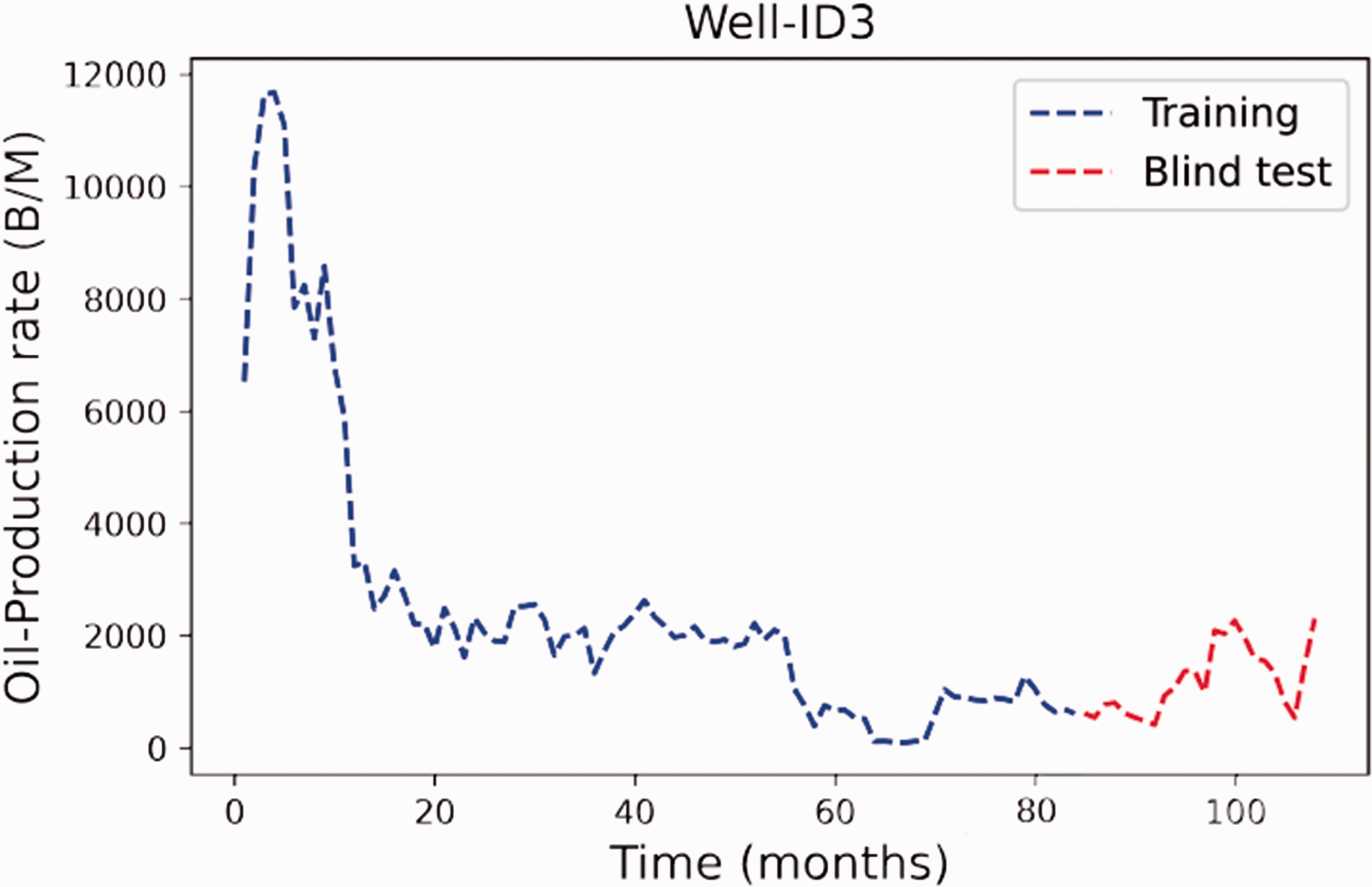
History of oil production rate, Well-ID3.

Models implementation

The two models considered, DeepAR and the Prophet time series, are evaluated based on Midland datasets. The experimental setup which is shared for each dataset evaluation is first described before the dataset experiments.

DeepAR

DeepAR is a model presented by (David et al., 2019) and then implemented in Gluon Time Series (GluonTS). GluonTS is a toolkit developed by Amazon scientists based on the Gluon framework (Alexander et al., 2019). It aims to regroup all the tools required to build deep learning models for time series forecasting and anomaly detection. DeepAR configurations are trained as it is not implemented without early stopping during its optimization (cf. Tables 2 and 3). If necessary, the final models are trained on the best parameters without early stopping or validation failure on a new training set. For each selected wells, the optimization is performed on the following parameters:

The context length and the learning rate: The number of prior timesteps taken to make the most precise forecasts. The tested context lengths depend on the data provided.

Stacking layer number: The number of layers in the recurrent neural network.

The cell type: Cell type in the recurrent neural network (GRU or LSTM).

The number of gaussians: The number of Gaussians considered to be the probability distribution of each timestep in Gaussians' mixture.

The dropout rate: The output of each LSTM cell is feed to a Zoneout² cell which uses this dropout rate (David et al., 2017).

Prophet time series implementation

An open-source implementation of the Temporal Prophet time series model that was published with the paper (Taylor and Letham, 2007) can be found on this web documentation. For each well, the main hyperparameters which can be tuned are:

Changepoint prior scale: This is likely the parameter that is most impactful. It determines the trend change points in particular. If it is, too, the trend will overfit,if it is too small, the trend will be underfitting, and variation that should have been modeled with trend changes will be treated with the noise term instead. The default value of 0.05 works for several time series, but this can be tuned; the range is [0.001, 0.5].

Sasonality prior scale: This parameter regulates the flexibility of seasonality. Similarly, a large value helps the seasonality respond to large variations, a small value shrinks the magnitude of the seasonality. The default parameter is 10, with practically no regularisation being applied. This is because overfitting occurs here very rarely (there is inherent regularisation because it is modeled with a truncated Fourier sequence, so it is filtered practically low-pass). [0.01, 10] would possibly be a good range for tuning it.

Growth: Options are ‘linear’ and ‘logistic’.

Results

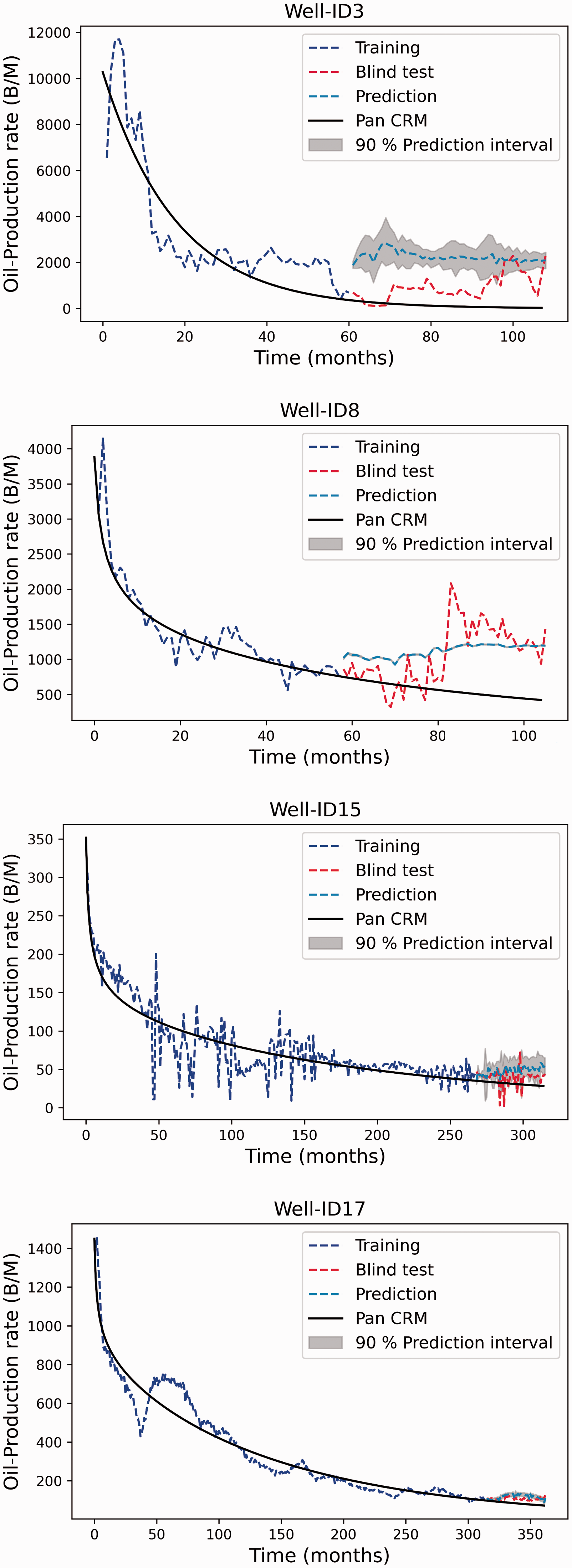
Figure 6 demonstrates the forecast results for some selected wells using the DeepAR, the means of forecasts (dashed steel blue curve) comparing to blind-test data (dashed red curve) and Pan CRM model (black line curve). In general, the production forecast seems to be reasonable, the DeepAR model can forecast both the upward and downward trends generally well and outperform the Pan CRM model, it is observed that the prediction intervals are, mostly, containing the correct values, except for the well-ID11, this could be explained by being incapable of predicting when changes in production are going to happen. We quantify the accuracy of the probabilistic forecast using the mean CRPS score as listed in Table 4. The results for prediction accuracy are quite satisfactory. In most cases, the mean CRPS decreases as the length of production history increases. This indicates that a longer production history (i.e., more data) will improve the DeepAR model forecast. A major drawback of DeepAR is that it has very little to no interpretability. We cannot interpret any physical meanings from the trained DeepAR model parameters.

Figure 6.

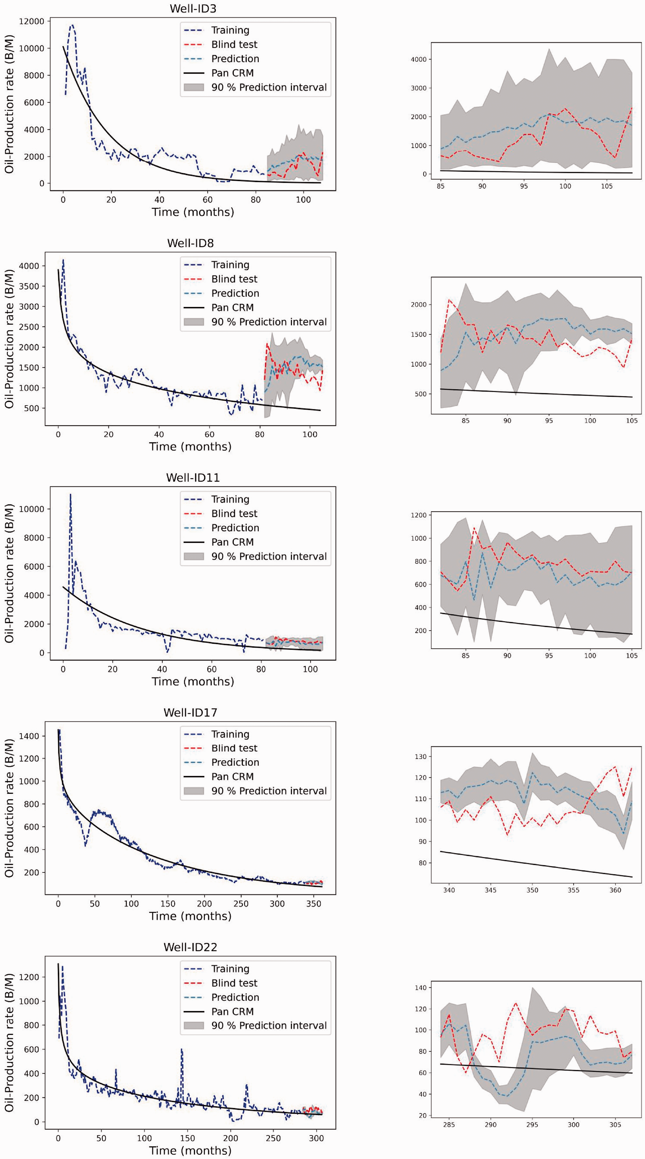
Oil production time series forecast - DeepAR. Left: Overview of forecast. Right: zoomed forecast.

Table 4.

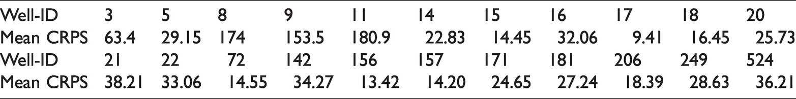
Mean CRPS of probabilistic forecast from DeepAR model.

Well-ID	3	5	8	9	11	14	15	16	17	18	20
Mean CRPS	69	29.15	74	93.5	80.9	15.25	7.89	19.17	9.91	12.01	15.18
Well-ID	21	22	72	142	156	157	171	181	206	249	524
Mean CRPS	23.18	22.14	8.35	27.39	3.47	10.50	21.67	21.37	19.69	27.80	29.91

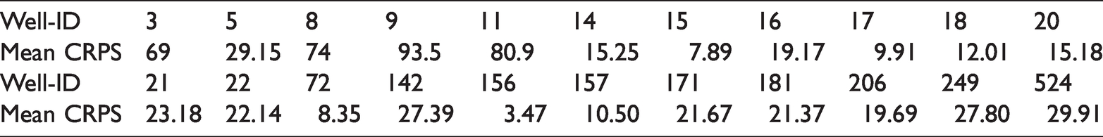
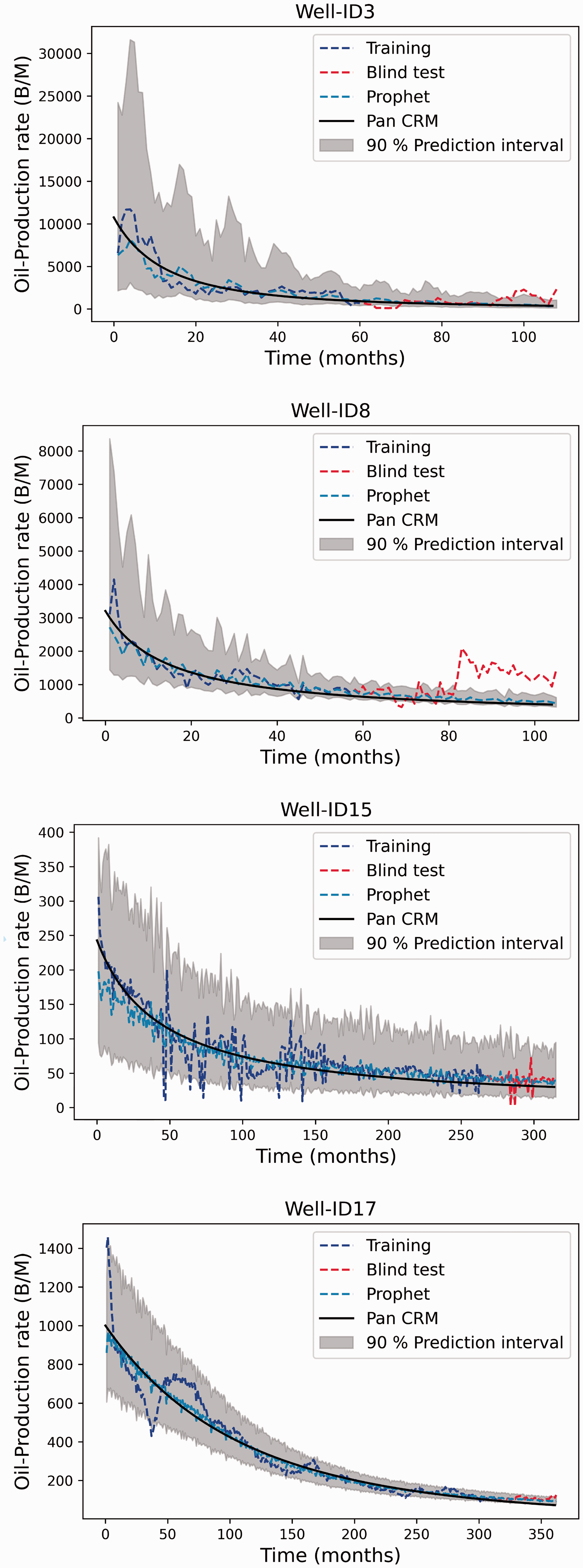
Figure 7 shows forecasts from the trained Prophet models. The means of forecasts (the dashed Steel blue curve) follow the blind-test data (dashed red curve in Figure 7) generally well. The P5-P95 prediction intervals (grey band in Figure 7) covers most of the blind-test data. However, for Well-ID8, the forecast significantly deviates from blind-test data and fails to capture both trends and the peaks and troughs reasonably; more specifically, the forecast underestimates the oil production rates.

Figure 7.

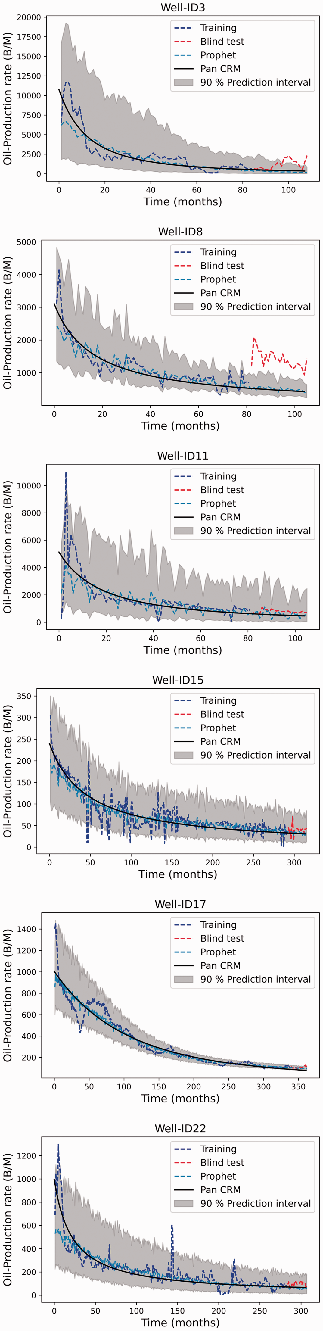
Oil production time series forecast - Prophet.

Compared to Prophet, the DeepAR models represent distinct trends in the mean CRPS score as listed in Table 5. This is possibly due to the DeepAR layer’s capacity to “memorize” long-term patterns. In contrast, Prophet’s predictions rely majorly on the pattern of the most previous historical data. Besides, DeepAR indicates that the lowest CRPS errors arise. Simultaneously, the difference in values is minimal, even though this statement is only valid for the 5-th and 95-th percentileses. This is demonstrated by the better coverage earned by the longer periods that compensate for the 50-th percentile's low accuracy.

Table 5.

Mean CRPS of probabilistic forecast from Prophet model for each well.

Well-ID	3	5	8	9	11	14	15	16	17	18	20
Mean CRPS	63.4	29.15	174	153.5	180.9	22.83	14.45	32.06	9.41	16.45	25.73
Well-ID	21	22	72	142	156	157	171	181	206	249	524
Mean CRPS	38.21	33.06	14.55	34.27	13.42	14.20	24.65	27.24	18.39	28.63	36.21

Limitation: In the previous section, we presented DeepAR and Prophet trends in the mean CRPS score as liste months (2 years). We evaluate the performance of the two methods for a forecast horizon of 48 months, as displayed in both Figures 8 and 9, It can be obviously seen that the two methods exhibited quite similar performance almost equally well when the length of wells more than 300 months, for the most part, they well capture the trends of oil production rate in blind tests, and the predictions yielded by each of the models appear to be quite similar. The models were good at predicting trends and flat lines, but sometimes undershot/overshot the peaks and troughs, i.e., Well-ID8. However, both the Prophet and DeepAR did not match production data including quantifying uncertainty, with a small historical data length. Based on the previous results, we can highlight that the two methods enrich the family of time series analysis models by extracting the weighted differencing/trend feature, and contribute to better performance in short-term oil production forecasts, and it can be an alternative way for oil production forecasting in practical application.

Figure 8.

Oil production time series forecast- DeepAR - 48 months horizon forecast.

Figure 9.

Oil production time series forecast- Prophet - 48 months horizon forecast.

Discussion and conclusion

The purpose of this work is to demonstrate a method of machine learning that could replace or accelerate manual DCA for short-term oil and gas well forecasting. Probabilistic Prophet time series analysis and more accurate deep learning models, DeepAR, were considered to solve this problem. These two have been selected as they outperform the state-of-the-art methods of forecasting on many topics. For time series forecasting, Prophet is a Bayesian non-linear univariate generative model proposed by Facebook. The Prophet is also a structural time series analysis method that specifically models the impact of patterns, seasonality, and events. For the Prophet, the cyclical duration and event date parameters are set the same as our model. In contrast, DeepAR is an auto-regressive model based on cells with GRU or LSTM recurrent neural networks. It learns the parameters for each forecast horizon from a given probability allocation. Then, by sampling several times, one can sample from certain probability distributions to forecast each horizon or compute confidence intervals. The model validation was carried out on 22 separate midland reservoir field oil production datasets. Each has had their outliers removed and missing data replaced. They were also standardized as a pre- and post-processing to increase the model’s accuracy. Their performances were evaluated based on mean CRPS metrics. The prediction length was initially fixed to 24 months and planned to be increased to 48 months. The models first went through a hyperparameter optimization to select to optimal parameters of each methods of each well. The results showed that the deep learning approach and Prophet analysis yield a satisfactory result in short term forecast, but they may fail to identify long-term trends in predictions unless the predictions are constantly adjusted. However, The both approaches relies on the volume and granularity of data to develop capability for predicting production over a long-time horizon.

This approach can be regarded as “model-free” because, unlike the traditional DCA, the selection of a specific decline curve model is not required. However, It is important to highlight some potential drawbacks of applying time series deep learning for oil production prediction. Deep learning models may suffer significant errors when used for long-term forecasts. This is in addition to their limited interpretability. That is because the predictions are computed sequentially and depend on past predictions that have been appended to the data. Thus, there is a gradual accumulation of error over time. Deep learning models have to be retrained periodically as more data are collected. Otherwise, their predictions become highly inaccurate after a long period. Furthermore, another difficulty that may arise when applying deep learning is that an intermediate-to-expert level of knowledge may be required during model creation and training, as opposed to other out-of-the-box machine learning methods that can be trained easily by adjusting their hyperparameters. Therefore, general NNs may require some adjustments to their cell architecture.

In conclusion, the precise prediction and learning performance presented in the paper suggests that both Prophet and DeepAR are eligible for use in the petroleum industry’s non-linear short-term forecasting problems. Many steps should be taken to further improve the performance of forecasting over long time horizons, such as the application to spatiotemporal tasks or the use of an encoder-decoder from sequence to sequence, where the contextual data (static and dynamic) would be integrated into the model architecture. Additionally, integrating physics constraints during the training of a deep neural network. An advantage of such approach is that physics can be introduced into ML approaches and could replace or speed up manual DCA to perform long term forecast of oil and gas well.

Footnotes

Acknowledgements

The authors acknowledge financial support from the Research Council of Norway through the Petromaks-2 project DIGIRES (RCN no. 280473) and the industrial partners AkerBP, Wintershall DEA, Vår Energi, Petrobras, Equinor, Lundin, and Neptune Energy.

Declaration of conflicting interests

The author(s) declared no potential conflicts of interest with respect to the research, authorship, and/or publication of this article.

Funding

The author(s) received no financial support for the research, authorship, and/or publication of this article.

Notes

References

Adekoya

(2009) Production decline analysis of horizontal well in gas shale reservoirs. Master thesis, West Virginia University, Morgantown, WV, USA.

Aditya

Akhil

Srikanta

(2017) Modeling early time rate decline in unconventional reservoirs using machine learning techniques. In: Abu Dhabi international petroleum exhibition & conference, Abu Dhabi, UAE, 13–16 November.

Alexander

Konstantinos

Michael

, et al. (2019) Gluonts: Probabilistic time series models in python. Available at: https://arxiv.org abs/1906.05264

Arps

(1945) Analysis of decline curves. Trans.

Cho

van Merrienboer

Bahdanau

, et al. (2014) On the properties of neural machine translation: Encoder-decoder approaches. In: Eighth workshop on syntax, semantics and structure in statistical translation. Available at: https://nyuscholars.nyu.edu/en/publications/on-the-properties-of-neural-machine-translation-encoder-decoder-a

David

Tegan

János

, et al. (2017) Zoneout: Regularizing rnns by randomly preserving hidden activations.

David

Valentin

Jan

(2019) Deepar: Probabilistic forecasting with autoregressive recurrent networks.

Duong

(2011) Rate-decline analysis for fracture-dominated shale reservoir. SPE Reservoir Evaluation & Engineering 14(3): 377–387.

Gasthaus

Benidis

Wang

, et al. (2019) Probabilistic forecasting with spline quantile function rnns. In: Proceedings of machine learning research (eds K Chaudhuri and M Sugiyama), volume 89, pp.1901–1910.

10.

George

EPB

Gwilym

Gregory

, et al. (2015) Time Series Analysis: Forecasting and Control. Hoboken: John Wiley & Sons.

11.

Geron

(2017) Hands-On Machine Learning with Scikit-Learn and TensorFlow: Concepts, Tools, and Techniques to Build Intelligent Systems. USA: OSA: Intelligent Sy

12.

Gonzalez

Gong

McVay

(2012) Probabilistic decline curve analysis reliably quantifies uncertainty in shale gas reserves regardless of stage of depletion. In: SPE eastern regional meeting.

13.

Greff

Srivastava

Koutnik

, et al. (2017) Lstm: A search space odyssey. IEEE Transactions on Neural Networks and Learning Systems 28(10): 2222–2232.

14.

Grosse

(2017) Lecture 15: Exploding and vanishing gradient. Available at: www.cs.toronto.edu/∼rgrosse/courses/csc321_2017/readings/L15\%20Exploding\%20and\%20Vanishing\%20Gradients.pdf

15.

Gupta

Fuehrer

Benin

(2014) Production forecasting in unconventional resources using data mining and time serie analysis. In: SPE/CSUR unconventional resources conference, Canada, 30 September–2 October 2014.

16.

Han

Jung

Kwon

(2020) Comparative study on supervised learning models for productivity forecasting of shale reservoirs based on a data-driven approach. Applied Sciences 10(4): 1267.

17.

Hersbach

(2000) Decomposition of the continuous ranked probability score for ensemble prediction systems. weather and forecasting. Weather and Forecasting 15(5): 559–570.

18.

Hochreiter

Schmidhuber

(1997) Long short term memory. Neural Computation 9(8): 1735–1780.

19.

Hong

Bratvold

Lake

, et al. (2019) Integrating model uncertainty in probabilistic decline-curve analysis for unconventional-oil-production forecasting. SPE Reservoir Evaluation & Engineering 22(3): 861–876.

20.

Joshi

(2012) Comparison of various deterministic forecasting techniques in shale gas reservoirs with emphasis on the duong method. PhD thesis, Texas A&M University, College Station, TX, USA.

21.

Junyoung

Caglar

KyungHyun

, et al. (2014), Empirical evaluation of gated recurrent neural networks on sequence modeling.

22.

Kyunghyun

Bart van

Caglar

, et al. (2014) Learning phrase representations using rnn encoder-decoder for statistical machine translation.

23.

Lee

Lim

Yoon

, et al. (2019) Prediction of shale-gas production at duvernay formation using deep-learning algorithm. SPE Journal 24(6): 2423–2437.

24.

Liu

(2020) Forecasting oil production using ensemble empirical model decomposition based long short-term memory neural network. Journal of Petroleum Science and Engineering 189: 107013.

25.

Luo

Tian

Sharma

, et al. (2019) Eagle ford well insights using data-driven approaches. In: International petroleum technology conference, Beijing, China, March 2019.

26.

Liu

(2018) Predicting the oil production using the novel multivariate nonlinear model based on arps decline model and kernel method. Neural Computing and Applications 29(2): 579–591.

27.

Nelson

(2009) Pore-throat sizes in sandstones, tight sandstones, and shales. AAPG Bulletin 93(3): 329–340.

28.

Jordan

(2002) On discriminative vs. generative classifiers: A comparison of logistic regression and naive bayes. Advances in Neural Information Processing Systems 14: 841–848.

29.

Pan

(2016) Revised productivity index equation to improve transient history match for the capacitance resistance model. Master thesis, University of Texas at Austin, Austin, USA.

30.

Ruofeng

Kari

Balakrishnan

, et al. (2018), A multi-horizon quantile recurrent forecaster.

31.

Sagheer

Kotb

(2019) Time series forecasting of petroleum production using deep lstm recurrent networks. Neurocomputing 323: 203–213.

32.

Taylor

Letham

(2007) Forecasting at scale.

33.

Valkó

Lee

(2010) A better way to forecast production from unconventional gas wells. In: SPE annual technical conference and exhibition.

34.

Wattenbarger

El-Banbi

Villegas

, et al. (1998), Production analysis of linear flow into fractured tight gas wells. In: SPE Rocky Mountain Regional/low-permeability reservoirs symposium, Denver, USA, 5–8 April.

35.

Zhan

Sankaran

LeMoine

, et al. (2019) Application of machine learning for production forecasting for unconventional resources. In: Unconventional resources technology conference (URTEC).

Machine learning based decline curve analysis for short-term oil production forecast

Abstract

Keywords

Introduction

Time series analysis and DCA

Time series analysis

DCA

Machine-learning models and techniques for time series analysis

Prophet forecasting model

Recurrent neural network (RNN)

Long short-term memory neural network (LSTM)

Gated recurrent unit (GRU)

DeepAR

Likelihood model

Loss function

Measures for evaluating forecast

Data collection and preparation procedure

Models implementation

DeepAR

Prophet time series implementation

Results

Discussion and conclusion

Footnotes

Acknowledgements

Declaration of conflicting interests

Funding

Notes

References