Sage Journals: Discover world-class research

Abstract

Through the accurate prediction of power load, the start and stop of generating units in the power grid can be arranged economically and reasonably. The safety and stability of power grid operation can be maintained. First, chicken swarm optimizer based on nonlinear dynamic convergence factor (NCSO) optimizer is proposed based on chicken swarm optimizer (CSO) optimizer. In NCSO optimizer, nonlinear dynamic inertia weight and levy mutation strategy are introduced. Compared with CSO optimizer, the convergence speed and effect of NCSO optimizer are obviously improved. Second, the random parameters of extreme learning machine (ELM) model are optimized by NCSO optimizer, and NCSOELM model is established to predict the power load. Finally, the NCSO optimization extreme learning machine (NCSOELM) model is used to predict the power load, and compared with back propagation (BP), support vector machine (SVM) and CSO optimization extreme learning machine (CSOELM) model. The experimental results show that the fitting accuracy of NCSOELM model is high, and the determination coefficient r² is above 90%. And the root mean square error value of the NCSOELM model is 0.87, 0.41, and 0.25 smaller than the root mean square error values of the support vector machine, BP, and CSOELM models, respectively. Experiments show that the model proposed in this study has high fitting effect and low prediction error, which is of positive significance for the realization of economic and safe operation of energy system.

Keywords

Energy system power load forecasting extreme learning machine optimizer levy mutation strategy

Introduction

With the rapid development of social economy, people’s demand for electricity is also increasing (Abdel-Aal, 2004; Almuhtady et al., 2019; Li et al., 2017a, 2018b; Pai and Hong, 2005). Power load forecasting is based on the operating characteristics of the energy system, capacity expansion decisions, and other factors, and on the premise that certain forecast accuracy is met, load data for the future moment are determined (Caro et al., 2020; Che et al., 2012; Li et al., 2019b). The timeliness and accuracy of load forecasting have a great impact on the economic operation of energy systems (AlRashidi and El-Naggar, 2010; Chiu et al., 1997; Essallah and Khedher, 2019). Power load forecasting is an important basis for achieving economic dispatch of energy systems. Relevant research shows that the accuracy of power load forecasting has an important impact on the operating cost of energy systems, so how to improve the accuracy of power load forecasting has been a hot issue for experts (Bianco et al., 2009; Li et al., 2017b; Sharma and Ghosh, 2019).

At present, there are two kinds of power load forecasting models, one is based on time series analysis and the other is based on machine learning model (Amjady and Keynia, 2009; Chen et al., 2004; Mirasgedis et al., 2006). Time series model is based on time series. The basic idea of time series prediction model is to build a mathematical model which can reflect the dynamic dependency relationship in the series according to the limited length data (Hyndman and Khandakar, 2008; Kayacan et al., 2010). The time series analysis method is simple, easy to implement, but the accuracy of the method is poor. It is generally only suitable for a small amount of data prediction. Common time series analysis prediction methods include autoregressive moving average model, moving average model, autoregressive model, and differential autoregressive moving average model (Bennett et al., 2014; Erdogdu, 2007; Espinoza et al., 2005). Compared with time series analysis prediction model, machine learning model has stronger nonlinear prediction effect. Generally, the sample set is determined first and divided into training samples and testing samples. First, the model is trained by the training samples and then the model is tested by the testing samples. Common machine learning models include Gaussian process regression (GPR), support vector machine (SVM), neural network (NN), Bayesian model, and so on (Buitrago and Asfour, 2017; Cecati et al., 2015; Ko and Lee, 2013). NN model is suitable for large sample prediction; SVM model is suitable for small sample prediction; Bayesian model is based on conditional probability, its calculation speed is slow; GPR model has the advantages of super parameter adaptive acquisition, but its calculation cost is large.

Compared with time series prediction model, machine learning model is the focus of current research. Tang et al. (2019) established a multi-layer bi-directional recurrent NN model to predict power load, used two groups of experimental data to verify the proposed model, and considered the difference of seasonal load. Because of the non-stationary and nonlinear characteristics of load series, it will increase the difficulty of forecasting. For this reason, Mohan et al. (2018) proposed a load data-driven forecasting model based on dynamic model decomposition. The biggest advantage of this model is that it can identify the external factors that affect the characteristics of load data. Liu et al. (2019) proposed a hybrid method for power load forecasting. Due to the high noise in the original power load data, the high noise signal will affect the prediction results, so the original power load data are preprocessed to reduce the impact of noise. Then, the super parameters of SVM are optimized by whale optimizer, and finally the power load is predicted by SVM model. Ceperic et al. (2013) established the support vector regression model to predict the power load. This model uses feature selection algorithm to determine the input of the model, and uses particle swarm optimization algorithm to optimize the super parameters, so as to reduce the interaction. Cevik and Cunkas (2015) used fuzzy logic to forecast power load. In order to improve the prediction effect, first, the samples are grouped according to the load characteristics, and then the fuzzy logic is used to predict the load. For machine learning model based on kernel function, such as SVR, the choice of kernel function has great impact on the forecasting results. Che and Wang (2014) proposed a new selection algorithm to select the kernel function of the model, so as to improve the forecasting effects.

In this paper, extreme learning machine (ELM) model is used as the power load forecasting model. Compared with classical forecasting methods, ELM model has faster computing speed and stronger generalization ability. Compared with the SVM model suitable for small samples, the ELM model is less sensitive to the number of samples and is more applicable. So ELM model is used to predict the power load. First, based on CSO optimizer, NCSO optimizer is proposed. In NCSO optimizer, nonlinear dynamic convergence factor and levy mutation strategy are introduced to improve the convergence ability of the optimizer. Second, in order to improve the forecasting effects of ELM model, the parameters are optimized by NCSO optimizer, and then NCSOELM prediction model is established. Finally, the power load is forecasted by NCSOELM model and compared with SVM, BP, and CSOELM model. The test results show that the model proposed in this study has high forecasting accuracy and fitting effect. This paper has three main contributions. First, this paper proposes the NCSOELM model for power load forecasting. Second, this study proposes an NCSO optimizer and applies it to the field of load forecasting. Third, through the accurate prediction of the power load, the safe and stable operation of the power system can be guaranteed.

The rest of this paper is organized as follows. The next section introduces the basic principles of ELM model, NCSO optimizer, and NCSOELM prediction model. The “NCSO optimizer test and power load forecasting” section introduces the test process of NCSO optimizer and the prediction results of each model for power load.

Power load forecasting model

ELM model principle

The ELM is developed based on single-layer feedforward NN. Feedforward NN is more sensitive to learning rate (Liu et al., 2020a). When the learning rate is small, the convergence speed of the NN is slower and it takes longer to calculate; when the learning rate is large, the convergence of the NN is unstable (Huang et al., 2011., 2012). ELM is an improvement of feedforward NN. The learning speed and generalization ability of ELM are faster than feedforward NN. Therefore, ELM is widely used in the fields of prediction, pattern recognition, and fault diagnosis.

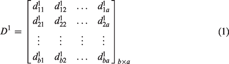
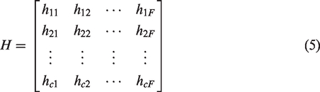
The ELM model consists of three layers: the input layer, the hidden layer, and the output layer. Each layer is composed of neural nodes, which are connected by connection weight. Suppose the input layer, the hidden layer, and the output layer have a, b, and c neural nodes, respectively. The connection weight D¹ between the input layer and the hidden layer is as follows (Huang et al., 2010; Li et al., 2015; Wang, 2016; Wang et al., 2017; Zong et al., 2013)

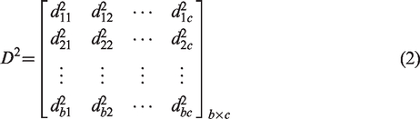
D^{1} = {[\begin{matrix} d_{11}^{1} & d_{12}^{1} & \dots & d_{1 a}^{1} \\ d_{21}^{1} & d_{22}^{1} & \dots & d_{2 a}^{1} \\ ⋮ & ⋮ & ⋮ & ⋮ \\ d_{b 1}^{1} & d_{b 2}^{1} & \dots & d_{b a}^{1} \end{matrix}]}_{b \times a}^{}

(1)

The connection weight $D^{2}$ between the output layer and the hidden layer is as follows

D^{2} = {[\begin{matrix} d_{11}^{2} & d_{12}^{2} & \dots & d_{1 c}^{2} \\ d_{21}^{2} & d_{22}^{2} & \dots & d_{2 c}^{2} \\ ⋮ & ⋮ & ⋮ & ⋮ \\ d_{b 1}^{2} & d_{b 2}^{2} & \dots & d_{b c}^{2} \end{matrix}]}_{b \times c}

(2)

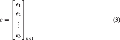
The neural node threshold of the hidden layer is as follows

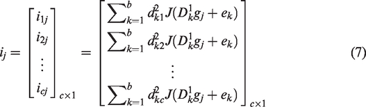
e = {[\begin{matrix} e_{1} \\ e_{2} \\ ⋮ \\ e_{b} \end{matrix}]}_{b \times 1}

(3)

Suppose that the elm model has $F$ training samples. The input matrix of the sample set is $G$ and the output matrix is $H$

G = [\begin{matrix} g_{11} & g_{12} & \dots & g_{1 F} \\ g_{21} & g_{22} & \dots & g_{2 F} \\ ⋮ & ⋮ & ⋮ & ⋮ \\ g_{a 1} & g_{a 2} & \dots & g_{a F} \end{matrix}]

(4)

H = [\begin{matrix} h_{11} & h_{12} & \dots & h_{1 F} \\ h_{21} & h_{22} & \dots & h_{2 F} \\ ⋮ & ⋮ & ⋮ & ⋮ \\ h_{c 1} & h_{c 2} & \dots & h_{c F} \end{matrix}]

(5)

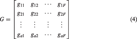
Let the activation function of the hidden layer network be $J (a)$ , then the output of the network is I

I = [\begin{matrix} i_{1} & i_{2} & \dots & i_{F} \end{matrix}]

(6)

i_{j} = {[\begin{matrix} i_{1 j} \\ i_{2 j} \\ ⋮ \\ i_{c j} \end{matrix}]}_{c \times 1} = {[\begin{matrix} \sum_{k = 1}^{b} d_{k 1}^{2} J (D_{k}^{1} g_{j} + e_{k}) \\ \sum_{k = 1}^{b} d_{k 2}^{2} J (D_{k}^{1} g_{j} + e_{k}) \\ ⋮ \\ \sum_{k = 1}^{b} d_{k c}^{2} J (D_{k}^{1} g_{j} + e_{k}) \end{matrix}]}_{c \times 1}

(7)

where

g_{j} = {[\begin{matrix} g_{1 j} & g_{2 j} & \dots & g_{a j} \end{matrix}]}^{T}

D_{k}^{1} = [\begin{matrix} d_{k 1}^{1} & d_{k 2}^{1} & \dots & d_{k a}^{1} \end{matrix}]

. Transform equation (7) as follows

L D^{2} = I^{T}

(8)

\begin{array}{l} L (D_{1}^{1}, D_{2}^{1}, \dots, D_{c}^{1}, d_{1}^{2}, d_{2}^{2}, \dots, d_{c}^{2}, g_{1}, g_{2}, \dots {,g}_{F}) \\ = [\begin{matrix} J (D_{1}^{1} \cdot g_{1} + e_{1}) & J (D_{2}^{1} \cdot g_{1} + e_{2}) & \dots & J (D_{c}^{1} \cdot g_{1} + e_{c}) \\ J (D_{1}^{1} \cdot g_{2} + e_{1}) & J (D_{2}^{1} \cdot g_{2} + e_{2}) & \dots & J (D_{c}^{1} \cdot g_{2} + e_{c}) \\ ⋮ & ⋮ & ⋮ & ⋮ \\ J (D_{1}^{1} \cdot g_{F} + e_{1}) & J (D_{2}^{1} \cdot g_{F} + e_{2}) & \dots & J (D_{c}^{1} \cdot g_{F} + e_{c}) \end{matrix}] \end{array}

(9)

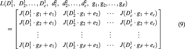
Get D² by finding the least squares solution

\min_{D^{2}} ‖ L D^{2} - I^{T} ‖

(10)

The least square solution obtained is as follows

{\hat{D}}^{2} = L^{+} I^{T}

(11)

where

L^{+}

is the generalized inverse matrix of hidden layer neural nodes.

Compared with the feedforward NN, the calculation speed of ELM model is faster. Because the connection weights and thresholds of ELMmodel are randomly initialized and remain unchanged during the model training process. However, if the random initial super parameters are not selected properly, it will increase the calculation amount and affect the forecasting accuracy of the model. Therefore, this study improves the shortcomings of ELM model and uses intelligent optimizer to optimize the super parameters.

Chicken swarm optimizer (CSO)

The chicken optimizer (CSO) imitates the hierarchy and behavior characteristics of chicken (Meng et al., 2014). The CSO optimizer includes cocks, chicks, and hens. Compared with the classical optimizer such as particle swarm optimizer and ant swarm optimizer, it has stronger convergence ability and robustness. The CSO optimizer follows these rules (Al Shayokh and Shin, 2017; Fu et al., 2019; Tiana et al., 2017):

The population is divided into groups.

In the population, the rooster is the leader; the number of hens is the most, but the foraging ability is weaker than that of the rooster; the foraging ability of the chicks is the worst and they forage around the hens.

In the CSO optimizer, the hierarchical relationship of the population is rebuilt at regular intervals.

The positions of cocks, hens, and chicks are updated according to their respective motion rules.

The location of each individual in the CSO optimizer represents a possible solution to the actual problem. There are $n$ particles in the population. Suppose the number of cocks, hens, and chicks is $n_{c}$ , $n_{h}$ , and $n_{k}$ , respectively. Assuming the flock is optimized in m-dimensional space, the position of the $i th$ chicken in the j-dimensional space at time t can be expressed as $W_{i}^{j} (t)$ .

The cock example has the best fitness value and the largest range of foraging. The cock’s position is as follows

W_{i}^{j} (t + 1) = W_{i}^{j} (t) + W_{i}^{j} (t) * Randn (0, σ^{2})

(12)

σ^{2} = {\begin{array}{l} 1 f i t_{i} \leq f i t_{k} \\ e^{\frac{f i t_{k} - f i t_{i}}{| f i t_{i} + ε |}} f i t_{i} > f i t_{k} \end{array}

(13)

where

Randn (0, σ^{2})

stands for Gaussian distribution, where 0 is the mean and

σ^{2}

is the variance.

f i t_{i}

represents the fitness value of the

i th

cock,

f i t_{k} (k \in [1, n] and k \neq i)

represents the fitness value of the other rooster, and

ε

represents the infinitesimal avoiding denominator of 0.

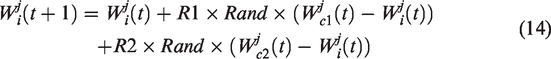
In the CSO optimizer, there is a competitive relationship between various groups, and hens can steal food from other groups. The location of the hen is as follows

\begin{array}{l} W_{i}^{j} (t + 1) = W_{i}^{j} (t) + R 1 \times Rand \times (W_{c 1}^{j} (t) - W_{i}^{j} (t)) \\ + R 2 \times Rand \times (W_{c 2}^{j} (t) - W_{i}^{j} (t)) \end{array}

(14)

R 1 = e^{\frac{f i t_{i} - f i t_{c 1}}{| f i t_{i} | + ε}}

(15)

R 2 = e^{f i t_{c 2} - f i t_{i}}

(16)

where

Rand

is the random number;

c 1 \in [1, n]

is the cock in the population of the

i th

hen;

c 1 \in [1, n] (c 1 \neq c 2)

is the cock or hen in other populations. When

R 1 = 0

, the hens scramble for food from other populations; when

R 2 = 0

, the hens only follow the males of their own populations for food.

Chicks forage around the hens, and the chicks have the smallest range of foraging. The chick’s position is as follows

W_{i}^{j} (t + 1) = W_{i}^{j} (t) + B L \times (W_{m}^{j} (t) - W_{i}^{j} (t))

(17)

where

B L \in [0, 2]

is the following coefficient;

W_{m}^{j}

is the mother chicken of the

i th

chick.

CSO based on nonlinear dynamic convergence factor (NCSO)

Nonlinear dynamic convergence factor

When the CSO optimizer is solving more complex problems, due to the limitations of the CSO optimizer itself, the optimization ability of the CSO optimizer is limited. Cock represents the strongest particle in the population, with the best fitness value and maximum search ability. If the cock, as the leader of the population, cannot jump out of the local search, the convergence ability of the whole population will be limited. Therefore, in this study, nonlinear dynamic convergence factor is introduced to improve the convergence ability of the cock.

Equation (18) shows the mathematical model of nonlinear convergence factor

Z (t) = Z_{\max} + (Z_{\max} - Z_{\min}) \times e^{{(- 10 \times (\frac{t}{t_{\max}}))}^{3}}

(18)

where

Z_{\max} = 0.9

Z_{\min} = 0.4

t_{\max}

is the maximum number of iterations, and

t

is the current number of iterations.

As shown in Figure 1, in the early stage of the iteration, the nonlinear dynamic convergence factor is large, so as to ensure that the cock has a large search range, so as to achieve a strong global optimization ability; in the middle and later stages of the iteration, the nonlinear dynamic convergence factor is small, so that the cock can achieve a strong local optimization ability.

Figure 1.

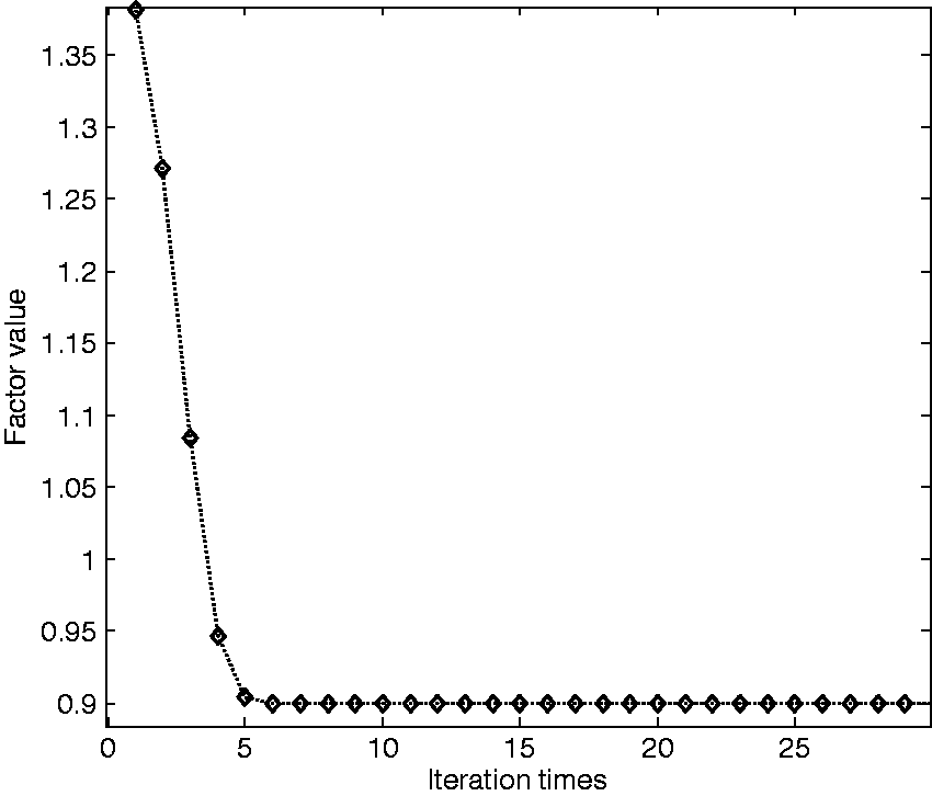
Nonlinear dynamic convergence factor.

The cock is located as follows

W_{i}^{j} (t + 1) = Z (t) \times W_{i}^{j} (t) + W_{i}^{j} (t) \times Randn (0, σ^{2})

(19)

High quality population initialization has a great impact on accelerating the convergence speed of CSO optimizer.

b. Levy mutation strategy

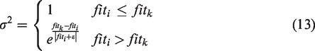
In the CSO optimizer, the fitness value of the chick is the worst and easily falls into local extremes. In this study, Levy mutation strategy was used to improve the foraging range of chicks. The foraging method based on Levy flight strategy has stronger natural adaptability. Levy distribution shows short-distance searching and occasional long-distance jumping. This method can better maintain the diversity of the population.

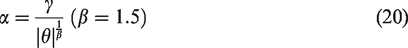
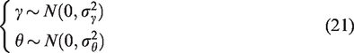
Levy’s random step size $α$ is expressed as follows

α = \frac{γ}{{| θ |}^{\frac{1}{β}}} (β =1 .5)

(20)

where

γ

and

θ

obey normal distribution

{\begin{matrix} γ \sim N (0, σ_{γ}^{2}) \\ θ \sim N (0, σ_{θ}^{2}) \end{matrix}

(21)

{{\begin{array}{l} δ_{γ} = {\frac{Γ (1 + β) \sin (π β / 2)}{Γ [(1 + β) / 2] 2^{(β - 1) / 2}}} \\ δ_{θ} = 1 \end{array}}^{\frac{1}{β}}

(22)

where

Γ

is the gamma distribution.

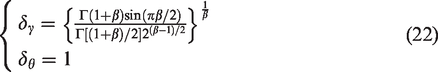
The schematic diagram of the two-dimensional plane Levy flight is shown in Figure 2.

Figure 2.

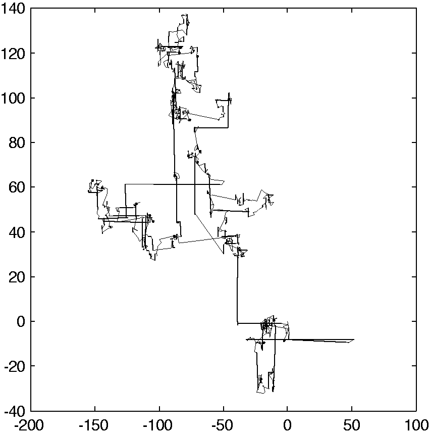
Levy flight trajectory.

The chick position based on the Levy mutation strategy is as follows

W_{i}^{j} (t + 1) = W_{i}^{j} (t) + B L * (W_{m}^{j} (t) - W_{i}^{j} (t))

(23)

The optimization process of the NCSO optimizer is shown in Figure 3.

Figure 3.

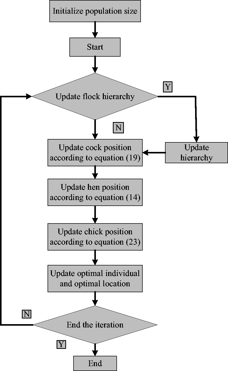
Optimization process.

Improved ELM

In the ELM model, connection weights and thresholds are chosen randomly. When the random weights and random thresholds are not appropriate, the calculation cost of the model will increase and the prediction accuracy of the model will be affected. In this study, the hyper parameters of the ELM model are optimized by the NCSO optimizer, and the power load is predicted by the NCSOELM model. The process of NCSOELM model predicting power load is shown in Figure 4.

Figure 4.

Predicting results. NCSOELM: ▪.

Figure 4 shows the forecasting process of the NCSOELM model:

Divide the sample set to determine the number of training samples and test samples.

Normalize load data.

The training sample is used to train the NCSOELM model. The NCSO optimizer optimizes the hyper parameters.

Test the NCSOELM model with the testing sample set.

Inverse normalization of predicted power load data.

NCSO optimizer test and power load forecasting

NCSO optimizer test

To test the optimization capability of the NCSO optimizer presented in this study, this section uses testing functions to test the convergence performance of NCSO and compare it with the CSO optimizer.

Four test functions are Sphere, Schwefel, Griewank, and Rastrigin functions (Li et al., 2019a, 2018a and Liu et al., 2019b). The values of the four function variables are [−100, 100], [−10, 10], [−600, 600], and [−5.12, 5.12]. The optimal values of test functions are all 0. The population size of NCSO and CSO optimizer is set as 20; the number of iterations is set as 500; the change frequency of hierarchy is set as 10. The dimension of the test function is set as 30 dimensions, and each function repeats the test for CSO optimizer and NCSO optimizer for 15 times, respectively.

The test results of NCSO and CSO optimizer are as follows.

By analyzing the convergence results of CSO optimizer and NCSO optimizer in Table 1, it is found that the convergence accuracy of NCSO optimizer is significantly higher than that of CSO optimizer. For the Rastrigin function, the CSO optimizer converges to the optimal value. But for the other three functions, the CSO optimizer does not converge to the optimal value. For Sphere, Griewank, and Rastrigin functions, the NCSO optimizer converges to the optimal value. For Schwefel function, compared with the convergence result of CSO optimizer, the convergence result of NCSO optimizer is closest to the optimal value.

Table 1.

Analysis of convergence results.

Function	Optimizer	Best value	Worst value	Average value
Sphere	CSO	1.01e-24	6.33e-17	4.81e-18
Sphere	NCSO	0	0	0
Schwefel	CSO	1.85e-21	1.75e-19	5.37e-20
Schwefel	NCSO	2.01e-220	2.35e-216	3.08e-217
Griewank	CSO	0	0.48	0.05
Griewank	NCSO	0	0	0
Rastrigin	CSO	0	5.48	0.36
Rastrigin	NCSO	0	0	0

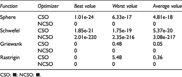
CSO: ▪; NCSO: ▪.

Because of the nonlinear dynamic convergence factor in the NCSO optimizer, the NCSO optimizer has stronger local and global convergence capabilities. The Levy mutation strategy can ensure the diversity of the population and enhance the ability of the population to jump out of the local optimum to a certain extent. To analyze the convergence capacity of the CSO optimizer and NCSO optimizer, Figure 5 plots the iterative curves of the two optimizers.

Figure 5.

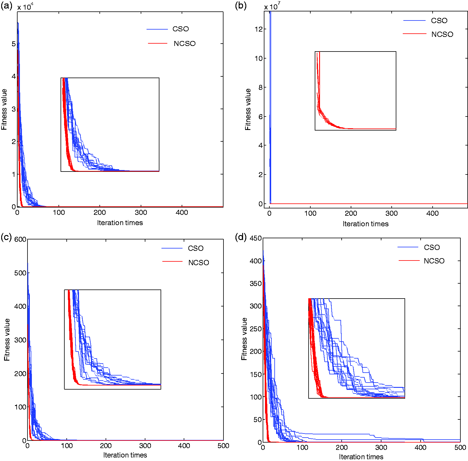
Iteration curve. (a) Sphere, (b) Schwefel, (c) Griewank, and (d) Rastrigin. CSO: ▪; NCSO: ▪.

As shown in Figure 5, for the four test functions, the NCSO optimizer’s iteration curve drops faster. The nonlinear dynamic convergence factor accelerates the convergence rate of NCSO optimizer. Compared with the iterative curve of NCSO optimizer, the convergence speed of the iterative curve of CSO optimizer is slower.

Power load forecasting based on NCSOELM model

The simulation data used in this paper comes from the sample data provided by the European intelligent technology network. In this paper, a week’s power load data are selected from the sample set for model training and testing. The power load data of a week include 336 samples, and the time series curve of the samples is shown in Figure 6.

Figure 6.

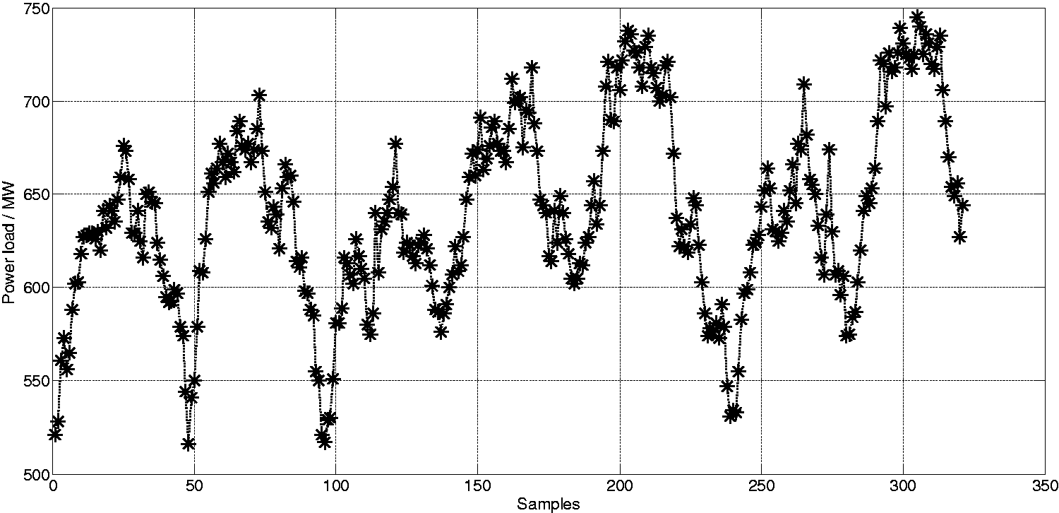
Power load time series curve.

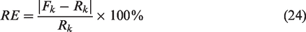
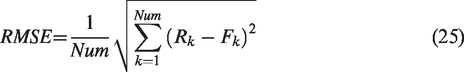
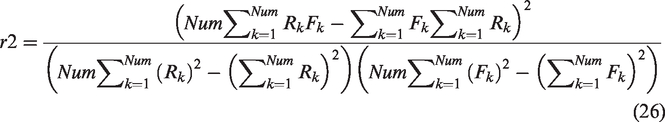
Relative error (RE) and root mean square error (RMSE) are used to evaluate the fitting error of the model. The determination coefficient (r2) is used to evaluate the fitting degree

R E = \frac{| F_{k} - R_{k} |}{R_{k}} \times 100 %

(24)

RMSE = \frac{1}{Num} \sqrt{\sum_{k = 1}^{Num} {(R_{k} - F_{k})}^{2}}

(25)

r 2 = \frac{{(Num \sum_{k = 1}^{Num} R_{k} F_{k} - \sum_{k = 1}^{Num} F_{k} \sum_{k = 1}^{Num} R_{k})}^{2}}{(Num \sum_{k = 1}^{Num} {(R_{k})}^{2} - {(\sum_{k = 1}^{Num} R_{k})}^{2}) (Num \sum_{k = 1}^{Num} {(F_{k})}^{2} - {(\sum_{k = 1}^{Num} F_{k})}^{2})}

(26)

where

Num

is the total number of samples,

R_{k}

is the sample value, and

F_{k}

is the sample prediction value.

First, the sample power load data of the first six days are used as the training sample, and the power load data of the last day are used as the prediction sample. The power load is predicted by the NCSOELM model on the seventh day and compared with the prediction results of the BP, SVM, and CSOELM models. The prediction results on the seventh day of each model are shown below.

The power load curve predicted by each model is shown in Figure 7(a). The four forecast curves all reflect the fluctuation trend of the true value curve. Figure 7(b) shows the REs of the four models. The prediction error distribution intervals of SVM model, BP model, CSOELM model, and NCSOELM model are [0.02%, 7.03%], [0.05%, 6.88%], [0.03%, 7.68%], and [0.15%, 6.61%], respectively. For one day’s power load prediction results, the RMSE and r2 values of the four forecasting models are shown in Table 2.

Figure 7.

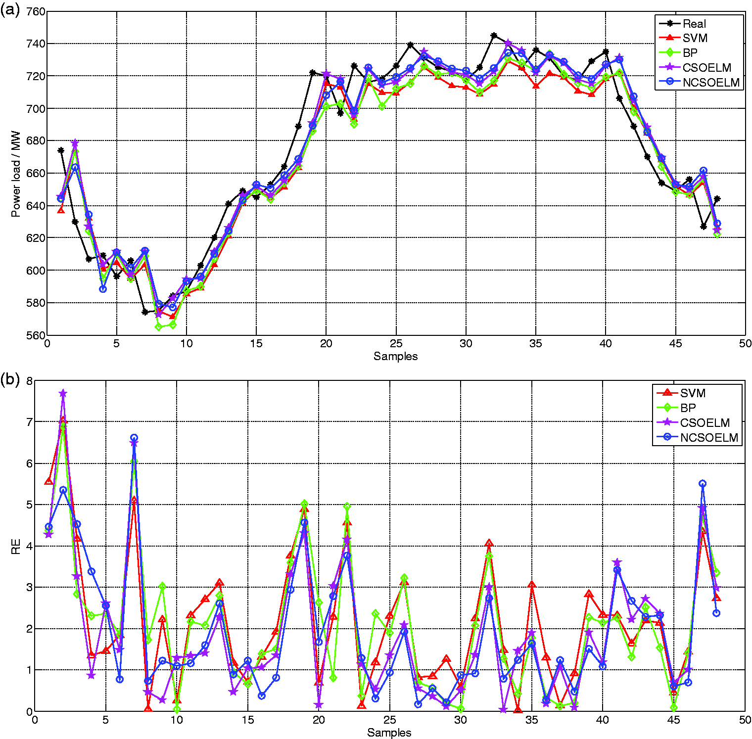
Power load forecasting results for one day. (a) Power load forecasting curve for one day and (b) RE of power load prediction for one day. BP: ▪; CSOELM: ▪; NCSOELM: ▪; SVM: support vector machine.

Table 2.

Predictive evaluation analysis.

Model	RMSE	r2 (%)
SVM	17.92	89.75
BP	17.50	90.04
CSOELM	16.61	90.14
NCSOELM	16.16	90.66

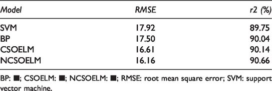
BP: ▪; CSOELM: ▪; NCSOELM: ▪; RMSE: root mean square error; SVM: support vector machine.

As shown in Table 2, the determination coefficient r² values of the four models areabout 90%. The highest r² value of the NCSOELM model is 90.66%, which indicates that the NCSOELM model has a better fitting degree. For the RMSE evaluation index, the minimum RMSE value of the NCSOELM model is 16.16 and the maximum RMSE value of the SVM model is 17.92, indicating that the forecasting errors of the NCSOELM model are smaller.

Second, the power load sample data from the first five days are used as the training set, and the power load data from the next two days are used as the prediction set. The SVM, BP, CSOELM, and NCSOELM models were used to forecast the power load for two days.

Figure 8(a) shows the forecasting curves. The forecasting curves can still reflect the changes of the two-day true value curves. Figure 8(b) shows the forecasting error curves. The RE fluctuation intervals of BP, SVM, CSOELM, and NCSEOLM models are [0.03%, 6.69%], [0.01%, 7.16%], [0.55%, 7.99%], and [0.01%, 6.66%], respectively. By comparing the error intervals, it can be found that the error interval of the NCSOELM model is smaller, which indicates that the NCSOELM model has higher forecasting stability.

Figure 8.

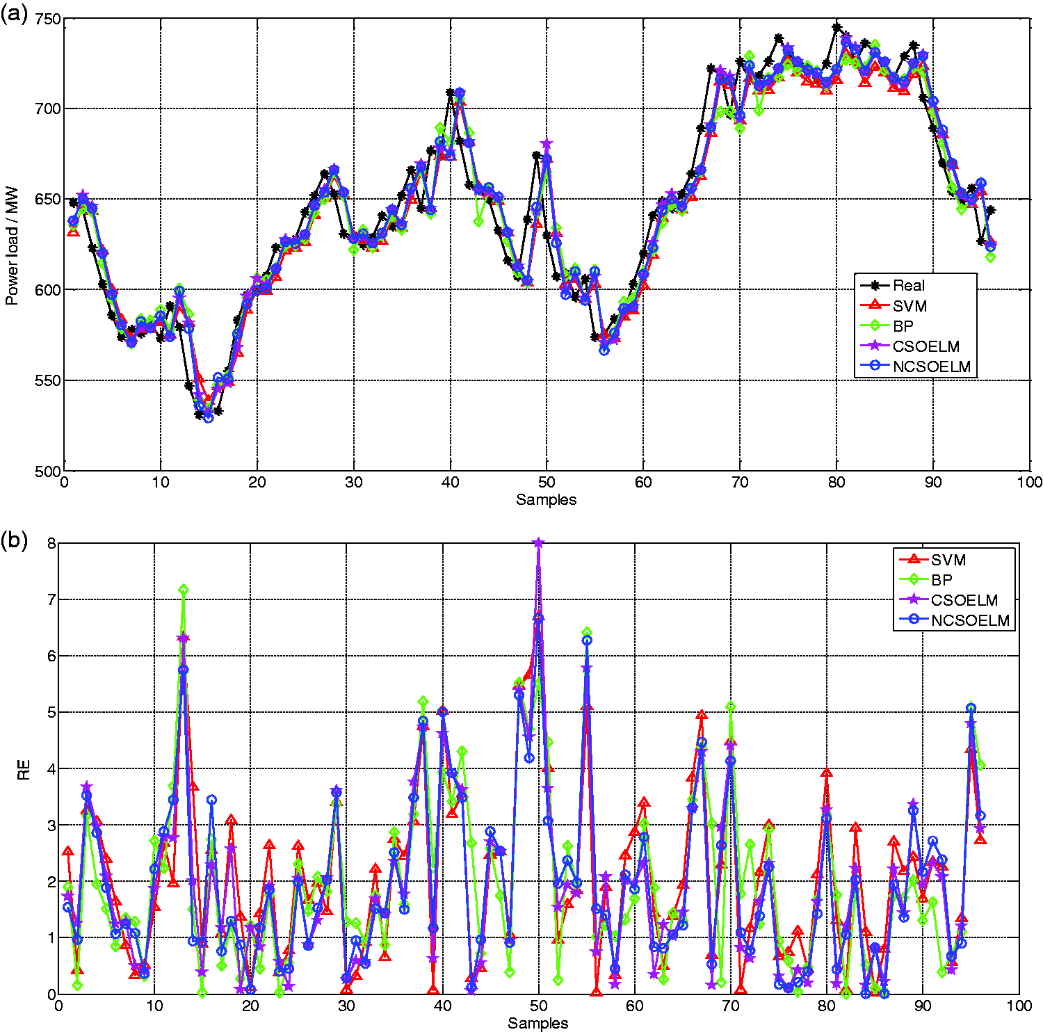
Power load forecasting results for two days. (a) Power load forecasting curve for two days and (b) RE of power load prediction for two days. BP: ▪; CSOELM: ▪; NCSOELM: ▪; SVM: support vector machine.

The results of the two-day power load forecast evaluation are shown in Table 3.

Table 3.

Forecasting results evaluation analysis.

Model	RMSE	r2 (%)
SVM	16.74	91.25
BP	16.28	91.60
CSOELM	16.12	91.57
NCSOELM	15.87	91.83

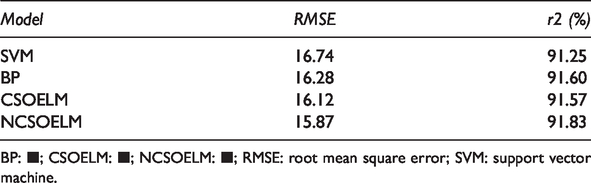
BP: ▪; CSOELM: ▪; NCSOELM: ▪; RMSE: root mean square error; SVM: support vector machine.

As shown in Table 3, the four models have achieved good fitting effect, and the determination coefficient r2 has reached 91%. Among them, the highest decision coefficient of NCSOELM model is 91.83%. The decision coefficients of NCSOELM are 0.58, 0.23, and 0.25% higher than those of SVM, BP, and CSOELM, respectively. For RMSE values, the RMSE value of the NCSOELM model is at least 15.87, and the RMSE value of the NCSOELM model is 0.87, 0.41, and 0.25 smaller than the RMSE values of the SVM, BP, and CSOELM models, respectively.

Conclusions

With the development of clean energy, electric power has become one of the most important clean energy. Electric energy has become a guarantee for the development of all walks of life. It is of great significance for energy system to mine the data of power load in the past. In order to promote the economic operation and development of energy system, NCSOELM model is proposed to predict the power load. By using the NCSOELM model to predict the power load of one day and two days, respectively, the following conclusions are obtained.

To improve the local and global search ability of CSO optimizer, the NCSO optimizer based on nonlinear dynamic convergence factor is proposed. And the levy mutation strategy is used in NCSO optimizer.

Compared with CSO optimizer, NCSO optimizer has faster optimization speed. For Sphere, Griewank, and Rastrigin functions, the NCSO optimizer converges to 0.

For one- and two-day power load forecasting, NCSOELM model shows high fitting effect and low prediction error. The decision coefficients of NCSOELM model are all above 90%. The RMSE value of the NCSOELM model is at least 15.87, and the RMSE value of the NCSOELM model is 0.87, 0.41, and 0.25 smaller than the RMSE values of the SVM, BP, and CSOELM models.

The economic operation of energy system can be realized by accurately forecasting the power load.

Footnotes

Declaration of conflicting interests

The author(s) declared no potential conflicts of interest with respect to the research, authorship, and/or publication of this article.

Funding

The author(s) disclosed receipt of the following financial support for the research, authorship, and/or publication of this article: This work was supported by the Natural Science Foundation of Hebei Province of China (Project No. E2018202282) and the key project of Tianjin Natural Science Foundation (Project No. 19JCZDJC32100).

ORCID iD

Ching-Hsin Wang

References

Abdel-Aal

(2004) Short-term hourly load forecasting using abductive networks. IEEE Transactions on Power Systems 19: 164–173.

Almuhtady

Alshwawra

Alfaouri

, et al. (2019) Investigation of the trends of electricity demands in Jordan and its susceptibility to the ambient air temperature towards sustainable electricity generation. Energy Sustainability and Society 9(1): 18.

AlRashidi

El-Naggar

(2010) Long term electric load forecasting based on particle swarm optimization. Applied Energy 87(1): 320–326.

Al Shayokh

Shin

(2017) Bio inspired distributed WSN localization based on chicken swarm optimization. Wireless Personal Communications 97(4): 5691–5706.

Amjady

Keynia

(2009) Short-term load forecasting of power systems by combination of wavelet transform and neuro-evolutionary algorithm. Energy 34(1): 46–57.

Bennett

Stewart

(2014) Autoregressive with exogenous variables and neural network short-term load forecast models for residential low voltage distribution networks. Energies 7(5): 2938–2960.

Bianco

Manca

Nardini

(2009) Electricity consumption forecasting in Italy using linear regression models. Energy 34(9): 1413–1421.

Buitrago

Asfour

(2017) Short-term forecasting of electric loads using nonlinear autoregressive artificial neural networks with exogenous vector inputs. Energies 10(1): 24.

Caro

Juan

Cara

(2020) Periodically correlated models for short-term electricity load forecasting. Applied Mathematics and Computation 364: 13.

10.

Cecati

Kolbusz

Rozycki

, et al. (2015) A novel RBF training algorithm for short-term electric load forecasting and comparative studies. IEEE Transactions on Industrial Electronics 62(10): 6519–6529.

11.

Ceperic

Baric

(2013) A strategy for short-term load forecasting by support vector regression machines. IEEE Transactions on Power Systems 28(4): 4356–4364.

12.

Cevik

Cunkas

(2015) Short-term load forecasting using fuzzy logic and ANFIS. Neural Computing & Applications 26(6): 1355–1367.

13.

Che

Wang

(2014) Short-term load forecasting using a kernel-based support vector regression combination model. Applied Energy 132: 602–609.

14.

Che

Wang

(2012) An adaptive fuzzy combination model based on self-organizing map and support vector regression for electric load forecasting. Energy 37(1): 657–664.

15.

Chen

Chang

Lin

(2004) Load forecasting using support vector machines: A study on EUNITE competition 2001. IEEE Transactions on Power Systems 19: 1821–1830.

16.

Chiu

Kao

Cook

(1997) Combining a neural network with a rule-based expert system approach for short-term power load forecasting in Taiwan. Expert Systems with Applications 13: 299–305.

17.

Erdogdu

(2007) Electricity demand analysis using cointegration and ARIMA modelling: A case study of Turkey. Energy Policy 35(2): 1129–1146.

18.

Espinoza

Joye

Belmans

, et al. (2005) Short-term load forecasting, profile identification, and customer segmentation: A methodology based on periodic time series. IEEE Transactions on Power Systems 20(3): 1622–1630.

19.

Essallah

Khedher

(2019) Comparative study of long-term load forecasting techniques applied to Tunisian grid case. Electrical Engineering 101: 1235--1247.

20.

Lin

, et al. (2019) Short-term wind power prediction based on improved chicken algorithm optimization support vector machine. Sustainability 11(2): 15.

21.

Huang

Ding

Zhou

(2010) Optimization method based extreme learning machine for classification. Neurocomputing 74(1–3): 155–163.

22.

Huang

Wang

Lan

(2011) Extreme learning machines: A survey. International Journal of Machine Learning and Cybernetics 2(2): 107–122.

23.

Huang

Zhou

Ding

, et al. (2012) Extreme learning machine for regression and multiclass classification. IEEE Transactions on Systems, Man, and Cybernetics Part B: Cybernetics 42(2): 513–529.

24.

Hyndman

Khandakar

(2008) Automatic time series forecasting: The forecast package for R. Journal of Statistical Software 27(3): 1–22.

25.

Kayacan

Ulutas

Kaynak

(2010) Grey system theory-based models in time series prediction. Expert Systems with Applications 37(2): 1784–1789.

26.

Lee

(2013) Short-term load forecasting using SVR (support vector regression)-based radial basis function neural network with dual extended Kalman filter. Energy 49: 413–422.

27.

Chen

Tseng

, et al. (2017a) Effective power management modeling of aggregated heating, ventilation, and air conditioning loads with lazy state switching. Journal of Cleaner Production 166(10): 844–850.

28.

Liu

Tseng

, et al. (2019a) Enhancing the Lithium-ion battery life predictability using a hybrid method. Applied Soft Computing 74: 110–121.

29.

Tseng

, et al. (2018a) Renewable energy utilization method: A novel insulated gate bipolar transistor switching losses prediction model. Journal of Cleaner Production 176: 852–863.

30.

Ren

Wang

, et al. (2017b) A new method to estimate the state of charge of the green battery. Microelectronics Reliability 79: 306–313.

31.

Sun

Wang

, et al. (2019b) Enhanced Gaussian process mixture model for short-term electric load forecasting. Information Sciences 477: 386–398.

32.

Yang

Tseng

, et al. (2018b) A novel method to solve sustainable economic power loading dispatch problem. Industrial Management & Data Systems 118(4): 806–827.

33.

Chen

, et al. (2015) Local binary patterns and extreme learning machine for hyperspectral imagery classification. IEEE Transactions on Geoscience and Remote Sensing 53(7): 3681–3693.

34.

Liu

Jin

Gao

(2019a) A new hybrid approach for short-term electric load forecasting applying support vector machine with ensemble empirical mode decomposition and whale optimization. Energies 12(8): 20.

35.

Liu ZF, Li LL, Tseng ML, et al., (2020a) Prediction short-term photovoltaic power using improved chicken swarm optimizer- Extreme learning machine model. Journal of Cleaner Production 248.

36.

Liu

Tseng

, et al. (2019c) Improving the reliability of photovoltaic and wind power storage systems using least squares support vector machine optimized by improved chicken swarm algorithm. Applied Sciences 9(18): 18.

37.

Meng

Liu

Gao

, et al. (2014) A new bio-inspired algorithm: Chicken swarm optimization. In: Tan

Shi

Coello

CAC

(eds) 5th International Conference on Swarm Intelligence, pp.86–94. Hefei: Springer International Publishing.

38.

Mirasgedis

Sarafidis

Georgopoulou

, et al. (2006) Models for mid-term electricity demand forecasting incorporating weather influences. Energy 31(2–3): 208–227.

39.

Mohan

Soman

Kumar

(2018) A data-driven strategy for short-term electric load forecasting using dynamic mode decomposition model. Applied Energy 232: 229–244.

40.

Pai

Hong

(2005) Support vector machines with simulated annealing algorithms in electricity load forecasting. Energy Conversion and Management 46: 2669–2688.

41.

Sharma

Ghosh

(2019) Effective design and development of hybrid ABC-CSO-based capacitor placement with load forecasting based on artificial neural network. Assembly Automation 39(5): 917–930.

42.

Tang

Dai

Wang

, et al. (2019) Short-term power load forecasting based on multi-layer bidirectional recurrent neural network. IET Generation, Transmission & Distribution 13(17): 3847–3854.

43.

Tiana

Zhanga

Lewandowskic

, et al. (2017) Deadlock-free migration for virtual machine consolidation using chicken swarm optimization algorithm. Journal of Intelligent & Fuzzy Systems 32(2): 1389–1400.

44.

Wang

(2016) An intuitionistic fuzzy sets-based hybrid approach to the innovative design evaluation mode for green products. Advances in Mechanical Engineering 8(4): 1–16.

45.

Wang

Tseng

Tan

, et al. (2017) Application of a mathematical programming model to solve the confidence interval. International Journal of Information and Management Sciences 28(1): 11–23.

46.

Zong

Huang

Chen

(2013) Weighted extreme learning machine for imbalance learning. Neurocomputing 101: 229–242.

Power load forecasting in energy system based on improved extreme learning machine

Abstract

Keywords

Introduction

Power load forecasting model

ELM model principle

Chicken swarm optimizer (CSO)

CSO based on nonlinear dynamic convergence factor (NCSO)

Improved ELM

NCSO optimizer test and power load forecasting

NCSO optimizer test

Power load forecasting based on NCSOELM model

Conclusions

Footnotes

Declaration of conflicting interests

Funding

ORCID iD

References