Sage Journals: Discover world-class research

Abstract

Pakistan pursued the renewable energy policy to minimize the cost of energy per kWh as well as dependence on costly imported oil. Jhimpir site is termed as wind corridor and has tremendous proven wind power potential. The site is hosted for the first installed wind power plant. The aim of paper is to investigate the performance and levelized cost of energy of a wind farm. The methodology covers assessment of wind characteristics, performance function and levelized cost of energy model. The measured mean wind speed was found to be 8 m/s at 80 m above the ground level. The average values of standard deviation, Weibull k and c parameters, obtained using entire data set, were found to be 2.563, 3.360 and 8.940 m/s at 80 m. Performance assessment including technical, real availability and average capacity factor was found to be 97, 90 and 34.50%, respectively. It is evident that the power coefficient dropped if wind speed crosses the rated power. So it can be concluded that the efficiency of wind turbine decreased by increased wind speed. Tip speed ratio shows that a wind turbine operating close to optimal lift and drag will exhibit the performance level. Wind turbine performs better at the wind speed between 6 and 10 m/s. The estimated average levelized cost of energy was US $0.11371 and US $0.04092/kWh for 1–10 and 11–20 years, respectively. This makes it competitive in terms of low production cost per kWh to other energy technologies.

Keywords

Wind characteristics Weibull parameters power coefficient tip speed ratio levelized cost of energy

Introduction

Energy inputs are significant for socio-economic development of a country. Wind energy can play a vital role in minimizing the dependence on oil, creating balance between supply and demand and less cost per kWh. From 1978 (Asif, 2009) to 2016 (Yearbook, 2016), Pakistan’s maximum energy consumption is given in Figure 1(a) and (b). There is no visible change realized in utilization of energy sources except rise in imported oil and natural gas. The oil, natural gas and coal consumption during 2015–2016 was up by 5.08, 6.53 and 3.6%, respectively (Yearbook, 2016). So in current scenario, reliance on oil is neither an economical nor environment friendly. Sudden rise in international oil prices directly hit the local economy. Natural gas is only abundant available indigenous source of energy but started to deplete owing to increased use during the last decade. The country’s largest National Oil and Gas Exploration Organization (OGDCL) predicted that local oil and natural gas reserves expected to be deplete in 2025 and 2030, respectively (Sheikh, 2010). According to energy book 2016 of Hydrocarbon Development Institute of Pakistan, the balance recoverable reserves of indigenous energy source oil and natural gas were 47.04 and 330.27m tons of oil equivalent (TOE), respectively. Oil production dropped down 8.5% in 2015–2016 while natural gas slightly moved up 0.8% in 2015–2016 (Yearbook, 2016). Figure 1(a) and (b) is showing the share of each source of energy utilization in 1978 and 2016.

Figure 1.

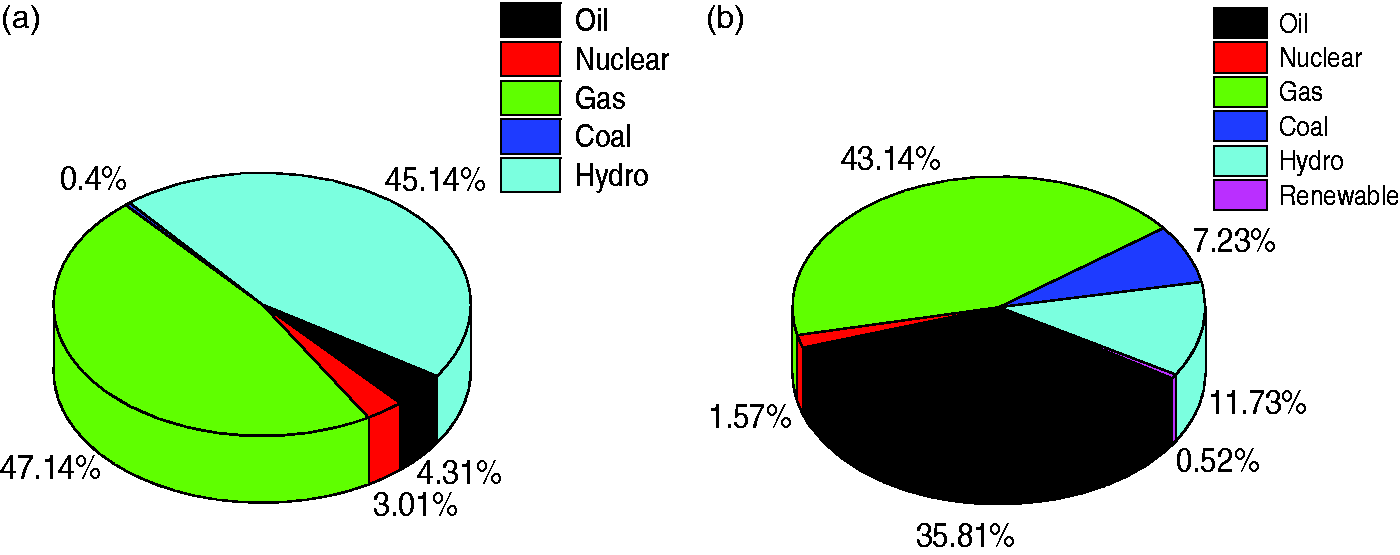
Energy resources utilization (%). (a) 1978 (Asif, 2009) and (b) 2016 (Yearbook, 2016).

Pakistan has a considerable wind potential at the coastal belt. Pakistan Meteorological Department (PMD) collected wind data by installing wind mast at different parts. The wind mapping of Pakistan was also prepared by National Renewable Energy laboratories (NREL). Pakistan has 68,863 km² appropriate windy land that accounts for 9.06% of total land (Shami et al., 2016). The Government of Pakistan established an Alternative Energy Development Board (AEDB) in 2003 to set long- and short-term objectives for renewable energy. With the objective of renewable energy to minimize the ever increasing effect of tariff (Eberhard and Kåberger, 2016; Meneguzzo et al., 2016), Jhimpir site is selected as a first site for installation of wind energy power plants.

There are number of research studies available in the literature of wind turbine performance contextualizing the models under the frame work of traditional wind models (Bezrukovs et al., 2016; Gao et al., 2016). The study of wind turbine performance is less prominent to on site information as opposed to the modelling of wind turbine performance (Wang et al., 2016). For instance: the random wind speed (m/s) variation is a significant characteristic of the site as well as a prominent feature of wind turbine performance (Shu et al., 2015). The wind turbine performance can be declined by increased wind loads (Cooney et al., 2017; Ganjefar and Mohammadi, 2016; Petković et al., 2013; Shahizare et al., 2016) that lead to failure of components (Faulstich et al., 2011; Nejad et al., 2014). The wind turbine field investigation characterized as the time consuming due to large number of data. This form of disparagement can relatively be considered as a well-meaning for the assessment being presented in this paper. The variation in wind speed is an important characteristic of site and is therefore an imperative factor of wind turbine performance.

The economics of wind energy is another fundamental concern for the renewable energy (Hemmati, 2017). The studies presented in the literature simply focused on the life cycle assessment of wind energy (Wang and Teah, 2017) or its capital intensive nature (Kanyako and Janajreh, 2015) or describing the capital costs of wind turbine and grid connections that can only accounts for the 80% of the total costs (Blanco, 2009). But the real essence of performance and energy economics of per kWh is depends on the wind conditions of the site. The financial effect of wind energy technology in terms of network costs increased due to population density that focused on the expenses being spent on the cable required for per consumer assessed (O’Flaherty et al., 2014). The increasing trend of wind power generation, as an additional source of energy, is gaining strength but one of difficulty related with the wind energy is determining the suitable site. Detailed methods including geometric data and aerodynamic performance are required to ascertain potential site (Millward-Hopkins et al., 2013). The site-specific wind characteristics-based wind machines should be designed as proposed by Toft et al. (2016) and Amar et al. (2008). Similarly, the effect of wind variation leads to decreased power generation (Dokopoulos et al., 1996). Wind is random variable and changes over a period of time. The fluctuating nature of wind had substantial effect on voltage, frequency and performance (Sørensen et al., 2001).

There are two widely accepted assumptions for decreased performance function of wind turbines. One is the failure of components that leads to halt down of wind turbine operations. The other is repair and replacement activity for restoration of system. The failure of components resulted into decreased operation time, cost of replacement and maintenance (Carroll et al., 2015). The survey statistics of various European wind farms showed that the failure and maintenance of wind turbine components lead to reduced performance (Le and Andrews, 2015) and (Ribrant and Bertling, 2007). The performance assessment of Muppandal, Tamil Nadu wind farm presented by (Herbert et al., 2010). The author concluded that the performance of wind farm is affected by immature failure of electrical and mechanical components and presented spare parts focused strategy. Wind characteristics can be a source of increased fatigue loads and decreased life of wind turbine components (Veers and Winterstein, 1998). In some studies, the preventive maintenance-based approaches used to improve the performance of wind farm (Igba et al., 2015; Nilsson and Bertling, 2007; Puglia et al., 2014).

Monte Carlo-based Markov chains modelling used for estimating capacity factors of wind farms (Gurgur and Jones, 2010). The performance modelling of wind farms based on the experimental data of wind turbines ranging from 20 to 1650 kW used to predict the performance function (Bhatt and Jothibasu, 2002). The performance of wind turbines can be improved by additions of new materials and technologies (O’Dell, 2001). The performance of wind turbines can be improved if spacing between the wind turbines is minimized (Ammara et al., 2002). Similarly, the wind uncertainty based risk-related energy generation has been examined by (Şen, 1997) and (Yang et al., 2003). The capacity factor is an effective tool used to determine the wind turbine performance ((Mejía et al., 2006) and efficiency interdependence between energy generation and wind speed (Lai and Lin, 2006).

The prediction-based performance models have been used to present the operational considerations of wind turbines (Yang et al., 2016). This is an important characteristic while considering the performance forecasting as well as monitoring. The power curve-based new parametric models considering the modified hyperbolic tangent proposed to characterize the wind turbine (Wang et al., 2016) and machine learning-based approach presented for modelling the behaviour of wind turbine (Marvuglia and Messineo, 2012). These non-parametric models can provide the reasonable performance outcome based on pre-processing information.

From an economical point of view, the rising trend of installation of wind power plants noticeably associated with the reduction of energy cost (Boubault et al., 2016). As an industry permanence, cost of components and large applicability is driving factors for levelized cost of energy (LCOE) (Parrado et al., 2016; Starke et al., 2016). The LCOE method is superior to the NPV method owing to its applicability in large projects. The net present value (NPV) is defined as difference between the present value of cash inflows and the present value of outflows for over period of time. NPV cannot be compared between projects either difference in scale or technology. NPV relies heavily upon multiple assumptions and estimates, so there can be substantial room for error. The LCOE method is used to compare different power generation equipments and technologies. Simply NPV is not feasible method to make prior choices between the projects (Zhao et al., 2017). The LCOE method is proposed in this paper. The LCOE method is not only presented as an economic characteristic but also as a scientific parameter by taking into account the additional valuable characteristics including performance function, availability function, aging, power correction factor, operation and maintenance (OM), wind power yield (kWh/m²/year), costs and life time.

The abovementioned literature focused on survey cum failures, maintenance, addition of materials and technologies, life cycle cost assessment and predictive models. The non-parametric models can provide the reasonable performance outcome but needs the pre-processing information. Similarly, the survey reports of wind farm just focused on the failure statistics of wind turbine components. However, there is little importance given to on site assessment of wind turbine performance and its ability to cope wind variations of practical site. Wind farm field experiments quantified as time consuming due to large number of data. This form of criticism can relatively be considered as the worthy for this analysis being presented in this paper. So, the gap is covered by incorporating on site performance of wind farm consists of real and technical availability, capacity factors, power coefficient, tip speed ratio and at what wind speed, the wind turbine operates efficiently. The performance-based LCOE economic model is proposed to calculate the cost/kWh as a scientific parameter. For the proposed model calculation, the energy generation benchmark set 142 GWh for the wind farm life time of 20 years. The wind farm energy generation and LCOE showed a significant impact of energy and cost per kWh on consumers.

Site description and local wind data measurement

Jhimpir is a small village of Thatta district of Sindh, province of Pakistan. Pakistan’s first selected site for installation of wind power plant is properly located at 120 km north east of the Karachi. The site is 3–5 m above the sea level. The wind speed measurements were taken at 10 minutes interval for the period of a year 2012. The geographical location of Jhimpir site is 25° 03' 58.50”N and 67° 58' 03.10”E. The terrain is simple and has no major obstacles. Also, similar terrain was found in west, north and south but east has some agricultural land. The site is geographical connected to the Karachi and Hyderabad, major cities of Pakistan. Figure 2 presents the wind farm.

Figure 2.

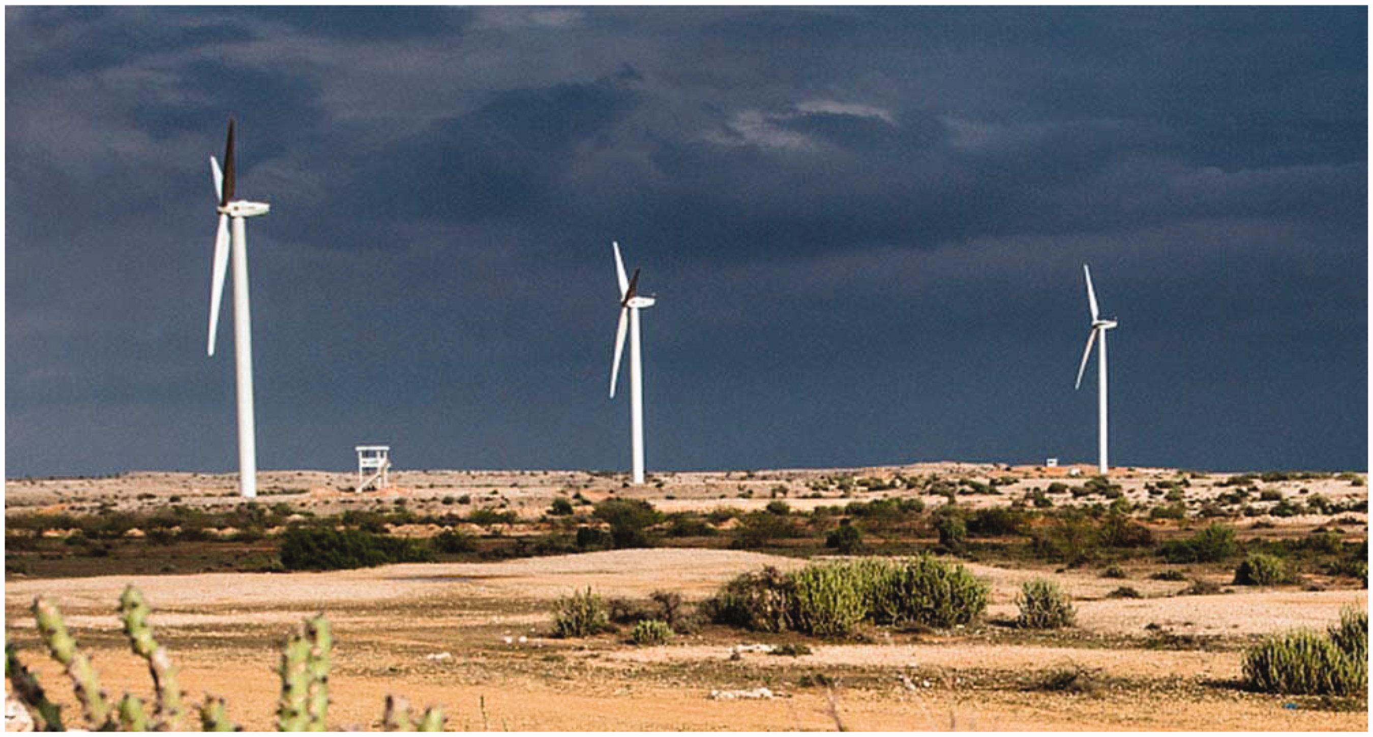
Wind farm site Jhimpir, Pakistan.

Methodology

The methodology covers the assessment of wind characteristics of site. The wind data are obtained at 10 minutes interval for the period of a year. The wind speeds and direction were measured at the 80 m above the ground level (AGL). The wind data have been used to analyse the performance characterization of prevailing wind conditions at the wind farm site for a period of a year. The measurements taken of wind direction and speeds are potential elements which have been considered in this study. This detailed measured information can be utilized for the future wind farm site analysis. The wind farm performance is analysed and discussed with reference to the wind characteristics and expected performance. The objective of this analysis is used to determine the impact of the wind environment on the anticipated efficiency and operation of the wind farm.

Wind characteristics and Weibull distribution functions

Wind is the random variable and highly fluctuating meteorological parameter that changes with time of the day, day of the year and year to year. The probability distribution function (pdf) can be calculated for changing nature of wind over a period of time. The wind speed can be measured by Weibull distribution function. Probability density function $f (v)$ can be expressed as (Akpinar and Akpinar, 2005)

f (v) = (\frac{k}{C}) {(\frac{V}{C})}^{k - 1} exp [{(- \frac{V}{C})}^{k}]

(1)

where V refers to wind speed, k refers to shapeless parameter and c refers to scale parameter having similar dimension of wind speed V. The cumulative distribution function (CDF)

f (v)

is given below (Akpinar and Akpinar, 2005)

f (v) = 1 - e x p [{(- \frac{V}{C})}^{k}]

(2)

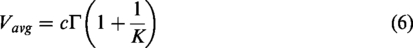
Mean wind speed is used to measure potential of wind energy generation which can be expressed as $V_{m e a n}$ . It can be calculated as given in Akpinar and Akpinar (2005) and the wind speed variance $σ^{2}$ can be expressed as follows (Akpinar and Akpinar, 2005)

V_{m e a n} = \frac{1}{N} {\sum_{i = 1}^{N} V}_{i}

(3)

σ^{2} = \frac{1}{N - 1} \sum_{i = 1}^{N} {(V_{i} - V_{a v g})}^{2}

(4)

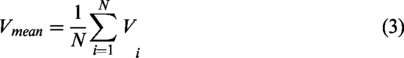
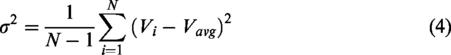
The standard deviation can be calculated as

σ = \sqrt{\frac{1}{N - 1} \sum_{i = 1}^{N} {(V_{i} - V_{a v g})}^{2}}

(5)

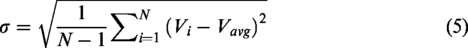
The mean and variance of wind speed can be calculated by Weibull parameters (Keyhani et al., 2010)

V_{a v g} = c Γ (1 + \frac{1}{K})

(6)

σ^{2} = C^{2} [Γ (1 + \frac{2}{K}) - Γ^{2} (1 + \frac{2}{K})]

(7)

Here, $Γ$ is the gamma function and can be solved by the following formula

Γ (X) = \int_{0}^{\infty} e^{- μ} u^{x - 1} du

(8)

Further, the maximum likelihood (ML) method can be used to determine the Weibull parameters k and c. The shape k and scale c parameters are calculated as follows

k = {[\frac{\sum_{i = 1}^{N} {V_{i}}^{K} l n (V_{i})}{\sum_{i = 1}^{N} {V_{i}}^{K}} - \frac{\sum_{i = 1}^{N} ln (V_{i})}{N}]}^{- 1}

(9)

c = {(\frac{1}{N} \sum_{i = 1}^{N} {V_{i}}^{k})}^{\frac{1}{K}}

(10)

where N is the number of wind speed data points;

V_{i}

is the wind speed value for the i-th data measurement.

Wind farm performance analysis model

In this section, the wind turbine performance assessment is examined. The power achieved from wind can be expressed as (Petković et al., 2013)

P_{W} = \frac{1}{2} ρ A_{T} V^{3}

(11)

where

ρ

refers to air density,

A_{T}

refers to swept area of blade and

V^{3}

refers to wind speed. According to Betz theorem that only less than 16/27 of the kinetic energy can be converted to mechanical energy. The Betz coefficient is denoted by

C_{p}

which can be expressed as (Schlechtingen et al., 2013)

P = \frac{1}{2} ρ C_{p} A_{T} V^{3}

(12)

The wind power density with Weibull probability density function can be calculated as follows (Ucar and Balo, 2009) and the wind energy obtained from the chosen wind turbine can be calculated using equation (12) (Petković et al., 2013)

W P D = \frac{P}{A} = \frac{1}{2} ρ C_{p} V^{3}

(13)

E = T \int_{0}^{\infty} P (V) . f (V) d (V)

(14)

where E refers to energy obtained, T refers to time period and P(V) refers to power curve of wind turbine. Substitute values of equation (4) in equation (12), we can find the following equation

E = T \int (\frac{k}{C}) {(\frac{V}{C})}^{k - 1} e x p {(- \frac{V}{C})}^{k} . p (V) d (V)

(15)

The above equation is the Weibull distribution function for achieving the wind energy.

Capacity factor

The capacity factor is an effective tool used to determine the wind turbine performance and efficiency. The capacity factor can be expressed as

c f = \frac{A c t u a l p o w e r f r o m w i n d t u r b i n e}{R a t e d p o w e r o f w i n d t u r b i n e}

(16)

Power curve analysis

Power curve estimation can be expressed by following equation (Cooney et al., 2017)

A_{E O} = (365 \times 24) (0.5) . ρ . A . \int_{0}^{\infty} C_{p} (λ) . p (V) V^{3} d (V)

(17)

where

A_{E O}

refers to total annual energy output is calculated to be kWh based on the power curve.

Power coefficient

Power coefficient ( $C_{p}$ ) is referred as a ratio of achieved power to an available power that can be expressed as (Pelletier et al., 2016)

C_{p} = \frac{P}{\frac{1}{2} . ρ . A_{T} . V^{3}}

(18)

Tip speed ratio

Tip speed ratio $(λ$ ) is referred as a ratio of the rotational velocity of blade tips over wind speed (m/s) that can be expressed as (Shahizare et al., 2016)

λ = \frac{ωR}{V}

(19)

where

ω

refers to rotational speed and R refers to the radius of wind turbine.

Availability factor analysis

Availability factor is extreme up to 100% and can be expressed as

A v a i l a b i l i t y = \frac{N e t D e l i v e r d E n e r g y + L o s t E n e r g y}{W i n d f a r m p o w e r c u r v e}

(20)

LCOE model

The LCOE is equal to the sum of all costs incurring during the lifetime divided by the units of energy generated during the lifetime. The LCOE set parameters including availability 97%, power curve density correction factor 5%, electrical losses 2.5%, auxiliary consumption 1%, air density 1.225 kg/cm⁻³; loan repayment is 10 years, and 17% on the return on equity for a period of 20 years. This is the most important approach to use the life cycle cost method that can be preferred over NPV. The LCOE ( $L_{c o e}$ ) of wind power plant installed in a year t can be expressed as

L_{c o e} (t) = (\frac{(T_{c}) + (L_{c}) + \sum_{i = 1}^{T} [\frac{(T_{c}) (O_{M} + I)}{{(1 + d)}^{i}}]}{\sum_{i = 1}^{T} [\frac{W C_{f} η {(1 + D_{r})}^{i}}{{(1 + d)}^{i}}]})

(21)

where

T_{c}

refers to the total cost of wind power plant, L refers to the cost of the land, I refers to the insurance cost (%),

O_{M}

refers to the OM cost, W refers to the wind power yield (kWh/m²/year),

η

refers to the availability factor (%) of the wind power plant,

C_{f}

refers to power correction factor (%) and T refers to the life time of the wind power plant. The LCOE calculation represents for a period of a year. For LCOE, the valuable variables are total cost of wind power plant

T_{c}

, wind power yield (kWh/m²/year) and availability factor of the wind farm. However, the cost of the wind power plant at certain time (

T_{c}

) based on the cumulative installed capacity of wind power.

Results and discussion

Wind characteristics of site

Wind speed

Wind is the random and highly fluctuating meteorological parameter that changes with time of the day, day of the year and year to year. The mean-measured wind speeds were found to be 8 m/s at 80 m AGL. It is notable from the measured wind data that there is significant variation present throughout the period of a year as shown in Figure 3(b). Figure 3(a) displays the fluctuation of wind measurement taken at 80 m for a period of 24 hours.

Figure 3.

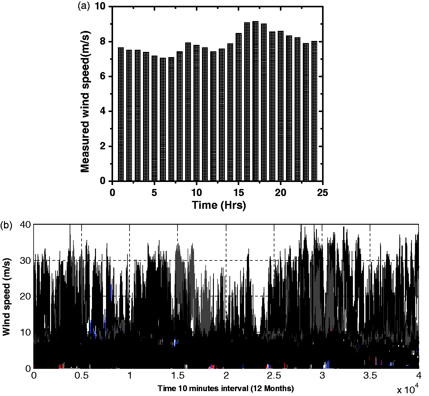
Measured wind speed (m/s) of site for (a) 24 hours a day and (b) for 10 minutes interval for a year.

Wind direction

Figure 4 displays the wind speed rose data obtained at 80 m of wind turbine. The wind rose contains the details of prevailing wind direction of which preliminary comes out from a range of south–south easterly (SSE) to south–south westerly (SSW) direction with a significant section of wind blowing from south easterly–westerly direction. Figure 4 contains the information of wind rose of 24 hours a day and frequency of different wind speeds denoted corresponding direction.

Figure 4.

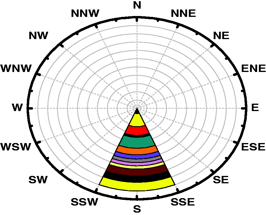
Wind rose graph of wind farm site.

Weibull distribution function

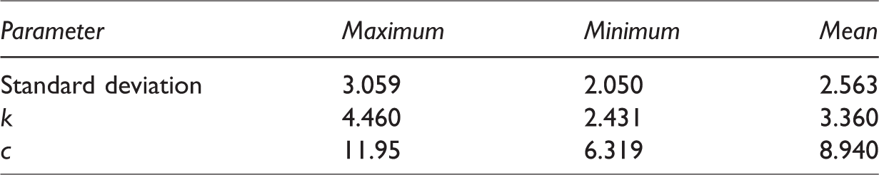
The average values of standard deviation, Weibull k and c parameters, obtained using entire data set were found to be 2.563, 3.360 and 8.940 m/s at 80 m (AGL).The seasonal values of shape parameter were found to be 2.525, 3.650, 3.904 and 3.357 during winter, spring, summer and autumn, respectively. The highest value of shape k parameter was found to be 3.904 during the summer and lowest 2.525 in winter. The highest value of scale c parameter was found to be 10.11 m/s and minimum 6.932 m/s in summer and winter time, respectively. The seasonal calculation showed variation over a period of time. The higher values of standard deviation were found to be 2.673 and lower 2.472 in autumn and spring, respectively. Figure 5(a) and (b) presents the calculated values of standard deviation and Weibull k and c parameters using entire data set for a period of year. The results of standard deviation and Weibull distribution parameters k and c at 80 m are summarized in Table 1.

Figure 5.

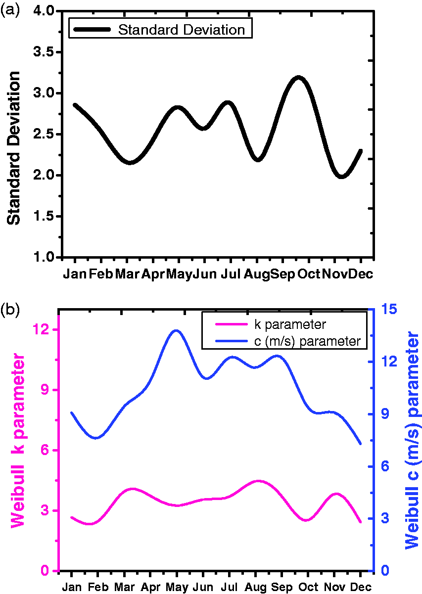
Site-specific values of (a) standard deviation and (b) Weibull k and c (m/s) parameters for a period of a year.

Table 1.

Weibull parameters k and c (m/s) and standard deviation (σ) of wind farm site for a period of year.

Parameter	Maximum	Minimum	Mean
Standard deviation	3.059	2.050	2.563
k	4.460	2.431	3.360
c	11.95	6.319	8.940

Frequency distribution of wind

Frequency distribution analysis has been carried out to enable further observation of wind resource available at site over a period of time. The frequency distribution of site showing the dominant wind speeds. The distribution of wind speed within the limit has important implications on the performance characteristics of wind turbine. However, it is generally concluded from the measured wind speed data of wind farm site that the most of wind speed found below the cut out wind speed (25 m/s) of wind turbine. As a result, the generator output can only attain maximum power capacity of 2.0 MW. Weibull distribution is also used to estimate the total occurrence of each wind speed throughout the period so that yearly energy output and capacity factor can be predicted and compared with the measured data. Figure 6 displays the frequency of occurrence of wind speed of wind farm site.

Figure 6.

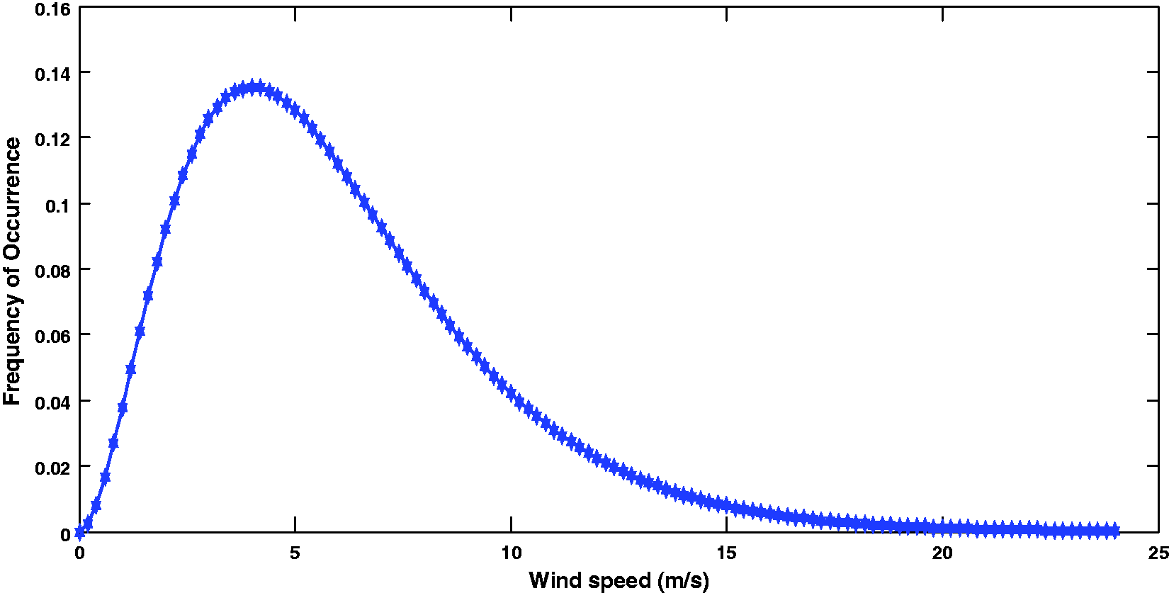
Frequency of occurrence of wind speed (m/s).

Performance analysis model

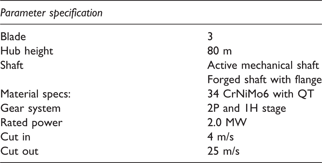
The performance model of wind power plant is studied under the following heads. However, the installed capacity of wind farm is 56.4 MW. There are 28 wind turbines installed at 80 m AGL. The mean wind power density (W/m²) and energy density (kWh/m²) were found to be $599 W / m^{2}$ and $1376 {k W h / m}^{2}$ at 80 m, respectively. It is also noted from the available wind speed data that the wind power density and energy yield during the summer season (June to August) comparatively higher than the other seasons. The features of wind turbine are summarized in Table 2.

Table 2.

Technical specification of wind turbine.

Parameter specification
Blade	3
Hub height	80 m
Shaft	Active mechanical shaft
Shaft	Forged shaft with flange
Material specs:	34 CrNiMo6 with QT
Gear system	2P and 1H stage
Rated power	2.0 MW
Cut in	4 m/s
Cut out	25 m/s

QT: Quneched.

Power curve analysis

The International Electro technical Commission (IEC) 61400–12 describes the power curve as important measure of wind turbine performance. The analysis of wind power curve conversion capabilities with fluctuating wind speed is important for observing the variation in power capabilities of wind turbine which causes the financial loss (Schlechtingen et al., 2013). In this study, the wind farm power conversion capabilities on site scenario are taken into account to assess the variation in power generation owing to continuously changing wind speeds. Also, this study can present the real operational case of wind farm, which is necessary to compare with the manufacturer stated wind power to wind farm power curve. The manufacturer’s stated power curve of wind turbine and wind farm is given in Figure 7. The power curve exhibits the behaviour of wind turbine along with peak output of 2.0 MW.

Figure 7.

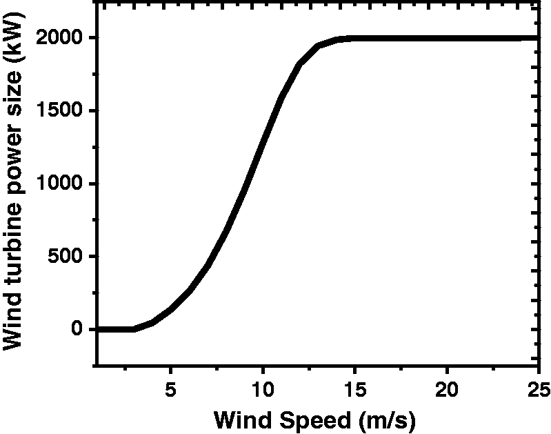
Manufacturer stated wind turbine power curve.

This paper is based on the real operations of wind farm so it is indispensable to compare the manufacturer stated power curve to wind farm power curve. Figure 8 represents the power curve data obtained from the wind farm is akin to expected performance and also emblematic shape of wind power curves as described in many studies (Pelletier et al., 2016; Petković et al., 2013; Wang et al., 2016). However, there is noteworthy difference presented between the mentioned studies. The power output measured at different wind speeds is greater than the manufacturer stated wind turbine power curve. Figure 8 displays the power output at different wind speeds (m/s) is higher than the stated by manufacturer for a period of month.

Figure 8.

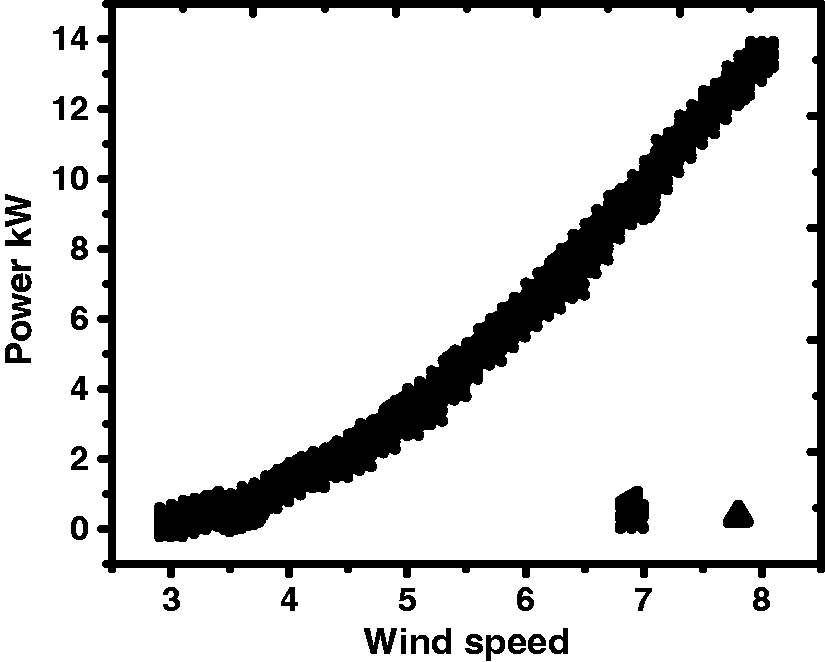
Wind turbine power curve based on measured data.

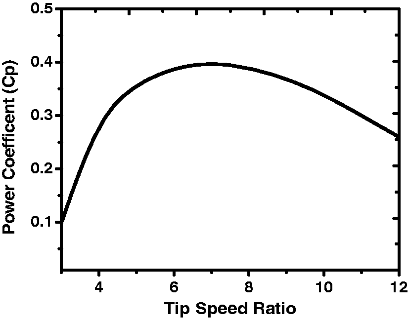
Power coefficient

Power coefficient is an important parameter as it describes the wind turbines aerodynamics efficiency in converting kinetic energy into electrical energy (Cooney et al., 2017; Shahizare et al., 2016). Betz limit sets highest value of 0.59 on the power coefficient value associated with wind turbine. However, the power coefficient ranges from 0.30 to 0.45 can be expected for a wind turbine working in real situation. Figure 9 shows the behaviour of power coefficient against the wind speed with efficiency peaking when wind speed is in between 6 and 10 m/s. However, it is obvious from the power coefficient that if wind speed crosses the rated power, the power coefficient is dropped. So it can be concluded that the efficiency of wind turbine is decreased with increased wind speed. The wind turbine operates efficiently between 6 and 10 m/s. This is evident that the wind turbine suited to 6–10 m/s wind speed, if the wind speed (m/s) increases beyond, the power coefficient dropped significantly.

Figure 9.

Power coefficient Cρ Versus wind speed (m/s) for 2.0 MW rated wind turbine based on wind farm measured data.

Tip speed ratio

Tip speed ratio and power coefficient affiliation are discussed as an indicator of performance. The tip speed ratio was found in between 2 and 12. Figure 10 showing the tip speed ratio which is different from many found in the literature that exhibits a slow drop off of a power coefficient post peak (Ganjefar and Mohammadi, 2016; Petković et al., 2013). However, it showed that the wind turbine operating close to optimal lift and drag will exhibit the performance level.

Figure 10.

Tip speed ratio λ vs. power coefficient Cρ for 2.0 MW wind turbine based on wind farm measured data.

Figure 11 displays the relationship of power coefficient and tip speed at different wind speeds (m/s). Figure 11 indicating the effect of dominant wind speeds on the performance of the wind turbines. This is essential determining factor for selection of wind turbine for a particular wind site. Figure 11 also shows the wind turbine performs better at the wind speed between 6 and 10 m/s.

Figure 11.

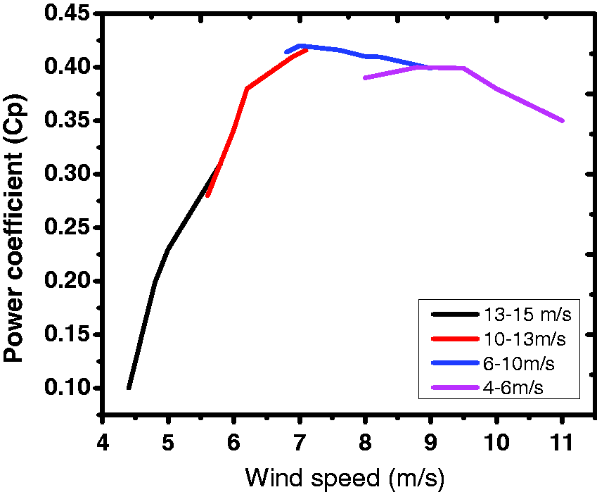
Power coefficient versus tip speed ratio for wind turbine at different wind speeds (m/s).

Availability factor analysis

Technical availability factor of Jhimpir wind farm was found to be 97% for a period of two years (2014 and 2015), respectively. Real availability factor of Jhimpir wind farm was found to be 93 and 90% in first and second year, respectively. The real availability of wind farm falls short because wind turbine did not operate total time. The real availability of wind farm decreased owing to increased number of failure of components, replacement, maintenance, grid loss, distribution loss and low wind. Wind farm operated for 1944.2 and 2102.4 hours in first and second year out of 17,520 hours. The average availability time of wind farm was found to be 22.20 and 24% for first and second year, respectively. The real availability of wind farm was increased in the second year. Figure 12 is showing the energy production (Ep), low wind (LW) and grid loss (GL) time was found to be increased in the second year compared to the first year. Similarly, the distribution network loss time and voltage Dip time were found to be decreased in the second year compared to first year. However, the mechanical loss (ML) and electrical components loss (EL) time showed the increasing tendency of failures that was the significant contributing factor of reduced real availability of wind farm.

Figure 12.

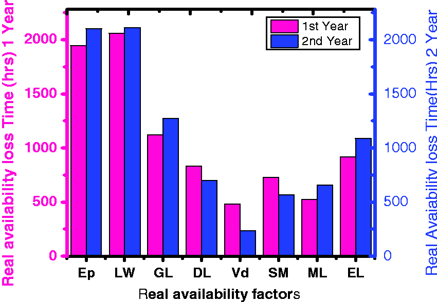
Comparison of real availability factors loss time for a period of two years.

Measured data

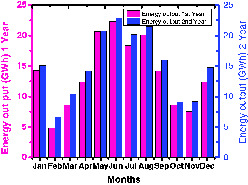
In order to calculate the total energy converted by the wind turbine, the sum total of measured power acquired at the 10 minutes interval was divided by the number of samples acquired to obtain an average power output. This was then multiplied with the number of available hours in year to obtain the total energy produced by the wind turbine. The total energy output was found to be 164.4 and 180.8 GWh in first and second year, respectively. There was increase of 16.4 GWh of energy noticed in second year of operations compared to first year. The average energy production was found to be 172.6 GWh. The energy production time found to be 22.2 and 24% of the overall time during first and second year, respectively. The energy generated was found to be 15.5 and 22.10% higher during the first and second year than the set benchmark 142 GWh. This shows that there was a significant increase of performance in terms of increase in energy generation in second year of operations compared to first year. In general, the wind farm showed an increase in energy output compared to energy set benchmark. Figure 13 showing the average energy generation during the summer season was higher than the other seasons. During the summer season, the flow of wind speed (m/s) at wind farm site is higher than other seasons. The monthly energy produced during the period of two years is given in Figure 13.

Figure 13.

Energy output of wind farm for a period of two years period.

Capacity factors

The capacity factors are effective and commonly used as a metric for the overall performance and efficiency of a wind turbine. The capacity factor was found to be 32.80 and 35.50% in first and second year, respectively. The average capacity factor for a period of two years was found to be 34.15%. This is very promising value for the installed wind turbine at Jhimpir wind farm that indicates the initial capital costs should be recuperated. The capacity factors of the measured data raise the possibility of improvements in the operational efficiency of the wind farm. The capacity factor of the wind turbine can be improved by forecasting, sitting techniques and introduction of smart grid systems allowing the higher amount of electricity available to the grid. The capacity factor for a period of a year is summarized in Table 3.

Table 3.

Measured capacity factor for a period of a year.

Months	Jan	Feb	Mar	Apr	May	Jun	Jul	Aug	Sep	Oct	Nov	Dec	Mean
C f (%)	30	20	33	39	54	42	48	32	48	32	30	18	35.50

LCOE model

A reasonable estimation of OM costs lies between 0.01 and 0.02/kWh (Blanco, 2009). The LCOE has been calculated for a life time (20 years) of wind turbine based on a range of OM cost predictions. According to (Neuteleers et al., 2017), setting of tariff for intermittent nature of renewable energy is highly complex. In this paper, the tariff model presented is based on set bench mark of energy production summarized in Table 4 which minimizes the complexity. Table 4 contains the costs of OM, insurance, return on equity, WH tax, loan repayment and interest charges. The LCOE was calculated for life time (20 years) of wind farm. The bench mark set for LCOE is 142 GWh energy produced by wind farm in a year.

Table 4.

Levelized tariff and cost of energy (US$/kWh) for life time of 20 years.

Year	O & M		Insurance	ROE	WH tax (%)	Loan payment	IR (%)	Total
Year	Variable	Fixed	Insurance	(%)	WH tax (%)	Loan payment	IR (%)	Total
First	0.00059	0.0069	0.0049	0.025	0.0018	0.043	0.0033	0.0855
Fifth	0.00059	0.0069	0.0049	0.025	0.0018	0.055	0.0220	0.1162
10th	0.00082	0.0084	0.0049	0.025	0.0018	0.074	0.0028	0.1177
11th	0.00082	0.0084	0.0049	0.025	0.0018	–	–	0.0409
15th	0.00082	0.0084	0.0049	0.025	0.0018	–	–	0.0409
20th	0.00082	0.0084	0.0049	0.025	0.0018	–	–	0.0409

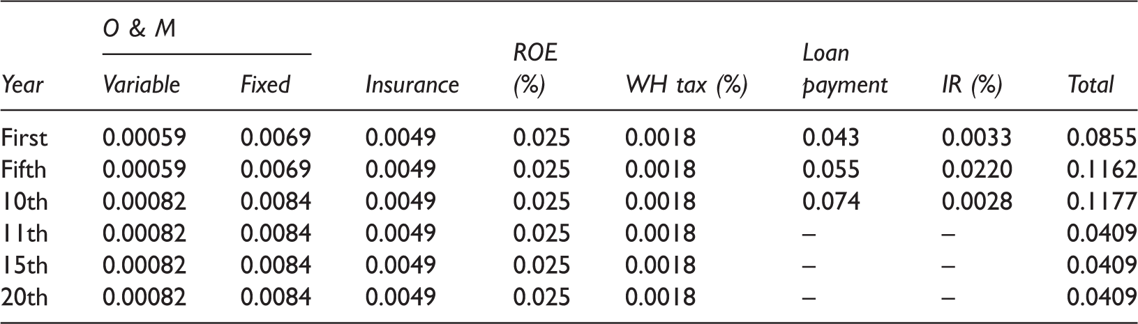
O & M: operation and maintenance; ROE: return on the equity; WH = with holding tax; IR: interest rate.

Note: All mentioned cost/kWh can be read as US$(cents)/kWh.

The economic analysis demonstrates the impact of energy lost and tariff economic model based on setting of annual energy output, OM costs, insurance and return of equity. As a major chunk of expenses of wind turbine is expended on installation and reducing the OM costs is one of important measure to reduce the total cost (Al-Najjar and Hailemariam, 2012). The net loan repayment and interest rate is within the bounds of what is required for the wind turbine to cover loan and interest within the time frame of 10 years. The calculations exhibit an average LCOE value US$(cents) 0.1137/kWh for the first 10 years (from 1 to 10 years). The LCOE will be decreased to US$(cents) 0.040/kWh for next 10 years (from 11 to 20 years). The average LCOE is US$(cents) 0.0802/kWh for period of 20 years. The difference between 1 to 10 years and 11 to 20 years is US$(cents) 0.0728/kWh. Figure 14 is showing the decreased LCOE for the life of 20 years of the wind farm. The economic model showed the effect of wind energy penetration on the price of electricity purchased by Water and Power Development Authority, Pakistan (WAPDA).

Figure 14.

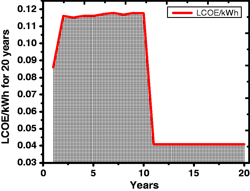
Levelized tariff and cost of energy (US$/kWh) for 20 years.

The wind farm performance showed the potential rise in the energy generation in first and second year of operation. The energy generation rose up 15.50 and 21.10% to set bench mark of 142 GWh energy in first and second year, respectively. If energy generation increased to set benchmark with the year passing would have significant effect on the levelized cost and tariff of energy. The results of LCOE model showed a significant drop in the cost per kWh. However, the only contributing factor is maximum real availability of wind turbine system.

Conclusions

In this paper, the assessment of local wind characteristics, performance, levelized tariff and cost of energy for a period of 20 years has been carried out for wind farm located at Jhimpir, Pakistan. An assessment of the local wind characteristics has been carried to find out an intensity of wind speed (m/s) presented over a period of a year. Weibull distribution is an important indicator for future wind conditions at the location. The mean Weibull k and c parameter and standard deviation were found to be 3.360 and 8.940 m/s and 2.563, respectively. The performance function of wind farm is investigated for a period of two years. The technical and real availability found to be 97 and 90%, respectively. The real availability decreased due to low wind, wind turbine component failure, grid and distribution loss. The capacity factor increased to 35.50% in second year compared to first year. The power coefficient is dropped if wind speed crosses the rated power. So it can be concluded that the efficiency of wind turbine is decreased due to increased wind speed (m/s). It is also concluded that the wind turbines works efficiently at the wind speed between 6 and 10 m/s. Tip speed ratio shows that the wind turbine operating close to optimal lift and drag will exhibit the performance level. The proposed levelized tariff and cost of energy model based on set energy generation benchmark of 142 GW showed a significant influence on the energy cost per kWh. The cost per kWh is US$(Cents) 0.11371 and 0.04092 for 1–10 and 11– 20 years, respectively. The energy output showed a significant impact on LCOE if it produced beyond the 142 GWh per year. In this regard, the different scenarios are studied which showed a positive effect on the LCOE for 20 years. The renewable energy has tremendous impact on LCOE as compared to non-renewable source of energy.

Footnotes

Declaration of conflicting interests

The author(s) declared no potential conflicts of interest with respect to the research, authorship and/or publication of this article.

Funding

The author(s) received no financial support for the research, authorship and/or publication of this article.

References

Akpinar

(2005) An assessment on seasonal analysis of wind energy characteristics and wind turbine characteristics. Energy Conversion and Management 46: 1848–1867.

Al-Najjar

Hailemariam

(2012) Maintenance solutions for continuous & cost-effective improvement of wind turbine performance. IFAC Proceedings Volumes 45: 151–156.

Amar

Elamouri

Dhifaoui

(2008) Energy assessment of the first wind farm section of Sidi Daoud, Tunisia. Renewable Energy 33: 2311–2321.

Ammara

Leclerc

Masson

(2002) A viscous three-dimensional differential/actuator-disk method for the aerodynamic analysis of wind farms. Journal of Solar Energy Engineering 124: 345–356.

Asif

(2009) Sustainable energy options for Pakistan. Renewable and Sustainable Energy Reviews 13: 903–909.

Bezrukovs

Zacepins

Bezrukovs

et al . (2016) Comparison of methods for evaluation of wind turbine power production by the results of wind shear measurements on the Baltic shore of Latvia. Renewable Energy 96: 765–774.

Bhatt

Jothibasu

(2002) Prediction and enhancement of performance of wind farms in India. Journal of Scientific and Industrial Research 61: 1056–1062.

Blanco

(2009) The economics of wind energy. Renewable and Sustainable Energy Reviews 13: 1372–1382.

Boubault

Hall

et al . (2016) Levelized cost of energy (LCOE) metric to characterize solar absorber coatings for the CSP industry. Renewable Energy 85: 472–483.

10.

Carroll

McDonald

McMillan

(2015) Failure rate, repair time and unscheduled O&M cost analysis of offshore wind turbines. Wind Energy 19(6): 1107–1119.

11.

Cooney

Byrne

Lyons

et al . (2017) Performance characterisation of a commercial-scale wind turbine operating in an urban environment, using real data. Energy for Sustainable Development 36: 44–54.

12.

Dokopoulos

Saramourtsis

Bakirtzis

(1996) Prediction and evaluation of the performance of wind-diesel energy systems. IEEE Transactions on Energy Conversion 11: 385–393.

13.

Eberhard

Kåberger

(2016) Renewable energy auctions in South Africa outshine feed‐in tariffs. Energy Science & Engineering 4: 190–193.

14.

Faulstich

Lyding

Tavner

(2011) Effects of wind speed on wind turbine availability. Proceedings of the 2011 European Wind Energy Conference.

15.

Ganjefar

Mohammadi

(2016) Variable speed wind turbines with maximum power extraction using singular perturbation theory. Energy 106: 510–519.

16.

Gao

Yang

(2016) Optimization of wind turbine layout position in a wind farm using a newly-developed two-dimensional wake model. Applied Energy 174: 192–200.

17.

Gurgur

Jones

(2010) Capacity factor prediction and planning in the wind power generation industry. Renewable Energy 35: 2761–2766.

18.

Hemmati

(2017) Technical and economic analysis of home energy management system incorporating small-scale wind turbine and battery energy storage system. Journal of Cleaner Production 159: 106–118.

19.

Herbert

Iniyan

Goic

(2010) Performance, reliability and failure analysis of wind farm in a developing country. Renewable Energy 35: 2739–2751.

20.

Igba

Alemzadeh

Henningsen

et al . (2015) Effect of preventive maintenance intervals on reliability and maintenance costs of wind turbine gearboxes. Wind Energy 18: 2013–2024.

21.

Kanyako

Janajreh

(2015) Implementation and economical study of HAWT under different wind scenarios. Sustainable Cities and Society 15: 153–160.

22.

Keyhani

Ghasemi-Varnamkhasti

Khanali

et al . (2010) An assessment of wind energy potential as a power generation source in the capital of Iran, Tehran. Energy 35: 188–201.

23.

Lai

Lin

(2006) Technical assessment of the use of a small-scale wind power system to meet the demand for electricity in a land aquafarm in Taiwan. Renewable Energy 31: 877–892.

24.

Andrews

(2015) Modelling wind turbine degradation and maintenance. Wind Energy 19(4): 571–591.

25.

Marvuglia

Messineo

(2012) Monitoring of wind farms’ power curves using machine learning techniques. Applied Energy 98: 574–583.

26.

Mejía

Chejne

Smith

et al . (2006) Simulation of wind energy output at Guajira, Colombia. Renewable Energy 31: 383–399.

27.

Meneguzzo

Ciriminna

Albanese

et al . (2016) The remarkable impact of renewable energy generation in Sicily onto electricity price formation in Italy. Energy Science & Engineering 4: 194–204.

28.

Millward-Hopkins

Tomlin

et al . (2013) Assessing the potential of urban wind energy in a major UK city using an analytical model. Renewable Energy 60: 701–710.

29.

Nejad

Gao

Moan

(2014) On long-term fatigue damage and reliability analysis of gears under wind loads in offshore wind turbine drivetrains. International Journal of Fatigue 61: 116–128.

30.

Neuteleers

Mulder

Hindriks

(2017) Assessing fairness of dynamic grid tariffs. Energy Policy 108: 111–120.

31.

Nilsson

Bertling

(2007) Maintenance management of wind power systems using condition monitoring systems—life cycle cost analysis for two case studies. IEEE Transactions on Energy Conversion 22: 223–229.

32.

O’Dell

(2001) Improved blade designs and manufacturing processes reduce the cost of wind energy. Journal of Solar Energy Engineering 123: 268–268.

33.

O’Flaherty

Riordan

O’neill

et al . (2014) A quantitative analysis of the impact of wind energy penetration on electricity prices in Ireland. Energy Procedia 58: 103–110.

34.

Parrado

Girard

Simon

et al . (2016) 2050 LCOE (levelized cost of energy) projection for a hybrid PV (photovoltaic)-CSP (concentrated solar power) plant in the Atacama Desert, Chile. Energy 94: 422–430.

35.

Pelletier

Masson

Tahan

(2016) Wind turbine power curve modelling using artificial neural network. Renewable Energy 89: 207–214.

36.

Petković

Ćojbašič

Nikolić

(2013) Adaptive neuro-fuzzy approach for wind turbine power coefficient estimation. Renewable and Sustainable Energy Reviews 28: 191–195.

37.

Puglia

Bangalore

Tjernberg

(2014) Cost efficient maintenance strategies for wind power systems using LCC. In: Probabilistic methods applied to power systems (PMAPS) 2014 international conference on IEEE, pp.1–6.

38.

Ribrant

Bertling

(2007) Survey of failures in wind power systems with focus on Swedish wind power plants during 1997-2005. In: Power engineering society general meeting 2007 IEEE. IEEE, pp.1–8.

39.

Schlechtingen

Santos

Achiche

(2013) Using data-mining approaches for wind turbine power curve monitoring: A comparative study. IEEE Transactions on Sustainable Energy 4: 671–679.

40.

Şen

(1997) Statistical investigation of wind energy reliability and its application. Renewable Energy 10: 71–79.

41.

Shahizare

Nik-Ghazali

Chong

et al . (2016) Novel investigation of the different Omni-direction-guide-vane angles effects on the urban vertical axis wind turbine output power via three-dimensional numerical simulation. Energy Conversion and Management 117: 206–217.

42.

Shami

Ahmad

Zafar

et al . (2016) Evaluating wind energy potential in Pakistan's three provinces, with proposal for integration into national power grid. Renewable and Sustainable Energy Reviews 53: 408–421.

43.

Sheikh

(2010) Energy and renewable energy scenario of Pakistan. Renewable and Sustainable Energy Reviews 14: 354–363.

44.

Shu

Chan

(2015) Statistical analysis of wind characteristics and wind energy potential in Hong Kong. Energy Conversion and Management 101: 644–657.

45.

Sørensen

Unnikrishnan

Mathew

(2001) Wind farms connected to weak grids in India. Wind Energy 4: 137–149.

46.

Starke

Cardemil

Escobar

et al . (2016) Assessing the performance of hybrid CSP+ PV plants in northern Chile. Solar Energy 138: 88–97.

47.

Toft

Svenningsen

Moser

et al . (2016) Wind climate parameters for wind turbine fatigue load assessment. Journal of Solar Energy Engineering 138: 031010.

48.

Ucar

Balo

(2009) Evaluation of wind energy potential and electricity generation at six locations in Turkey. Applied Energy 86: 1864–1872.

49.

Veers

Winterstein

(1998) Application of measured loads to wind turbine fatigue and reliability analysis. Journal of Solar Energy Engineering 120: 233–239.

50.

Wang

Huang

et al . (2016) Wind turbines abnormality detection through analysis of wind farm power curves. Measurement 93: 178–188.

51.

Wang

Teah

(2017) Life cycle assessment of small-scale horizontal axis wind turbines in Taiwan. Journal of Cleaner Production 141: 492–501.

52.

Yang

Wen

et al . (2016) Estimation of wind power generation in dense urban area. Applied Energy 171: 213–230.

53.

Yang

Burnett

(2003) Weather data and probability analysis of hybrid photovoltaic–wind power generation systems in Hong Kong. Renewable Energy 28: 1813–1824.

54.

Yearbook

(2016) Hydrocarbon development institute of Pakistan. Ministry of Petroleum and Natural Resources, Government of Pakistan.

55.

Zhao

Chen

Thomson

(2017) Levelized cost of energy modeling for concentrated solar power projects: A China study. Energy 120: 117–127.

Assessment of the apparent performance characterization along with levelized cost of energy of wind power plants considering real data

Abstract

Keywords

Introduction

Site description and local wind data measurement

Methodology

Wind characteristics and Weibull distribution functions

Wind farm performance analysis model

Capacity factor

Power curve analysis

Power coefficient

Tip speed ratio

Availability factor analysis

LCOE model

Results and discussion

Wind characteristics of site

Wind speed

Wind direction

Weibull distribution function

Frequency distribution of wind

Performance analysis model

Power curve analysis

Power coefficient

Tip speed ratio

Availability factor analysis

Measured data

Capacity factors

LCOE model

Conclusions

Footnotes

Declaration of conflicting interests

Funding

References