Sage Journals: Discover world-class research

Abstract

Previous research has established that low-wage earners have on average lower job satisfaction. However, several studies have found personal characteristics, such as gender, age and educational level, moderate this negative impact. This article demonstrates additional factors at the household level, which have not yet been empirically investigated, and which may exacerbate gender differences. The authors analyse the job satisfaction of low-wage earners depending on the contribution of individual earnings to the household income and on household deprivation using the 2013 special wave of the EU-SILC for 18 European countries. The study finds that single earners in low-wage employment report lower job satisfaction whereas low-wage employment does not seem to make a difference for secondary earners. Furthermore, low-wage earners’ job satisfaction is linked with the ability of their household to make ends meet.

Keywords

Earner position household context job satisfaction low wage poverty

Introduction

Low-wage employment is a growing segment of most labour markets in the European Union (EU Commission, 2017). In 2014, 17.2% of all employees in the 28 EU member states received a wage below two-thirds of the national median wage (Eurostat, 2016). Additionally, in-work poverty is rising and full- or near full-time work does not necessarily safeguard against poverty (Andreß and Lohmann, 2008; Cooke and Lawton, 2008; García-Pérez et al., 2016; Giesselmann and Lohmann, 2008; Lohmann and Marx, 2018; Marchal and Marx, 2017; Ponthieux, 2010). This vein of research focused on the composition of low-wage workers and in-work poverty; other aspects, such as job satisfaction of low-wage workers, have hardly received any attention.

In contrast, job satisfaction research has dealt superficially with low-wage earners. Generally, low-wage earners are reported to have a lower level of job satisfaction than their higher-paid counterparts (Diaz-Serrano and Cabral, 2005). However, Sloane and Williams (2000) report for the UK that low-wage workers show higher levels of job satisfaction in contrast to higher-wage workers.¹ They partially attribute this finding to composition effects, i.e. to the fact that the low-paid are overwhelmingly young, female and less educated (see also Lucifora and Salverda, 2009: 266). As Clark (1998) rightfully posits, income is just one factor that influences workers’ job satisfaction. It is possible that low-paid jobs might provide compensating differentials in the form of non-pecuniary benefits (Leontaridi and Sloane, 2001), but the low quality of many low-wage jobs (McClelland and Holman, 2015) and the combination of low wage with atypical forms of employment (Olsthoorn, 2014) raise doubts about the quantity of these non-pecuniary benefits. Moreover, the effect of low wages on job satisfaction is likely exacerbated when the remuneration is unrelated to the actual demands and efforts of the work (regarding effort–reward imbalances, see Siegrist, 2010, 2012).

These diverging results on the job satisfaction of low-wage workers may be influenced by the gendered distribution and valuation of work and tasks in the household. Navarro and Salverda (2019) have recently shown that a person’s contribution to the household income affects job satisfaction. While quantitative studies have not yet explored this topic for low-wage workers, the qualitative study by Sardadvar et al. (2017) identified several buffering effects related to the household context that make low income acceptable, inter alia the pooling of resources within a household can create a ‘together we get by’ pattern. In this article, we explore this effect from pooled resources and intra-household relations on job satisfaction. Our overarching research question is whether household context matters for low-wage earners’ job satisfaction. We focus on two possibly involved factors. First, the earner’s contribution to the household income is studied as a proxy for the role of the earner in the household and the necessity of the wage, as low-wage jobs are often chosen as additional income. Second, we study whether low-wage earners living in a poor household demonstrate the so-called ‘together we get by’ pattern.

To investigate these relationships, we employ regression analysis using the 2013 special wave from the European Union Statistics on Income and Living Conditions (EU-SILC) survey focusing on life satisfaction. The earners’ position in the household is taken into consideration, distinguishing between single earners, main earners, dual main earners as well as secondary earners. By portraying the specific case of low-income earners in determinants of job satisfaction, we extend both employment-related aspects and household factors.

Job satisfaction: Work and non-work-related factors of explanation

Job satisfaction is an overall attitude people have towards their job (Kalleberg, 1977). Economists use job satisfaction in particular to provide a single metric of a current job compared with alternative opportunities (Hamermesh, 2001). The exact definition of job satisfaction and the acknowledged determinants of job satisfaction vary as to whether a situational or dispositional perspective is adopted (Fernández-Macias and Muñoz de Bustillo Llorente, 2014; Judge and Klinger, 2008). The situational perspective emphasizes the objective assessment of job characteristics for job satisfaction. The most important characteristics are firstly related to the work contract, such as salary, contract type (fixed-term/open), job security and working hours, and secondly the job content, such as the ability to take decisions, the variation of job tasks, the career and training opportunities, and the support provided by colleagues (Judge and Klinger, 2008; Warr, 2007). Additionally, more distant factors such as commuting time, business-related travel and social status associated to the profession are important (cf. Coppin and Vandenbrande, 2007). Thus, the situational perspective proposes that low wages will lead to decreasing job satisfaction if there are no compensating differential benefits.

In line with the situational perspective, many studies confirm that job satisfaction is related to the comparative wage level (Card et al., 2012; Clark and Oswald, 1996). In most European countries, low-paid workers report a lower level of job satisfaction than higher-paid workers (Diaz-Serrano and Cabral, 2005). Interestingly, it also has been shown that the job satisfaction of low-wage workers is particularly sensitive to comparative information about their low pay within a company (Card et al., 2012). Other case studies have found that low-paid jobs might provide compensating differentials in the form of non-pecuniary benefits (Leontaridi and Sloane, 2001). In line with the situational approach we expect that the relative wage level has a strong effect on job satisfaction and that satisfaction will be lower among low-wage workers. Other employment characteristics related to precariousness such as fixed-term contracts or part-time employment may also be important, but we expect that they will be less connected to the financial dimension of job satisfaction.

In contrast, the dispositional perspective argues that job satisfaction is co-determined by a person’s traits, expectations, values and needs (Judge and Klinger, 2008; Kalleberg, 1977; Kalleberg and Mastekaasa, 2001). Thus, personal characteristics and contextual factors may alleviate or exacerbate negative effects of low wages on job satisfaction. In the literature, various personality concepts (Judge and Klinger, 2008), work values (Kalleberg, 1977; Zou, 2015) and many socio-demographic proxies, such as age (Clark et al., 1996; Mottaz, 1987), gender (Clark, 1997; Zou, 2015), race/ethnicity (Verkuyten et al., 1993), occupation and social class (Kalleberg and Griffin, 1978), have been studied as dispositional factors.

Regarding low-wage workers, Sardadvar et al. (2017) found four dispositional aspects that can buffer job satisfaction despite the low financial compensation: a ‘better than nothing’ pattern (lack of alternatives due to low education, skills recognition or stereotypes), a prior bad work experience, a comparison of their current level of income to the level they would have in their country of origin, and a ‘together we get by’ pattern (low wages may be compensated by other household members’ income). This implies that low remuneration may not be associated with a lower satisfaction if pooling and sharing of resources within a household provide workers with enough resources. Hence, ‘a wage that somebody is satisfied with is not necessarily a living wage’ (Sardadvar et al., 2017: para. 38). The ‘together we get by’ pattern stresses the point that although a person’s wage is an important element of the disposable household income, living conditions and deprivation are determined by the pooled income of all household members in relation to the household’s composition and needs.

For our research question, both perspectives may be considered complementary rather than contradictory. For example, gender has been found to be an important factor of job satisfaction (Bender et al., 2005; Clark, 1997; Rigotti et al., 2015; Zou, 2015). These gender differences can be partially attributed to situational job characteristics due to the gendered division of labour: in Western Europe, women are more likely to work part-time or to do unpaid housework and care work. Low pay is also more prevalent among women, most likely to work in the service sector (Bosch, 2009; Brülle et al., 2019). Additionally, there are still large gender differences in occupations, economic sectors and contract type. ‘Gender contracts’ reflecting households’ arrangements in balancing paid work and care work are not simply a result of individual preferences. The outcome of the partners’ negotiations is a combination of practices, norms, values, structural factors and institutional opportunities (Aboim, 2010; Dingeldey, 2016; Lomazzi et al., 2018; Pfau-Effinger, 2005). Nonetheless, the worse situational job characteristics of women do not necessarily lead to lower job satisfaction. Instead, dispositional factors such as expectations and values may determine a household’s distribution of work and the assessment of jobs. Therefore, we argue that research should explicitly take into account the household and the work–family nexus as it could be a possible moderator of the expectations towards and the assessment of a low-wage job. Rigotti et al. (2015) emphasize that the social position and the motives underlying a job will modify the relation between job characteristics and job satisfaction. Navarro and Salverda (2019) have found that job satisfaction is highest among men who are the sole earner or main earner in a couple. Equal contributions or even lower contributions to a couple’s earnings lead to less job satisfaction. In contrast, women only show lower job satisfaction if they are the secondary earners. Based on this finding, we assume that the job satisfaction of a low-wage earner varies according to the dependency of the household on his or her earnings. Higher financial expectations contribute to lower job satisfaction when they are harder to meet in the case of low-wage jobs. Single earners or main earners are more likely to face expectations for higher income. Particularly, single-parent households, where the parent often works part-time (e.g. due to inadequate childcare provision), may face very high financial requirements which are unattainable with low-wage employment.² Similarly, we assume that the negative effects of low-wage employment may be mitigated for additional earners in so-called ‘secondary jobs’. In dual earner households, financial requirements and risks can be shared with a second person whose income is approximately as high as the income of the first person, possibly reducing the detrimental effect of low-wage employment.

H1: The difference in job satisfaction between persons who either earn a low wage or earn above the low wage level is larger for single earners or main earners compared to secondary or dual main earners.

Pooling of resources within a household may lift a household out of poverty. Consequently, low-wage employment does not lead to poverty as long as other household members contribute to the household income (Dingeldey and Berninger, 2013; Maître et al., 2012). This finding is supported by evidence that between the years 2005 and 2014 individual poverty was reduced by around 22% by pooling labour earnings within households within the EU (Eurofound, 2017). Thus, the household composition determines the likelihood of a low-paid worker to be poor, next to labour market characteristics and social as well as tax policies (Andreß and Lohmann, 2008; Crettaz and Bonoli, 2011). If low wages are balanced out by other income sources within a household, or if non-financial motives for a job prevail, job satisfaction is possibly unaffected by low wages. In these cases, the social integration stemming from the job and a possibly higher work–life balance of low-paid jobs may increase job satisfaction. However, we expect a negative impact on job satisfaction for low-wage workers living in poor households (i.e. ‘still not enough’ effect).

H2: A household income below the poverty threshold exacerbates the negative impact of a low wage on a worker’s job satisfaction.

Hence, we envision job satisfaction of low-wage workers as influenced by the financial contribution a worker makes to the household income and by household poverty as we assume that the financial dimension of a job becomes more important if the individual contribution to the household budget is larger or if the household is experiencing financial stress.

Data and method

The article analyses job satisfaction employing the EU-SILC user database from 2013, which included a special survey module on well-being, such as job satisfaction and life satisfaction (cf. for an introduction into the EU-SILC, Atkinson et al., 2017). The EU-SILC has been collecting cross-sectional and longitudinal information on living conditions and income from the EU member states and associated partners since 2004. The EU-SILC combines nationally representative samples of households. It is ex-ante output-harmonized, meaning that it is based on a common framework but leaves leeway to the member states in deciding on their sampling and data collection methods (Goedemé, 2013; Iacovou et al., 2012). We pool data from the user database from April 2019 for 18 countries consisting of the EU-15 and the three EFTA countries, namely from Austria, Belgium, Denmark, Finland, France, Germany, Greece, Italy, Ireland, Luxembourg, Netherlands, Portugal, Sweden, Spain, United Kingdom, Norway, Switzerland and Iceland. This allows us to generalize statements to most Western European countries.

We decided to restrict our sample to Western European countries, in order to limit the divergence of income inequality and purchasing power between countries (cf. Goedemé, 2019). Moreover, practices of paying ‘envelope wages’ are more common in Eastern European countries (Williams, 2008). As our main aim is to assess the individual in respect to the household level, we adjusted for country-level differences using country dummies in the regression analysis.³ For robust estimates, we calculated hourly wages restricting our sample to full-year workers (cf. Maître et al., 2012). Those workers who were not employed during 12 months of the year had to be excluded to facilitate the calculation of the hourly wages, which are based on information of the yearly income.⁴ Consequently, our results are conservative because we exclude unstable employment trajectories. We also restricted the sample to persons aged 25–55 and those in dependent employment relations. Self-employed persons were excluded as they have other job rewards (such as high work autonomy) and as their work income may follow different logics than the wage of dependent employees. For the same reason, individuals during training and education periods and pre-retirement were excluded from the analysis. We distinguished between workers holding a full-time or a part-time contract. For the 18 countries in the study, the sample size is 54,025 working people.

Job satisfaction refers to the respondent’s attitude about the degree of satisfaction with his or her job. It is measured using an 11-point scale from 0 (‘not at all satisfied’) to 10 (‘completely satisfied’). It reflects a snapshot of the current appraisal of all job areas. Low-wage is defined as a gross hourly wage below two-thirds of the national median gross hourly wage (Diaz-Serrano and Cabral, 2005; Lucifora and Salverda, 2009). We employed a threshold of 60% of the national equivalized median income as an indicator for household poverty (Atkinson et al., 2002). The household income is calculated from the total disposable income (gross household income minus taxes, compulsory social insurance contributions and inter-household transfers paid) weighted with the OECD household equivalence scale.

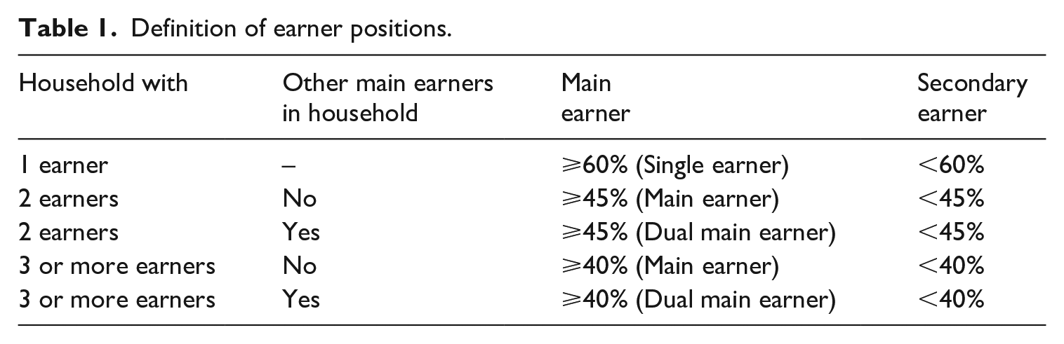
To distinguish the influence of different household settings, we created a variable defining each individual’s contribution to the household income compared to the contributions of other household members. The typology of earnings’ contributions by Raley et al. (2006), which compares the share of joint earnings in couples, has been frequently used in the literature. A problem with this typology and similar approaches is that it only focuses on wages and overlooks income from self-employment, pensions, or other personal social benefits such as unemployment or sickness. However, benefits may be an important source of income for low-wage earners’ households. Moreover, households with more than two employed persons are in most cases excluded. As our data contain no information about the intra-household distribution of direct transfers to households, we focused on personal income sources which observably influence the share of contributions to a household’s income. In the first step, we summed up all personal income sources (from wages, self-employment earnings, pensions, unemployment benefits, old age benefits, sickness benefits, disability benefits and educational allowances/benefits) from all household members (including persons aged below 25 and above 56 as well as self-employed and retirees). In the next step, we calculated the ratio between a person’s gross earnings from dependent work (and from possible other second jobs in self-employment) and a household’s total personal income. Based on this ratio, we differentiated between secondary earners and different types of main earners using the following thresholds.⁵ As shown in Table 1, we defined a single earner as living in a household without other wage earners and whose gross earnings contribute 60% or more of the household income. To capture only substantive contributions to the household income, we defined all workers as main earners whose earnings amount to 45% or more in a household with two wage earners and 40% or more in households with three or more wage earners. As the contributed share of the household income depends on the number of earners in the household (cf. Figure A1 in the Appendix), we set the threshold in two-earner households slightly higher than for households with three earners or more. In the case of households with two main earners, we labelled both as dual main earners. Although this reflects a rather limited definition of dual main earner households, it helps to distinguish when the burden of income generation is rather equally shared. All persons whose wage contributions fell below these thresholds were classified as secondary earners. As an effect, there could be households without a main earner, as the income from work did not contribute the main share of household income attributable to household members.

Table 1.

Definition of earner positions.

Household with	Other main earners in household	Main earner	Secondary earner
1 earner	–	⩾60% (Single earner)	<60%
2 earners	No	⩾45% (Main earner)	<45%
2 earners	Yes	⩾45% (Dual main earner)	<45%
3 or more earners	No	⩾40% (Main earner)	<40%
3 or more earners	Yes	⩾40% (Dual main earner)	<40%

Based on these operationalizations, we apply a linear regression model with robust standard errors clustered within households to account for household dependencies. For all descriptive statistics, cross-sectional personal weights are used. Additionally, several individual covariates adjust for the effects of gender, migrant status, age, education and subjective health on job satisfaction in the regression models. To reflect job-related effects of wage income, part-time employment, temporary employment (fixed-term contract), occupation and supervisory position and economic sector were included in the model. Moreover, we distinguished various household types: singles, two adults (or more) without children, single-parent households and households with at least two adults and children.

Results

Sample characteristics

Table 2 shows demographic characteristics for the sample of 25- to 55-year-old employed persons in the 18 countries. The first and second column show the characteristics of the persons from the sub-samples of 12 months full-time employed and 12 months part-time employed persons, who were analysed in the regression analysis. We see a clear gendered pattern as approximately 60% of full-time workers are men and almost 90% of part-time workers are women. At 42%, the share of persons who finished tertiary education is much higher in full-time than in part-time work. Full-time employees also consider themselves healthier than part-time employees, pointing to a potential self-selection into part-time work. This could also be because part-time workers are slightly older.

Table 2.

Demographic and household characteristics of sample.

	Full-time employedfor 12 mo.	Part-time employedfor 12 mo.	Less than12 mo. employed	Total
Gender (Col. %)
Male	59.6	11.6	44.3	49.5
Female	40.4	88.4	55.7	50.5
Age
Mean	41.1	42.4	39.0	41.0
SD	8.5	8.1	8.7	8.5
Migrant status (Col. %)
Native	87.9	85.9	83.2	86.9
Migrant	12.1	14.1	16.8	13.1
Education (Col. %)
Lower secondary and below	13.1	15.9	17.9	14.3
Upper secondary	45.3	55.9	41.7	46.5
Tertiary education	41.6	28.2	40.4	39.2
Self-rated health (Col. %)
Very good or good	84.3	79.4	81.7	83.1
Fair	13.8	17.4	16.0	14.7
Bad or very bad	1.9	3.3	2.3	2.2
Hourly wage (Col. %)
Above low-wage level	91.2	72.5		87.6
Below low-wage level	8.8	27.5		12.4
Household type (Col. %)
One-person household	20.3	8.7	18.6	18.1
Adults, no children	32.6	25.4	29.6	30.9
Single-parent household	3.8	8.5	5.5	4.8
Adults with children	43.4	57.3	46.3	46.1
Earner position (Col. %)
Secondary earner	21.7	68.6	49.7	33.5
Single earner	36.1	19.1	29.2	32.3
Main earner	28.7	6.3	14.8	23.0
Dual main earner	13.4	6.0	6.2	11.2
Household income (Col. %)
Above poverty line	96.0	87.7	84.2	92.9
Below poverty line	4.0	12.3	15.8	7.1
Job satisfaction (0 = not at all, 10 = very satisfied)
Mean	7.2	7	7	7.1
SD	1.9	2.1	2.2	2
N	45,584	10,586	10,902	67,072

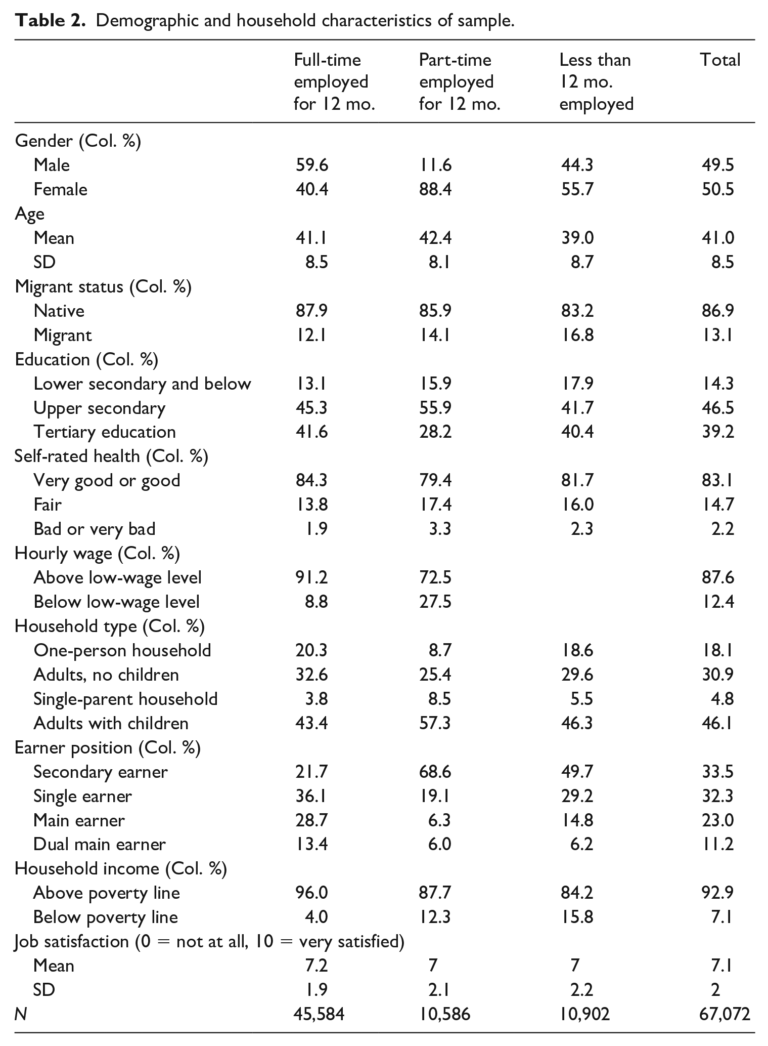
As to be expected, among the full-time workers, single and main earners were the majority while most part-time workers were secondary earners. Dual main earners are still relatively rare but more frequent on a full-time than on a part-time basis. The part-time group has noticeably higher shares of single-parent households and of households with two or more adults with children. The share of persons who earn a low hourly wage is also substantially higher in the part-time group. Consequently, the share of persons who live in households whose equivalized, disposable income is below the poverty threshold is almost three times as high among the part-time employed than among the full-time employed.

Descriptive results

To get a first overview of possible differences in job satisfaction, Figure 1 shows the distribution of job satisfaction among employees with wages above and below the low-wage threshold. The distribution is skewed to the left with a mode of 8 at the 11-point scale ranging from 0 to 10. As in previous studies, there were more low-wage workers with low to medium job satisfaction in comparison with workers with higher earnings. Interestingly, however, we also found that more low-wage workers claim the highest value for job satisfaction.⁶

Figure 1.

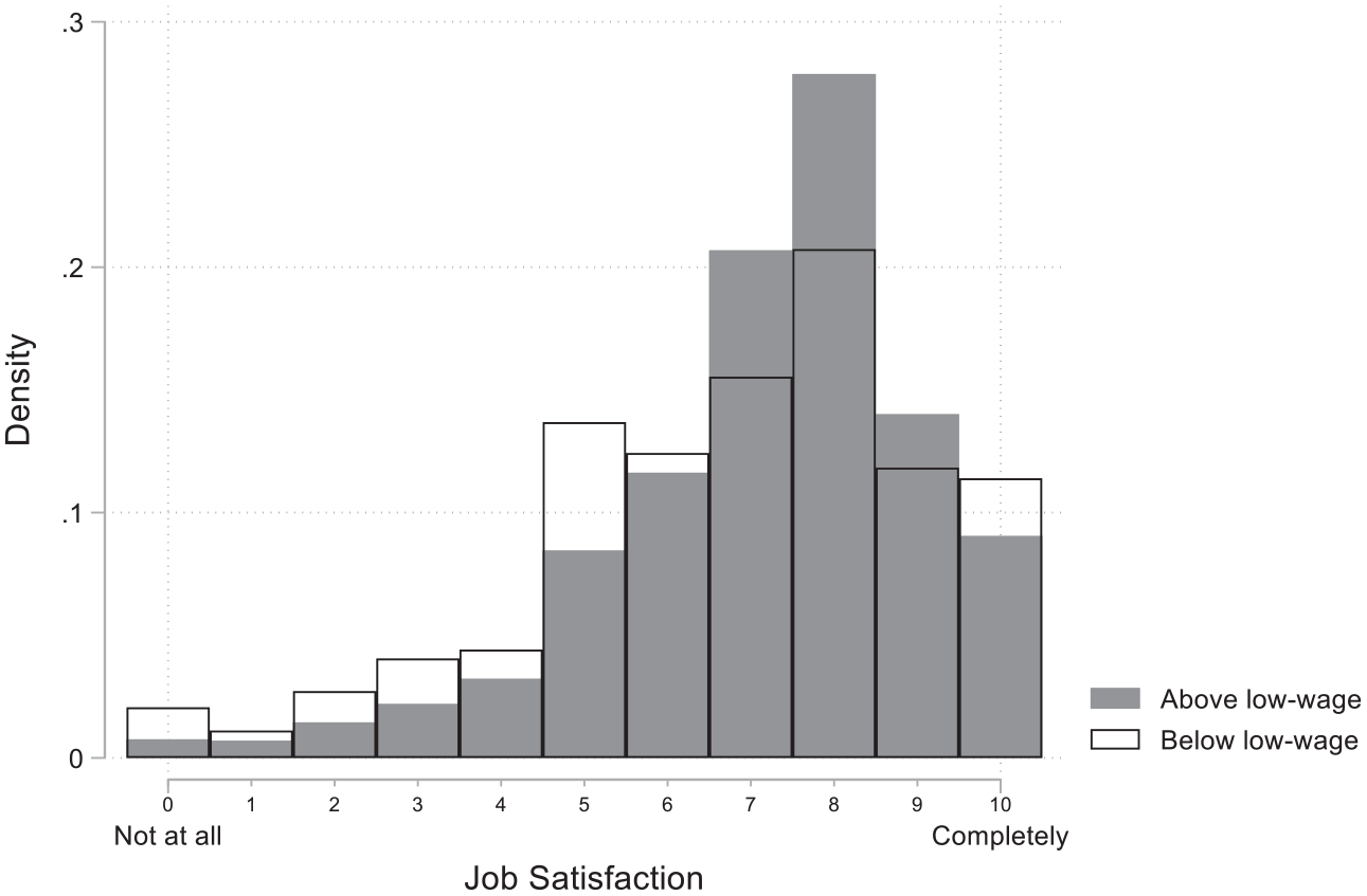
Distribution of job satisfaction among employees with wages above and below low-wage threshold.

Figure 2 compares the distribution of job satisfaction between earner positions. The job satisfaction of secondary earners was slightly more dispersed in medium values compared to the other earner positions. Low-wage earners reported lower satisfaction more frequently, despite the reported density in the highest satisfaction category. In contrast, among single earners, there are almost as many highly satisfied low-wage earners as among higher-wage earners. Low-wage earners who are single earners also report lower and especially medium job satisfaction more frequently than their counterparts with higher earnings. The panels for the main earner and dual main earner position show that low-wage earners from both types have much higher frequencies at both margins of the distribution. Thus, they report low and very high job satisfaction more often than higher-wage earners. Overall, Figure 2 indicates some differences between earner positions in line with Hypothesis 1 as job satisfaction of secondary earners is more evenly distributed for low-wage as well as higher-wage earners compared to the other earner positions.

Figure 2.

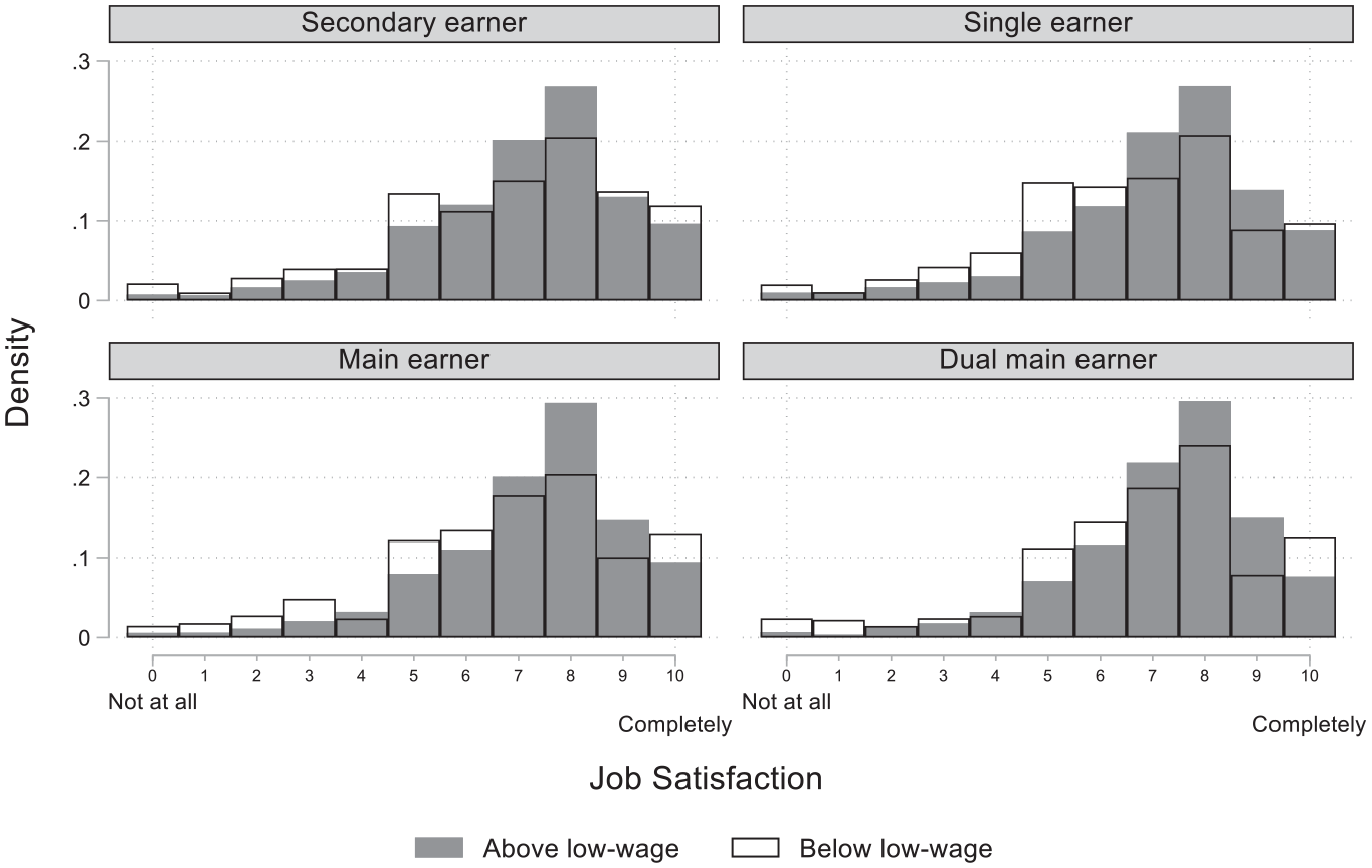
Distribution of job satisfaction among employees with different earner positions.

In Figure 3, we can see that among poor households, the distribution of job satisfaction is flatter and more skewed to the left so that the difference between low-wage earners and higher-wage earners is smaller. Although the mode lies again at 8, both distributions for low-wage and higher-wage earners in poor households show a rise at the highest job satisfaction. Overall, the group of low-wage earners in poor households who report high or the highest value for job satisfaction is smaller than the comparable group of higher-wage earners. The distribution of job satisfaction of low-wage workers in poor households is shifted towards smaller values of job satisfaction. This lends some descriptive support to Hypothesis 2 that low-wage employment has a stronger negative effect on job satisfaction if the household is poor.

Figure 3.

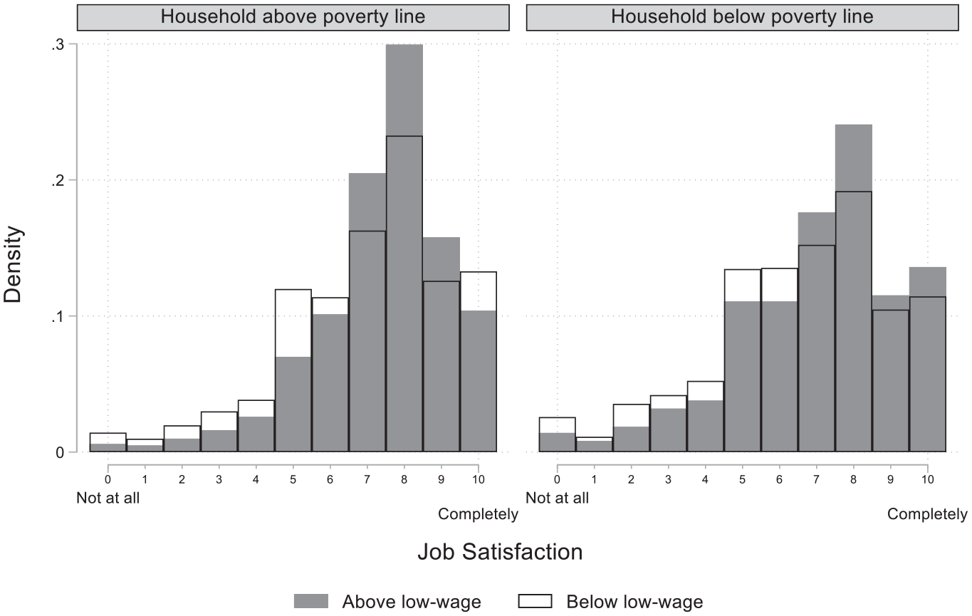
Distribution of job satisfaction among employees in poor/non-poor households.

Results from the regression analysis

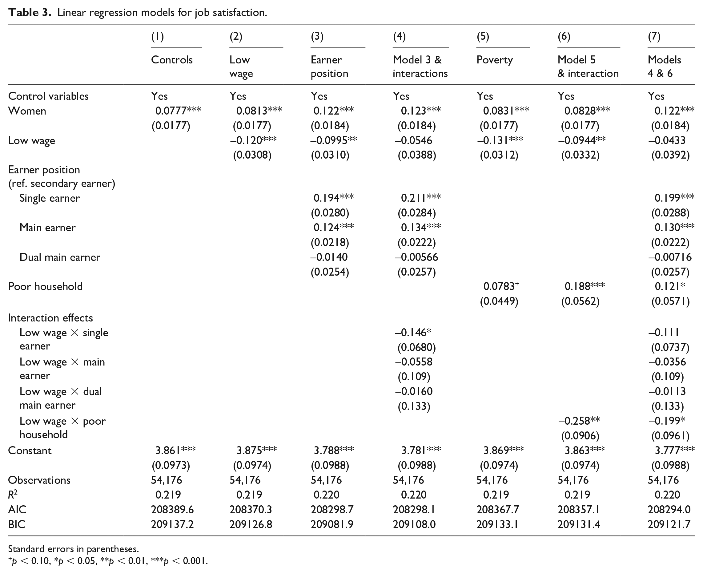
In Table 3, we present a series of regression models for job satisfaction. The models adjust for country and demographic variables (gender, migrant status and education), household types (singles, adults without children, single-parent households and adults with children), job-related variables (part-time employment, temporary contract, supervisory position, occupation, economic sector), self-rated health and life satisfaction (see Table A1 in the Appendix for the full results of the covariates).

Table 3.

Linear regression models for job satisfaction.

	(1)	(2)	(3)	(4)	(5)	(6)	(7)
	Controls	Low wage	Earner position	Model 3 & interactions	Poverty	Model 5& interaction	Models4 & 6
Control variables	Yes	Yes	Yes	Yes	Yes	Yes	Yes
Women	0.0777***	0.0813***	0.122***	0.123***	0.0831***	0.0828***	0.122***
	(0.0177)	(0.0177)	(0.0184)	(0.0184)	(0.0177)	(0.0177)	(0.0184)
Low wage		–0.120***	–0.0995**	–0.0546	–0.131***	–0.0944**	–0.0433
		(0.0308)	(0.0310)	(0.0388)	(0.0312)	(0.0332)	(0.0392)
Earner position(ref. secondary earner)
Single earner			0.194***	0.211***			0.199***
			(0.0280)	(0.0284)			(0.0288)
Main earner			0.124***	0.134***			0.130***
			(0.0218)	(0.0222)			(0.0222)
Dual main earner			–0.0140	–0.00566			–0.00716
			(0.0254)	(0.0257)			(0.0257)
Poor household					0.0783+	0.188***	0.121*
					(0.0449)	(0.0562)	(0.0571)
Interaction effects
Low wage × single earner				–0.146*			–0.111
Low wage × single earner				(0.0680)			(0.0737)
Low wage × main earner				–0.0558			–0.0356
Low wage × main earner				(0.109)			(0.109)
Low wage × dual main earner				–0.0160			–0.0113
Low wage × dual main earner				(0.133)			(0.133)
Low wage × poor household						–0.258**	–0.199*
Low wage × poor household						(0.0906)	(0.0961)
Constant	3.861***	3.875***	3.788***	3.781***	3.869***	3.863***	3.777***
	(0.0973)	(0.0974)	(0.0988)	(0.0988)	(0.0974)	(0.0974)	(0.0988)
Observations	54,176	54,176	54,176	54,176	54,176	54,176	54,176
R ²	0.219	0.219	0.220	0.220	0.219	0.219	0.220
AIC	208389.6	208370.3	208298.7	208298.1	208367.7	208357.1	208294.0
BIC	209137.2	209126.8	209081.9	209108.0	209133.1	209131.4	209121.7

Standard errors in parentheses.

p < 0.10, *p < 0.05, **p < 0.01, ***p < 0.001.

Model 1 is a reference model and contains only control variables. In accordance with previous studies, women showed slightly higher job satisfaction on average. Employees who are part-time employed or have a temporary contract had lower job satisfaction. Job satisfaction is graded by education as lower educated employees reported higher job satisfaction. Additionally, overall life satisfaction and general health had a strong impact, which supports the assumption that job satisfaction is also determined by subjective factors.

Model 2 adds a dummy variable for low-wage employment. The results confirm that low-wage earners are generally less satisfied with their employment than workers with higher wages.

Model 3 assesses the individual contribution to household income by using dummy variables for the earner position of the employees. The reference category consists of secondary earners whose wage income is not a main share of the total personal income in the household in contrast to the other three positions. Single earners and main earners showed higher job satisfaction. The effect for dual main earner was weak and insignificant. Thus, persons who contributed the main share to a household’s work-related income were on average more satisfied with their job than secondary earners. At the same time, the effect size of low-wage employment decreased in Model 3. This could indicate a composition effect, as many low-wage earners are secondary earners. Interestingly, the effect of being a woman has become considerably stronger compared to Model 1. Despite adjusting for gender differences contained in economic sector, occupation, contract type and part-time employment, it seems that the contribution to the household income acts as a suppressor for job satisfaction and that the gendered distribution of work and care in the household is damping the higher job satisfaction among women.

Model 4 employs interaction terms between low-wage employment and the three earner positions. The interaction between single earner and low-wage employment was significant and negative. The conditional main effect of low-wage employment was insignificant, which speaks of the high explanatory value of the earner positions.⁷ To show the overall effect, the conditional main effects and interactions from Model 4 are shown again as predicted means of job satisfaction in Figure 4. According to Figure 4, the mean job satisfaction would be slightly above 7.3 if all persons in the sample were single earners whose wage is below the low-wage threshold. If they earned more than the low-wage threshold, the job satisfaction would be slightly above 7.5. Hence, Figure 4 suggests that low-wage employment significantly decreases the job satisfaction of single earners. In contrast, secondary earners’ job satisfaction was not impaired: their predicted mean job satisfaction was approximately 7.25 regardless of earning a low or higher wage. Although the predicted means of main earners and dual main earners appear to illustrate that low-wage employment makes a small difference as well, the confidence intervals were too broad. Low-wage employment appeared to place significant pressure on single earners, while job satisfaction of secondary earners is rather stable despite being in a low-wage job. Hence, we find evidence to partially support Hypothesis 1 as job satisfaction of low-paid single earners was lower compared to higher-paid single earners, and secondary earners did not differ. However, we could not corroborate different effects for main earners or dual main earners. Surprisingly, low-paid dual main earners had the lowest predicted level of job satisfaction. As the group of low-wage dual main earners is still relatively small it is difficult to make inferences from the data.

Figure 4.

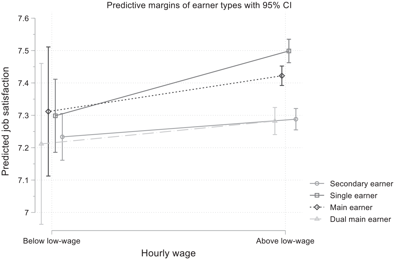
Adjusted predictions of mean job satisfaction for earner positions and low-wage employment based on Model 4.

Model 5 introduces a dummy variable for households whose equivalized, disposable income is below the poverty threshold of 60% of the national median household income. Surprisingly, household poverty seemed to slightly increase job satisfaction. In Model 6, we found a strongly negative interaction between low-wage employment and household poverty on job satisfaction. The conditional main effect of low-wage employment became weaker while the other conditional main effect of household poverty became stronger.⁸ For ease of interpretation, Figure 5 presents the predicted means of job satisfaction for household poverty and low-wage employment according to Model 6. Taken together, there was a significant, negative effect on job satisfaction, if all persons in the sample were low-wage earners living in poor households compared to higher-wage earners living in a poor household. For households above the poverty line, the predicted difference between low-wage and higher-wage earners is smaller. Thus, the results support Hypothesis 2 although there seems to be a motivational effect of living in poverty that is outweighed by the interaction with low-wage employment.

Figure 5.

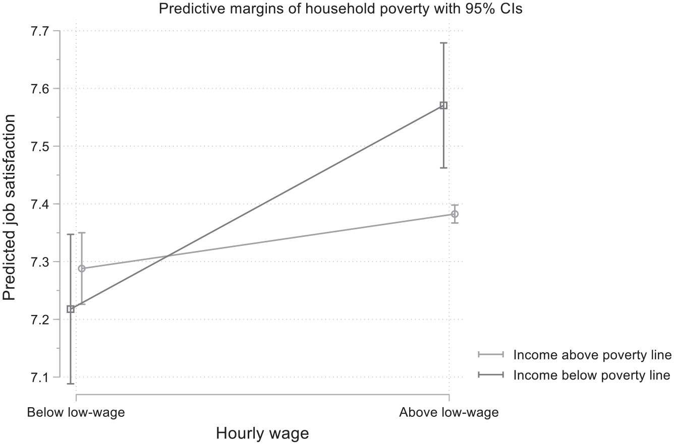
Adjusted predictions of mean job satisfaction for household poverty and low-wage employment based on Model 6.

Finally, Model 7 combines Models 4 and 6. This makes it possible to control for aggregate effects since single earners who earn a low wage are more likely to live in a poor household. The conditional main effects of the earner positions were very similar to the effects in Model 4, however, the effect for household poverty became weaker. The interaction effects for single earners in low-wage employment were weaker and became insignificant, possibly due to overlap between low-wage single earner households and poor households. Nonetheless, the adjusted predictions of mean job satisfaction in Figure 6 clearly depict how low-wage employment makes a difference for single earners who live in poor households. As can be seen in the figure, the model predicts no other significant differences.

Figure 6.

Adjusted predictions of mean job satisfaction for earner positions, household poverty and low-wage employment based on Model 7.

Discussion and conclusion

In this article, we used 2013 EU-SILC data to analyse the effects of a low-wage earner’s household context on job satisfaction. In our models, we introduced interaction terms between on the one hand low-wage employment, and on the other hand household poverty and earner positions, that allowed for more nuanced understanding of job satisfaction in specific household contexts. Our findings show that the household context is an important factor for job satisfaction that has scarcely been considered in research on job satisfaction. Taking into consideration household poverty and the earner position within a household, we observe practices and decisions taken on the interpersonal level, including those based on the so-called ‘gender contract’, that influence job satisfaction. Generally, our results confirm previous knowledge in showing that low-wage workers are on average less satisfied with their job than other workers (Clark and Oswald, 1996; Diaz-Serrano and Cabral, 2005). Nonetheless, they indicate that low wages cannot be equated with low job satisfaction.

Interestingly, low-wage earners also reported the highest category of job satisfaction more frequently compared to other earners, which points towards additional factors contributing to low-wage earners’ perception of job satisfaction. The two household factors under research can explain some additional variation within the heterogeneous group of low-wage workers. Concerning the earner positions, it is noticeable that higher contributions to the household income are associated with higher job satisfaction. A possible explanation for this might be that households compromise in the division of work to match needs, preferences and capabilities. However, short-term economic incentives at the household level may prevail over personal long-term goals such as making use of educational credentials, contributing to one’s pension fund or achieving financial independence. Moreover, gender still has a direct effect, even when controlling for many situational job characteristics such as part-time employment, occupation or sector. In our sample, women show higher job satisfaction than men. Surprisingly, the earner position within the household rather acts as a suppressor of this effect than as a covariate as we had expected. Thus, gendered expectations about jobs and their rewards seem to be moderated by the household’s distribution of paid and unpaid work.

In the case of single earners, low-wage employment is clearly related to lower job satisfaction, presumably because of the financial expectations that are attached to this role and the reduced ability to make ends meet with a scant wage. For other earner positions, however, the interaction effects are not significantly different from secondary earners whose job satisfaction seems to be little affected by low pay. Hence, Hypothesis 1 is only partially supported by our results. As the confidence intervals for the main earners are too wide, we cannot be certain whether job satisfaction differs between main earners according to their wage level, although their income represents an important share of the household. The descriptive statistics showed that the distribution of job satisfaction is more spread to both extrema for main earners with low wages than for single earners.

Regarding poverty, we find that persons from poor households have higher job satisfaction. Here, the ‘better than before’ pattern from Sardadvar et al. (2017) might be an explanatory factor. Studies on re-employment or in-work benefits (Grün et al., 2010; Schröter, 2015) have shown that workers who recently re-entered the labour market also have a higher satisfaction. However, household poverty in interaction with low-wage employment seems to diminish job satisfaction. Hence, Hypothesis 2 is corroborated. If poverty can be ascribed to the low pay level of a job, it seems to reduce job satisfaction. This supports the existence of a ‘still not enough’ effect.

In short, how does the household context influence workers’ job satisfaction in low-paid jobs? The household is the entity that matters in the sense that the household’s ability to make ends meet is regarded as a benchmark against which a person evaluates rewards and benefits of a job. The importance of the wage level for job satisfaction seems to be affected by the individual role within the household’s work division. While a low wage is perceived as less satisfying for single earners, low-income workers from households with multiple income sources may weigh the importance of a higher income against other characteristics that their job can offer. Rather than evidence for compensating wage differentials, this finding means that financial motives are secondary for certain groups of workers as the household context comes into play. Hence, in general our findings substantiate the ‘together we get by’ pattern (Sardadvar et al., 2017) as a positive influence and a ‘still not enough’ pattern as a negative influence on job satisfaction of low-wage earners. Our findings thus underline that job satisfaction is not merely about situational job characteristics or individual dispositions but about how the job and its properties fit with the worker’s role in the household, and with respect to its financial situation.

Drawing on our results we recommend that policies aiming at improving job satisfaction and job quality of low-wage earners should envision increasing individual wages and household income. This would also empower secondary earners, as the low elasticity of their job satisfaction comes at the price of dependence on other household members. Hence, policies raising low wages, for example by the extension of collective bargaining coverage in the low-pay sector and/or with raising statutory minimum wages, would probably increase job satisfaction and enable some households of low-wage workers to exit poverty. Additionally, lower tax or social security rates for low-wage earners could augment net wages. In-work benefits, as a special instrument, would increase disposable household income as well, but they may discourage the labour supply of secondary earners when earnings of other household members increase. Complementary to these distributional policies, training should be made available at all levels of qualification to support individual job advancement for all household members.

While research on social and employment policies regards the household as an entity towards which measures are addressed, happiness and job satisfaction studies are still too much focused on individual-level determinants. Future research should explore in which way changes over time of the earner position or the household contribution lead to changes in job satisfaction and how persistent those are. Particularly, researchers could consider the employment history for low-wage workers’ satisfaction and examine the effect of entering or leaving poverty to clarify the relationship between household income, poverty and job satisfaction.

Footnotes

Appendix

Table A1.

Full regression models for job satisfaction.

	(1)	(2)	(3)	(4)	(5)	(6)	(7)
	Controls	Low wage	Earner position	Model 3 & interactions	Poverty	Model 5 & interaction	Model4 & 6
Country (ref. Denmark)
Austria	0.0380	0.0421	0.0202	0.0196	0.0415	0.0414	0.0201
	(0.0511)	(0.0511)	(0.0512)	(0.0512)	(0.0511)	(0.0511)	(0.0512)
Belgium	−0.245***	−0.247***	−0.258***	−0.258***	−0.247***	−0.248***	−0.259***
	(0.0484)	(0.0484)	(0.0483)	(0.0483)	(0.0484)	(0.0484)	(0.0483)
Switzerland	−0.105*	−0.103*	−0.126**	−0.127**	−0.105*	−0.108*	−0.129**
	(0.0484)	(0.0484)	(0.0484)	(0.0484)	(0.0484)	(0.0484)	(0.0484)
Germany	−0.619***	−0.607***	−0.629***	−0.630***	−0.609***	−0.610***	−0.630***
	(0.0478)	(0.0479)	(0.0479)	(0.0479)	(0.0479)	(0.0479)	(0.0479)
Greece	−0.770***	−0.768***	−0.788***	−0.788***	−0.770***	−0.772***	−0.789***
	(0.0607)	(0.0606)	(0.0608)	(0.0608)	(0.0607)	(0.0607)	(0.0608)
Spain	−0.555***	−0.551***	−0.569***	−0.570***	−0.552***	−0.552***	−0.570***
	(0.0480)	(0.0479)	(0.0480)	(0.0480)	(0.0479)	(0.0479)	(0.0480)
Finland	0.0222	0.0225	0.00662	0.00629	0.0218	0.0215	0.00627
	(0.0472)	(0.0472)	(0.0472)	(0.0472)	(0.0472)	(0.0472)	(0.0472)
France	−0.420***	−0.420***	−0.423***	−0.425***	−0.422***	−0.424***	−0.427***
	(0.0482)	(0.0482)	(0.0481)	(0.0481)	(0.0482)	(0.0482)	(0.0481)
Ireland	−0.623***	−0.612***	−0.634***	−0.635***	−0.610***	−0.613***	−0.636***
	(0.0671)	(0.0672)	(0.0671)	(0.0671)	(0.0672)	(0.0672)	(0.0671)
Iceland	−0.0870	−0.0819	−0.0908	−0.0911	−0.0812	−0.0827	−0.0917
	(0.0673)	(0.0673)	(0.0671)	(0.0671)	(0.0673)	(0.0673)	(0.0671)
Italy	−0.334***	−0.333***	−0.350***	−0.349***	−0.334***	−0.334***	−0.349***
	(0.0475)	(0.0475)	(0.0475)	(0.0475)	(0.0475)	(0.0475)	(0.0475)
Luxembourg	−0.308***	−0.295***	−0.308***	−0.309***	−0.297***	−0.295***	−0.308***
	(0.0579)	(0.0580)	(0.0580)	(0.0580)	(0.0580)	(0.0580)	(0.0580)
Netherlands	−0.208***	−0.208***	−0.230***	−0.231***	−0.207***	−0.208***	−0.230***
	(0.0465)	(0.0465)	(0.0465)	(0.0466)	(0.0465)	(0.0465)	(0.0466)
Norway	−0.0461	−0.0395	−0.0437	−0.0450	−0.0400	−0.0423	−0.0466
	(0.0518)	(0.0519)	(0.0518)	(0.0518)	(0.0519)	(0.0519)	(0.0518)
Portugal	−0.138*	−0.142*	−0.146*	−0.146*	−0.143*	−0.145*	−0.148*
	(0.0587)	(0.0587)	(0.0586)	(0.0586)	(0.0587)	(0.0587)	(0.0586)
Sweden	−0.324***	−0.321***	−0.328***	−0.329***	−0.321***	−0.323***	−0.329***
	(0.0558)	(0.0558)	(0.0558)	(0.0558)	(0.0558)	(0.0559)	(0.0558)
UK	−0.514***	−0.505***	−0.519***	−0.519***	−0.506***	−0.508***	−0.521***
	(0.0521)	(0.0521)	(0.0521)	(0.0521)	(0.0521)	(0.0521)	(0.0521)
Women	0.0777***	0.0813***	0.122***	0.123***	0.0831***	0.0828***	0.122***
	(0.0177)	(0.0177)	(0.0184)	(0.0184)	(0.0177)	(0.0177)	(0.0184)
Age	0.00877***	0.00849***	0.00808***	0.00805***	0.00850***	0.00852***	0.00808***
	(0.000943)	(0.000945)	(0.000947)	(0.000947)	(0.000945)	(0.000945)	(0.000947)
Migrant	0.0473⁺	0.0516*	0.0443⁺	0.0449⁺	0.0482⁺	0.0474⁺	0.0428⁺
	(0.0254)	(0.0254)	(0.0255)	(0.0255)	(0.0255)	(0.0255)	(0.0255)
Education (ref. tertiary education)
Up to lower secondary	0.377***	0.383***	0.383***	0.383***	0.381***	0.380***	0.381***
	(0.0292)	(0.0292)	(0.0292)	(0.0292)	(0.0292)	(0.0292)	(0.0292)
Upper secondary and non-tertiary	0.178***	0.181***	0.182***	0.182***	0.180***	0.180***	0.182***
Upper secondary and non-tertiary	(0.0190)	(0.0190)	(0.0190)	(0.0190)	(0.0190)	(0.0190)	(0.0190)
General health	−0.189***	−0.188***	−0.188***	−0.188***	−0.188***	−0.188***	−0.188***
General health	(0.0124)	(0.0124)	(0.0124)	(0.0124)	(0.0124)	(0.0124)	(0.0124)
Household type (ref. mult. adults, with child.)
One-person household	0.0621**	0.0619**	−0.0551⁺	−0.0544⁺	0.0618**	0.0657**	−0.0457
	(0.0223)	(0.0223)	(0.0301)	(0.0301)	(0.0223)	(0.0223)	(0.0304)
Multiple adults, no children	−0.0235	−0.0234	−0.0139	−0.0138	−0.0215	−0.0207	−0.0125
Multiple adults, no children	(0.0174)	(0.0174)	(0.0174)	(0.0174)	(0.0174)	(0.0174)	(0.0174)
Single-parent household	0.245***	0.246***	0.107**	0.111**	0.240***	0.240***	0.114**
	(0.0357)	(0.0357)	(0.0417)	(0.0418)	(0.0358)	(0.0358)	(0.0418)
Part-time work	−0.181***	−0.173***	−0.144***	−0.143***	−0.176***	−0.178***	−0.147***
	(0.0225)	(0.0226)	(0.0235)	(0.0235)	(0.0226)	(0.0226)	(0.0235)
Occupation (ref. Craft and related trades workers)
Commiss. armed forces officers	0.359*	0.365*	0.358*	0.357*	0.365*	0.367*	0.359*
Commiss. armed forces officers	(0.144)	(0.144)	(0.143)	(0.143)	(0.144)	(0.144)	(0.143)
Non-commiss. armed forces officers	0.129	0.132	0.121	0.119	0.134	0.137	0.123
Non-commiss. armed forces officers	(0.155)	(0.155)	(0.155)	(0.155)	(0.155)	(0.155)	(0.155)
Other armed forces occupations	0.312**	0.313**	0.304**	0.303**	0.313**	0.312**	0.303**
Other armed forces occupations	(0.114)	(0.114)	(0.113)	(0.113)	(0.113)	(0.113)	(0.113)
Chief executives, senior officials and legislators	0.252***	0.252***	0.242**	0.242**	0.253***	0.255***	0.245**
Chief executives, senior officials and legislators	(0.0754)	(0.0754)	(0.0753)	(0.0753)	(0.0754)	(0.0754)	(0.0753)
Administrative and commercial managers	0.163*	0.162*	0.151*	0.151*	0.162*	0.165*	0.153*
Administrative and commercial managers	(0.0651)	(0.0652)	(0.0652)	(0.0652)	(0.0652)	(0.0652)	(0.0652)
Production managers	0.188**	0.188**	0.180**	0.180**	0.189**	0.192**	0.183**
Production managers	(0.0641)	(0.0641)	(0.0641)	(0.0641)	(0.0641)	(0.0641)	(0.0641)
Hospitality, retail and other services managers	0.224*	0.228*	0.231*	0.232*	0.228*	0.230*	0.233**
Hospitality, retail and other services managers	(0.0903)	(0.0903)	(0.0903)	(0.0902)	(0.0903)	(0.0902)	(0.0903)
Science and engineering prof.	0.166**	0.163**	0.160**	0.160**	0.164**	0.167**	0.163**
Science and engineering prof.	(0.0587)	(0.0587)	(0.0587)	(0.0587)	(0.0587)	(0.0587)	(0.0587)
Health prof.	0.203**	0.201**	0.196**	0.197**	0.201**	0.204**	0.200**
Health prof.	(0.0662)	(0.0662)	(0.0661)	(0.0662)	(0.0662)	(0.0662)	(0.0661)
Teaching prof.	0.234***	0.233***	0.236***	0.236***	0.233***	0.237***	0.239***
Teaching prof.	(0.0629)	(0.0630)	(0.0629)	(0.0629)	(0.0630)	(0.0630)	(0.0629)
Business and administration prof.	0.0575	0.0546	0.0542	0.0537	0.0551	0.0576	0.0559
Business and administration prof.	(0.0589)	(0.0589)	(0.0589)	(0.0589)	(0.0589)	(0.0589)	(0.0589)
Information and communications technology prof.	0.0820	0.0787	0.0739	0.0734	0.0795	0.0827	0.0764
Information and communications technology prof.	(0.0657)	(0.0657)	(0.0656)	(0.0656)	(0.0657)	(0.0657)	(0.0656)
Legal, social and cultural prof.	0.178**	0.178**	0.182**	0.182**	0.178**	0.181**	0.184**
Legal, social and cultural prof.	(0.0646)	(0.0646)	(0.0645)	(0.0645)	(0.0646)	(0.0646)	(0.0646)
Science and engineering prof.	0.191***	0.190***	0.186***	0.186***	0.190***	0.193***	0.188***
Science and engineering prof.	(0.0559)	(0.0559)	(0.0559)	(0.0559)	(0.0559)	(0.0559)	(0.0559)
Health assoc. prof.	0.0925	0.0920	0.0965	0.0979	0.0926	0.0957	0.0999
	(0.0644)	(0.0644)	(0.0644)	(0.0644)	(0.0644)	(0.0644)	(0.0644)
Business and administration assoc. prof.	0.0705	0.0683	0.0715	0.0720	0.0691	0.0714	0.0738
	(0.0539)	(0.0539)	(0.0539)	(0.0539)	(0.0539)	(0.0539)	(0.0539)
Legal, social, cultural and related assoc. prof.	0.150*	0.149*	0.156*	0.156*	0.150*	0.151*	0.156*
Legal, social, cultural and related assoc. prof.	(0.0745)	(0.0745)	(0.0746)	(0.0746)	(0.0745)	(0.0745)	(0.0745)
Information and communications technicians	0.0778	0.0742	0.0773	0.0772	0.0748	0.0773	0.0793
Information and communications technicians	(0.0902)	(0.0902)	(0.0901)	(0.0900)	(0.0902)	(0.0902)	(0.0900)
General and keyboard clerks	0.0513	0.0503	0.0577	0.0582	0.0505	0.0522	0.0592
	(0.0571)	(0.0571)	(0.0572)	(0.0572)	(0.0571)	(0.0571)	(0.0571)
Customer services clerks	0.0819	0.0806	0.0837	0.0842	0.0807	0.0819	0.0850
	(0.0673)	(0.0673)	(0.0673)	(0.0673)	(0.0673)	(0.0673)	(0.0673)
Numerical and material recording clerks	0.0583	0.0563	0.0633	0.0648	0.0559	0.0578	0.0655
Numerical and material recording clerks	(0.0617)	(0.0617)	(0.0617)	(0.0617)	(0.0617)	(0.0617)	(0.0617)
Other clerical support workers	0.0165	0.0137	0.0199	0.0213	0.0137	0.0141	0.0211
	(0.0858)	(0.0858)	(0.0858)	(0.0858)	(0.0858)	(0.0858)	(0.0858)
Personal service workers	0.100	0.112	0.117⁺	0.118⁺	0.110	0.110	0.117⁺
	(0.0704)	(0.0705)	(0.0705)	(0.0704)	(0.0705)	(0.0705)	(0.0704)
Sales workers	−0.00768	0.000169	0.00542	0.00626	−0.0000525	−0.000113	0.00578
	(0.0587)	(0.0587)	(0.0587)	(0.0587)	(0.0587)	(0.0587)	(0.0587)
Personal care workers	0.226***	0.239***	0.239***	0.241***	0.237***	0.238***	0.239***
	(0.0651)	(0.0651)	(0.0651)	(0.0651)	(0.0651)	(0.0651)	(0.0651)
Protective services workers	0.112	0.115	0.113	0.113	0.116	0.116	0.113
	(0.0745)	(0.0746)	(0.0745)	(0.0745)	(0.0745)	(0.0745)	(0.0745)
Skilled agricultural workers	0.186⁺	0.197⁺	0.202⁺	0.202⁺	0.196⁺	0.195⁺	0.201⁺
	(0.111)	(0.111)	(0.111)	(0.111)	(0.111)	(0.111)	(0.111)
Skilled forestry, fishery and hunting workers	0.156	0.164	0.147	0.156	0.164	0.160	0.151
Skilled forestry, fishery and hunting workers	(0.207)	(0.207)	(0.207)	(0.207)	(0.207)	(0.207)	(0.207)
Building and related trades workers	0.0762	0.0819	0.0832	0.0852	0.0800	0.0789	0.0830
Building and related trades workers	(0.0719)	(0.0719)	(0.0718)	(0.0718)	(0.0718)	(0.0718)	(0.0718)
Handicraft and printing workers	−0.359**	−0.356**	−0.350**	−0.349**	−0.357**	−0.356**	−0.349**
	(0.119)	(0.119)	(0.119)	(0.119)	(0.119)	(0.119)	(0.119)
Electrical and electronic trades workers	0.0842	0.0834	0.0812	0.0816	0.0831	0.0846	0.0826
Electrical and electronic trades workers	(0.0769)	(0.0770)	(0.0770)	(0.0770)	(0.0770)	(0.0769)	(0.0769)
Food processing, wood working, garment and other craft	0.0573	0.0659	0.0740	0.0753	0.0636	0.0630	0.0732
Food processing, wood working, garment and other craft	(0.0821)	(0.0821)	(0.0821)	(0.0821)	(0.0821)	(0.0821)	(0.0820)
Stationary plant and machine operators	−0.0709	−0.0622	−0.0596	−0.0605	−0.0625	−0.0622	−0.0603
Stationary plant and machine operators	(0.0689)	(0.0688)	(0.0687)	(0.0687)	(0.0688)	(0.0688)	(0.0688)
Assemblers	0.0627	0.0654	0.0708	0.0726	0.0655	0.0656	0.0722
	(0.111)	(0.111)	(0.110)	(0.110)	(0.111)	(0.110)	(0.110)
Drivers and mobile plant operators	0.00639	0.0129	0.00903	0.00990	0.0112	0.0110	0.00880
Drivers and mobile plant operators	(0.0665)	(0.0665)	(0.0665)	(0.0665)	(0.0665)	(0.0665)	(0.0665)
Cleaners and helpers	0.0305	0.0497	0.0503	0.0488	0.0436	0.0441	0.0466
	(0.0683)	(0.0683)	(0.0683)	(0.0683)	(0.0683)	(0.0683)	(0.0683)
Agricultural, forestry and fishery labourers	−0.0566	−0.0351	−0.0369	−0.0373	−0.0417	−0.0373	−0.0366
Agricultural, forestry and fishery labourers	(0.140)	(0.140)	(0.139)	(0.139)	(0.140)	(0.139)	(0.139)
Labourers in mining, construction, manufacturing and transport	−0.121	−0.112	−0.108	−0.106	−0.115	−0.114	−0.107
	(0.0794)	(0.0795)	(0.0795)	(0.0795)	(0.0795)	(0.0795)	(0.0795)
Food preparation assistants	−0.229⁺	−0.204	−0.197	−0.197	−0.204	−0.206	−0.198
	(0.137)	(0.137)	(0.137)	(0.137)	(0.137)	(0.137)	(0.137)
Street and related sales and service workers	0.558	0.580	0.590	0.599	0.581	0.586	0.602
Street and related sales and service workers	(0.381)	(0.380)	(0.384)	(0.383)	(0.382)	(0.380)	(0.382)
Refuse workers and other elem. workers	0.0895	0.0980	0.104	0.107	0.0955	0.0982	0.107
Refuse workers and other elem. workers	(0.105)	(0.105)	(0.105)	(0.105)	(0.105)	(0.105)	(0.105)
Economic activities (ref. Mining and quarrying, manufacturing, electricity, gas & water supply)
Agriculture, forestry & fishing	0.0746	0.0946	0.101	0.100	0.0927	0.0929	0.0995
	(0.0820)	(0.0821)	(0.0819)	(0.0819)	(0.0821)	(0.0820)	(0.0818)
Construction	0.0407	0.0442	0.0434	0.0436	0.0437	0.0436	0.0433
	(0.0416)	(0.0416)	(0.0416)	(0.0416)	(0.0416)	(0.0416)	(0.0416)
Wholesale & retail	0.0161	0.0216	0.0250	0.0256	0.0211	0.0206	0.0248
	(0.0312)	(0.0312)	(0.0312)	(0.0312)	(0.0312)	(0.0312)	(0.0312)
Transport, storage	0.0712+	0.0734+	0.0722+	0.0726+	0.0735+	0.0747+	0.0735+
	(0.0408)	(0.0407)	(0.0407)	(0.0407)	(0.0407)	(0.0408)	(0.0408)
Accommodation & food service	−0.0270	−0.00823	−0.00400	−0.00294	−0.0102	−0.0104	−0.00430
	(0.0584)	(0.0585)	(0.0585)	(0.0585)	(0.0585)	(0.0584)	(0.0585)
Information & communication	−0.0221	−0.0192	−0.0168	−0.0166	−0.0191	−0.0189	−0.0164
	(0.0436)	(0.0436)	(0.0436)	(0.0436)	(0.0436)	(0.0436)	(0.0436)
Financial & insurance	−0.102**	−0.103**	−0.105**	−0.105**	−0.103**	−0.102**	−0.103**
	(0.0381)	(0.0381)	(0.0381)	(0.0381)	(0.0381)	(0.0381)	(0.0381)
Support services	−0.00660	−0.00164	0.00307	0.00357	−0.00244	−0.00257	0.00290
	(0.0324)	(0.0324)	(0.0324)	(0.0324)	(0.0324)	(0.0324)	(0.0324)
Public administration	0.164***	0.161***	0.165***	0.165***	0.161***	0.162***	0.166***
	(0.0314)	(0.0314)	(0.0314)	(0.0314)	(0.0314)	(0.0314)	(0.0314)
Education	0.304***	0.304***	0.314***	0.314***	0.305***	0.303***	0.313***
	(0.0416)	(0.0416)	(0.0416)	(0.0416)	(0.0416)	(0.0416)	(0.0416)
Human health & social work	0.223***	0.222***	0.229***	0.230***	0.222***	0.222***	0.229***
	(0.0349)	(0.0349)	(0.0348)	(0.0348)	(0.0349)	(0.0349)	(0.0348)
Arts, entertainment & recreation	0.203***	0.217***	0.221***	0.222***	0.214***	0.216***	0.222***
	(0.0441)	(0.0441)	(0.0440)	(0.0440)	(0.0441)	(0.0441)	(0.0440)
Temporary job	−0.115***	−0.0996**	−0.0983**	−0.0980**	−0.102**	−0.102**	−0.0989**
	(0.0324)	(0.0325)	(0.0325)	(0.0325)	(0.0326)	(0.0326)	(0.0326)
Supervisor	0.108***	0.105***	0.0994***	0.0988***	0.106***	0.106***	0.0995***
	(0.0167)	(0.0168)	(0.0168)	(0.0168)	(0.0168)	(0.0168)	(0.0168)
Overall life satisfaction	0.454***	0.454***	0.456***	0.456***	0.454***	0.455***	0.457***
	(0.00674)	(0.00674)	(0.00675)	(0.00675)	(0.00675)	(0.00674)	(0.00675)
Low wage		−0.120***	−0.0995**	−0.0546	−0.131***	−0.0944**	−0.0433
		(0.0308)	(0.0310)	(0.0388)	(0.0312)	(0.0332)	(0.0392)
Earner position (ref. secondary earner)

Single earner			0.194***	0.211***			0.199***
			(0.0280)	(0.0284)			(0.0288)
Main earner			0.124***	0.134***			0.130***
			(0.0218)	(0.0222)			(0.0222)
Dual main earner			−0.0140	−0.00566			−0.00716
			(0.0254)	(0.0257)			(0.0257)
Interactionslow wage × earner position
Low wage × single earner				−0.146*			−0.111
				(0.0680)			(0.0737)
Low wage × main earner				−0.0558			−0.0356
				(0.109)			(0.109)
Low wage × dual main earner				−0.0160			−0.0113
				(0.133)			(0.133)
Poor households					0.0783⁺	0.188***	0.121*
					(0.0449)	(0.0562)	(0.0571)
Interactionlow wage × poor household						−0.258**	−0.199*
Interactionlow wage × poor household						(0.0906)	(0.0961)
Constant	3.861***	3.875***	3.788***	3.781***	3.869***	3.863***	3.777***
	(0.0973)	(0.0974)	(0.0988)	(0.0988)	(0.0974)	(0.0974)	(0.0988)
Observations	54,176	54,176	54,176	54,176	54,176	54,176	54,176
R ²	0.219	0.219	0.220	0.220	0.219	0.219	0.220
AIC	208389.6	208370.3	208298.7	208298.1	208367.7	208357.1	208294.0
BIC	209137.2	209126.8	209081.9	209108.0	209133.1	209131.4	209121.7

Standard errors in parentheses.

p < 0.10, *p < 0.05, **p < 0.01, ***p < 0.001.

Acknowledgements

We would like to thank Dr Rose Keller for her valuable comments on the manuscript.

Declaration of conflicting interests

The authors declared no potential conflicts of interest with respect to the research, authorship, and/or publication of this article.

Funding

This research was supported by a grant of the Hans Böckler Foundation (Grant No. 2014-802-3).

ORCID iDs

Matthias Pohlig

Irene Dingeldey

Notes

Author biographies

Matthias Pohlig is a researcher at the Institute for Sociology of the Leibniz University Hannover, Germany. His research has focused on unemployment, mobility and labour market inequalities. In his current work, he is interested in the link between organizational inequalities and careers of labour market entrants.

Sabine Israel is a researcher and data analyst at GESIS – Institute for Social Sciences in Cologne, Germany. She holds a PhD in sociology. Her interest lies in evidence-based policy-making at the intersection between political structure and living conditions. Her latest work within the Horizone2020 project PROMISE focuses on the influence of inequalities on social participation.

Irene Dingeldey is the director of the Institute of Labour and Economy at the University of Bremen, Germany. She holds a habilitation and a PhD in political science. Her main research interests concern comparative welfare state studies, employment policy and industrial relations research.

References

Aboim

(2010) Gender cultures and the division of labour in contemporary Europe: A cross-national perspective. The Sociological Review 58(2): 171–196.

Andreß

H-J

Lohmann

(2008) Explaining in-work poverty within and across countries. In: Andreß

H-J

Lohmann

(eds) The Working Poor in Europe: Employment, Poverty and Globalization. Cheltenham and Northampton, MA: Edward Elgar, pp. 293–314.

Annesley

(2007) Lisbon and social Europe: Towards a European ‘adult worker model’ welfare system. Journal of European Social Policy 17(3): 195–205.

Atkinson

Cantillon

Marlier

, et al. (2002) Social Indicators: The EU and Social Inclusion. Oxford: Oxford University Press.

Atkinson

Guio

A-C

Marlier

(2017) Monitoring Social Inclusion in Europe. Statistical Books. Luxembourg: Eurostat.

Bender

Donohue

Heywood

(2005) Job satisfaction and gender segregation. Oxford Economic Papers 57(3): 479–496.

Bosch

(2009) Low-wage work in five European countries and the United States. International Labour Review 148(4): 337–356.

Brandolini

Rosolia

Torrini

(2010) The distribution of employees’ labour earnings in the European Union: Data, concepts and first results. In: Atkinson

Marlier

(eds) Income and Living Conditions in Europe. Luxembourg: Publications Office of the European Union, pp. 266–287.

Brülle

Gangl

Levanon

, et al. (2019) Changing labour market risks in the service economy: Low wages, part-time employment and the trend in working poverty risks in Germany. Journal of European Social Policy 29(1): 115–129.

10.

Callan

Nolan

(1991) Concepts of poverty and the poverty line. Journal of Economic Surveys 5(3): 243–261.

11.

Card

Mas

Moretti

, et al. (2012) Inequality at work: The effect of peer salaries on job satisfaction. American Economic Review 102(6): 2981–3003.

12.

Clark

(1997) Job satisfaction and gender: Why are women so happy at work? Labour Economics 4(4): 341–372.

13.

Clark

(1998) Measures of Job Satisfaction: What Makes a Good Job? Evidence from OECD Countries. OECD Labour Market and Social Policy Occasional Papers, No. 34. Paris: Organisation for Economic Co-operation and Development.

14.

Clark

Oswald

(1996) Satisfaction and comparison income. Journal of Public Economics 61(3): 359–381.

15.

Clark

Oswald

Warr

(1996) Is job satisfaction U-shaped in age? Journal of Occupational and Organizational Psychology 69(1): 57–81.

16.

Cooke

Lawton

(2008) Working out of Poverty: A Study of the Low-paid and the ‘Working Poor’. London: Institute for Public Policy Research.

17.

Coppin

Vandenbrande

(2007) Voluntary and Forced Job Mobility in Europe. Dublin: European Foundation for the Improvement of Living and Working Conditions.

18.

Crettaz

Bonoli

(2011) Worlds of working poverty: National variations in mechanisms. In: Fraser

Gutiérrez

Pena-Casas

(eds) Working Poverty in Europe: A Comparative Approach. Basingstoke: Palgrave Macmillan, pp. 46–69.

19.

Diaz-Serrano

Cabral

(2005) Low Pay, Higher Pay and Job Satisfaction within the European Union: Empirical Evidence from Fourteen Countries. IZA Discussion Paper, No. 1558. Bonn: Forschungsinstitut zur Zukunft der Arbeit.

20.

Dingeldey

(2016) Change of labour market policies, the gender model and social inequality. Institutional dualization revisited. In: Bieber

Wulfgramm

Leibfried

(eds) Welfare State Transformations in the 21st Century: Effects on Social, Economic and Political Inequality in OECD Countries. Basingstoke: Palgrave Macmillan, pp. 219–246.

21.

Dingeldey

Berninger

(2013) Familienlohn und Armutssicherung im Normalarbeitsverhältnis. Zur Einkommenssituation von Männern und Frauen in Ost- und Westdeutschland. Kölner Zeitschrift für Soziologie und Sozialpsychologie 65(4): 669–696.

22.

Engel

Schaffner

(2012) How to Use the EU-SILC Panel to Analyse Monthly and Hourly Wages. Ruhr Economic Papers, No. 390. Essen: Rheinisch-Westfälisches Institut für Wirtschaftsforschung.

23.

EU Commission (2017) Employment and Social Developments in Europe 2017. Luxembourg: Publications Office of the European Union.

24.

Eurofound (2017) Income Inequalities and Employment Patterns in Europe before and after the Great Recession. Luxembourg: Publications Office of the European Union.

25.

Eurostat (2016) Earnings Statistics. Available at: http://ec.europa.eu/eurostat/statistics-explained/index.php/Earnings_statistics (accessed 20 June 2020).

26.

Fernández-Macias

Muñoz

Bustillo Llorente

(2014) Job satisfaction. In: Michalos

(ed.) Encyclopedia of Quality of Life and Well-Being Research. Dordrecht: Springer, pp. 3451–3454.

27.

García-Pérez

Prieto-Alaiz

Simón

(2016) A new multidimensional approach to measuring precarious employment. Social Indicators Research 134(2): 437–454.

28.

Giesselmann

Lohmann

(2008) The different roles of low wage work in Germany: Regional demographical and temporal variances in the poverty risk of low-paid-workers. In: Andreß

H-J

Lohmann

(eds) The Working Poor in Europe: Employment, Poverty and Globalization. Cheltenham and Northampton, MA: Edward Elgar, pp. 96–123.

29.

Goedemé

(2013) How much confidence can we have in EU-SILC? Complex sample designs and the standard error of the Europe 2020 poverty indicators. Social Indicators Research 110(1): 89–110.

30.

Goedemé

(2019) What does it mean to live on the poverty threshold? Lessons from reference budgets. In: Cantillon

Goedemé

Hills

(eds) Decent Incomes for All: Improving Policies in Europe. New York: Oxford University Press, pp. 13–33.

31.

Grün

Hauser

Rhein

(2010) Is any job better than no job? Life satisfaction and re-employment. Journal of Labor Research 31(3): 285–306.

32.

Hamermesh

(2001) The changing distribution of job satisfaction. Journal of Human Resources 36(1): 1–30.

33.

Iacovou

Kaminska

Levy

(2012) Using EU-SILC Data for Cross-national Analysis: Strengths, Problems and Recommendations. ISER Working Paper 2012-03. Colchester: Institute for Social and Economic Research, Essex University.

34.

Jaehrling

Kalina

Mesaros

(2014) A paradox of activation strategies: Why increasing labour market participation among single mothers failed to bring down poverty rates. Social Politics 22(1): 86–110.

35.

Judge

Klinger

(2008) Job satisfaction: Subjective well-being at work. In: Eid

Larsen

(eds) The Science of Subjective Well-being. New York: Guilford Press, pp. 393–413.

36.

Kalleberg

(1977) Work values and job rewards: A theory of job satisfaction. American Sociological Review 42(1): 124–143.

37.

Kalleberg

Griffin

(1978) Positional sources of inequality in job satisfaction. Sociology of Work and Occupations 5(4): 371–401.

38.

Kalleberg

Mastekaasa

(2001) Satisfied movers, committed stayers: The impact of job mobility on work attitudes in Norway. Work and Occupations 28(2): 183–209.

39.

Leontaridi

Sloane

(2001) Measuring the Quality of Jobs: Promotion Prospects, Low Pay and Job Satisfaction. LoWER Working Paper Series, No. 07. Amsterdam: University of Amsterdam.

40.

Lohmann

Marx

(2018) Handbook on In-work-Poverty. Cheltenham: Edward Elgar.

41.

Lomazzi

Israel

Crespi

(2018) Gender equality in Europe and the effect of work–family balance policies on gender-role attitudes. Social Sciences 8(1): Article 5.

42.

Lucifora

Salverda

(2009) Low pay. In: Salverda

Nolan

Smeeding

(eds) The Oxford Handbook of Economic Inequality. Oxford: Oxford University Press, pp. 257–283.

43.

Maître

Nolan

Whelan

(2012) Low pay, in-work poverty and economic vulnerability: A comparative analysis using EU-SILC. The Manchester School 80(1): 99–116.

44.

Marchal

Marx

(2017) Stemming the tide: What have European Union countries done to support low-wage workers in an era of downward wage pressures? Journal of European Social Policy 28(1): 18–33.

45.

McClelland

Holman

(2015) Examining the quality of jobs amongst vulnerable groups of workers in Europe. In: Holtgrewe

Kirov

Ramioul

(eds) Hard Work in New Jobs: The Quality of Work and Life in European Growth Sectors. London: Palgrave Macmillan, pp. 49–69.

46.

Mottaz

(1987) Age and work satisfaction. Sociology of Work and Occupations 14(3): 387–409.

47.

Navarro

Salverda

(2019) Earner position and job and life satisfaction: Do contributions to the household income have the same effect by gender and occupations? Journal of Happiness Studies 20(7): 2227–2250.

48.

Olsthoorn

(2014) Measuring precarious employment: A proposal for two indicators of precarious employment based on set-theory and tested with Dutch labor market-data. Social Indicators Research 119(1): 421–441.

49.

Pfau-Effinger

(2005) Culture and welfare state policies: Reflections on a complex interrelation. Journal of Social Policy 34(1): 3–20.

50.

Ponthieux

(2010) Assessing and Analyzing In-work Poverty Risk. Eurostat Methodologies and Working Papers. Luxembourg: Publications Office of the European Union.

51.

Raley

Mattingly

Bianchi

(2006) How dual are dual-income couples? Documenting change from 1970 to 2001. Journal of Marriage and Family 68(1): 11–28.

52.

Rigotti

Mohr

Isaksson

(2015) Job insecurity among temporary workers: Looking through the gender lens. Economic and Industrial Democracy 36(3): 523–547.

53.

Sardadvar

Markova

Poggi

(2017) The satisfaction paradox revisited: Patterns of wage interpretation among migrant and ethnic minority workers in low-wage jobs. La Nouvelle Revue du Travail 11. Available at: http://journals.openedition.org/nrt/3349

54.

Schröter

(2015) Wege aus der Bedürftigkeit. Strategien von Aufstocker-Familien für einen Ausstieg aus dem ALG II-Bezug. Wiesbaden: Springer VS.

55.

Siegrist

(2010) Effort–reward imbalance at work and cardio-vascular disease. International Journal of Occupational Medicine and Environmental Health 23(3): 279–285.

56.

Siegrist

(2012) Effort–Reward Imbalance at Work – Theory, Measurement and Evidence. Universität Düsseldorf. Available at: www.uniklinik-duesseldorf.de/fileadmin/Fuer-Patienten-und-Besucher/Kliniken-Zentren-Institute/Institute/Institut_fuer_Medizinische_Soziologie/Dateien/ERI/ERI-Website.pdf (accessed 20 June 2020).

57.

Sloane

Williams

(2000) Job satisfaction, comparison earnings and gender. Labour 14(3): 473–501.

58.

Verkuyten

de Jong

Masson

(1993) Job satisfaction among ethnic minorities in the Netherlands. Applied Psychology 42(2): 171–189.

59.

Warr

(2007) Work, Happiness, and Unhappiness. Mahwah, NJ: Lawrence Erlbaum.

60.

Williams

(2008) Illegitimate wage practices in Eastern Europe: The case of ‘envelope wages’. Journal for East European Management Studies 13 (3): 253–270.

61.

Zou

(2015) Gender, work orientations and job satisfaction. Work, Employment and Society 29(1): 3–22.

Does the household context matter for job satisfaction among low-wage workers?

Abstract

Keywords

Introduction

Job satisfaction: Work and non-work-related factors of explanation

Data and method

Results

Sample characteristics

Descriptive results

Results from the regression analysis

Discussion and conclusion

Footnotes

Appendix

Acknowledgements

Declaration of conflicting interests

Funding

ORCID iDs

Notes

Author biographies

References