
Abstract
Buildings are responsible for 39% of world carbon emissions, mostly from heating and cooling driven by the weather. Hence, successfully designing buildings for climate mitigation and adaptation is fundamentally dependent on good quality current and future weather timeseries. Unfortunately, in most of the world and especially in the Global South, where the impacts of climate change are predicted to be greatest, data with sufficient geographic or temporal resolution do not exist. Here we demonstrate a new globally-relevant method to produce high spatial-resolution, carefully calibrated, mutually consistent, hourly, current and future typical weather years using low-cost and high-quality synthetic data. The approach is then applied to India, which currently accounts for 18% of world population and is expected to add around 14% of all new buildings in the world by 2050. This results in an order of magnitude improvement in spatial resolution (∼400 → 4790 locations) for current (1981-2010) climate, with future (2060-2089) climate represented for the first time. Systematic comparison of several methods suggested multivariate kriging as ideal to scale spatio-temporally sparse calibration data to all 4790 locations. By moving a calibrated computer model of a typical home over all 4790 locations, we find a mean increase of 3 K in indoor summer temperatures and a 51% increase in cooling demand by 2060 compared to 2010, and the potential for severe heat stress. Finally, we make these files free-to-use, thus creating the first such large-scale public repository for anywhere in the Global South, with potential use in many other fields such as infrastructure and crop resilience.
Practical Application
As already shown, when completing simulations, unless weather data is highly local, the results can be out by a factor of two. This not only risks incorrect design decisions, but potentially undermines the energy simulation industry. In the global south this has the potential to lead to buildings that are a health risk to occupants, or unnecessarily high air conditioning loads placing strain on unstable electricity grids. By demonstrating a mathematically rigorous, validated, low-cost approach, this work demonstrates for the first time the potential for the whole Global South to be represented by data that will allow accurate predictions of temperatures and energy demand.
Introduction
Buildings are responsible for 39% of global carbon emissions, 28% of which arises from operational energy demand and the rest from embodied carbon. 1 Much of this demand can be attributed to space conditioning use – which is growing very rapidly in the global south. India for example has an economy that grew around 6% per year between 2000 and 2021 2 and this is reflected in its energy use. India is expected to add between 13 to 23 billion m2 of built floor space between 2020 and 2050, 3 i.e. 14% of all new built floor space in the world over this period 1 . This suggests that India is an important location when looking at the global impact of emissions from the built environment and how to control them.
In India’s case, about 70% of all building energy use is attributed to space cooling. 4 This demand is a function of: (i) solar gains; (ii) thermal gains; (iii) internal gains; (iv) architecture; (v) fabric efficiency once built, including infiltration (v) system efficiencies; (vi) humidity; (vii) outside air temperature; (viii) occupant expectations and control, for example, setpoint temperatures, window opening etc.
Because of the key role played by the climate and the weather in this list – e.g. directly from solar gains, humidity and air temperature and indirectly through occupant behaviour – it is obvious that for buildings to be efficient and to still produce inherently comfortable indoor environments, designers need detailed and accurate knowledge of the weather a building will face, now and in the future, for the location in question. Commonly used simulation software such as EnergyPlus need this knowledge to be in the form of a compatible data file.
Unfortunately, in much of the world, designers have had historically poor access to location-specific weather data. This is due to the fact that to feed a typical dynamic simulation model, continuous hourly data across a range of variables (for example, dry-bulb temperature, relative humidity, etc.) are needed over a 20-30 year period to create a single year of typical weather data using, for example, the well-known Test Reference Year (TRY) or Typical Meteorological Year (TMY) methods. 5 This has resulted in just 59 official weather files for a country the size of India, 6 representing one file for every 56,000 square kilometres, or one per 236 km assuming even coverage. While a recently developed volunteer repository has improved this considerably to about 400 locations (i.e. one per 91 km with even coverage) by using a combination of observed and synthetic data from the Reanalysis project, 7 the situation requires significant improvement.
This is because research has shown that estimates for building performance can be highly sensitive to the localisation of the weather file, with 2× error if localised weather is not used. 8 This has resulted in the creation of new weather data for the UK at an unprecedented 5 km resolution covering both current and future weather through the use of a weather generator. 9 Similar to the UK, India too has a highly diverse topography with some areas such as the Indo-Gangetic plain experiencing low spatial (and hence weather) variability whereas other areas such as the Eastern and Western Ghats demonstrating rapid changes in elevation, differing still from the Thar desert in the west and the mountains and valleys in the northeast. This translates to at least 7 different Köppen-Geiger climate classifications, 10 whereas the UK is dominated by just one climate zone. In addition, it is noteworthy, that weather within areas of similar climate classification can still be expected to vary due to proximity to local features such as water bodies, hills, or indeed, urban centres.
While several groups are actively working on the problem of generating current and future weather (e.g. 11 and, 12 to name just two relatively recent works), these are not focused on the problem of generating a dataset of localised weather at high spatial resolution. Some (e.g. , 12 and 13 ) also consider the important issue of bias-correction or calibration, though the problem of undertaking this at scale, i.e. including for locations where ground truth does not exist, remains largely unaddressed. This is critical for proper localisation of data. We refer the interested reader to 5 and 11 for a fuller treatment of the present state of art.
Though it is clear that the availability of such data would be highly advantageous in a country such as India where about half the buildings of 2050 are yet to be built, 14 their generation poses significant challenges. Observed data, which are the basis of the existing 59 file offering from ISHRAE, are of variable quality and often lacking sufficient basis years. For example, the number of years where data are of acceptable quality, i.e. where less than 50% of data are missing in the source record, averages just 11 years, instead of the required 30. In addition, no site has solar data of sufficient quality, resulting in these being generated using cloud cover data. Satellite remote sensing data, while allowing investigation of topographic variability of land surface temperatures, pose significant challenges in converting these to the key variable of dry bulb temperature needed for TRY and TMY files. 15 Moreover, obtaining co-incident data for all the variables of interest at an hourly resolution is difficult. Unlike the UK, a suitable weather generator with known accuracy across the diverse terrains and seasons, is also unavailable at present.
This suggests the need for synthetic weather data that: (a) have the necessary variables and temporal resolution needed to generate TRY or TMY files; (b) have a sufficient spatial resolution to minimise prediction errors for internal temperature or energy consumption when used in a simulator such as EnergyPlus (≤ 25 km as per
8
); (c) allow the creation of mutually consistent current and future weather, ideally probabilistically as per
16
; (d) are well-regarded with proven viability for climate related studies.
These conditions are met with the UK Met Office’s “Providing Regional Climates for Impact Studies” (PRECIS) data which is based on their Global Climate Model HadCM3Q0-Q16 (known as ‘QUMP’), downscaled with a high-resolution Regional Climate Model (RCM). 17 While newer models now exist, the model underlying PRECIS is well-regarded with an equilibrium climate sensitivity of 3.3°C very close to the multi-model mean (3.2°C, range 2.1 to 4.4°C) including against some newer models (Table 8.2 in 18 ) and widely used at the time the present work commenced (e.g. 19 ).
We hence use PRECIS as a basis to develop a new mathematical methodology that can be applied world-wide for the creation of localised weather. PRECIS describes the weather at 25 km / 1-hour resolution. The model data we obtained predicts future climatic conditions in the A1B IPCC scenario representing rapid economic growth, globalisation, rapid introduction of new and more efficient technologies, and a balance between the use of fossil and renewable energy sources. 20 This lies somewhere between the newer Reference Concentration Pathways (RCP) 4.5 and RCP 6.0.
The data are available in a set of 17 equi-probable ensemble members, each containing an uninterrupted time series over the period 1970 to 2099. Thus, we have past, current and future weather data at the same physical and temporal consistency for all key variables which can be used either directly, decomposed or converted, as needed. This suggests the possibility to create probabilistic representations of typical weather years using a full set of 30 years for the baseline period (1981 - 2010) and the future (2060 - 2089) by ranking data across ensemble members. Such weather series are termed probabilistic TRYs, or pTRYs.
In our new approach we follow the following steps (i) After preliminary processing of the PRECIS data, we decompose using a new mathematical formulation the missing but necessary variables of Direct Normal Irradiance (DNI) and Diffuse Horizontal Irradiance (DHI) from PRECIS’ equivalent of Global Horizontal Irradiance (GHI). (ii) Using monthly means of non-solar data collected at 400 weather stations, multivariate kriging is then used to create calibration coefficients at the 4790 PRECIS sites. These coefficients are then used to recalibrate the non-solar variables in the raw PRECIS data. (iii) We create Test Reference Years using the well-established methods in
15
applied to the calibrated PRECIS data containing our additional imputed solar variables. (iv) As a demonstration of the usefulness of the results and files, we move a calibrated thermal model of a typical apartment across all 4790 locations to investigate the geo-spatial variation of internal temperatures and seasonal energy consumption, now and in the future. (v) Finally, we place our files in a free-to-use publicly available repository to maximise benefit to the building design and modelling community.
We describe each of these steps in greater detail in the subsequent sections of the paper.
Data
PRECIS offers ten variables of interest over 130 years (1970 – 2099): air temperature (
PRECIS yields data for 5924 locations at an even coverage of 25 km. To undertake face validation, we obtained climate norms data, representative of coarse spatial and temporal resolution data that is likely to be available in many parts of the world, such as through a national meteorological body. Climate norms are multi-year means across a range of variables (dry and wet-bulb temperatures, relative humidity, wind speed, cloud cover, rainfall and visibility). In India’s case, we obtain thirty-year means over the 1981 – 2010 period for 400 well-spread stations from the Indian Meteorological Department (IMD). 21 All data are presented monthly, as is common. Some series are given at both morning and evening and, in addition to the means, 100-year point extrema are also available for dry-bulb temperature. The table headers and two rows of data for a randomly chosen location are presented in Appendix 1.
In matching PRECIS and IMD locations for face-validation, some of the coordinates provided in the IMD data tables to the nearest minute (1-2 km), were found to be inconsistent with the qualitative descriptions of each station provided in the same source. For example, several coordinates were found to be in the ocean when they should be on land, or a repeat of the coordinates of another station that should be far away. When the error was greater than 2 km, we corrected the coordinates using the qualitative descriptions of locations and Google maps.
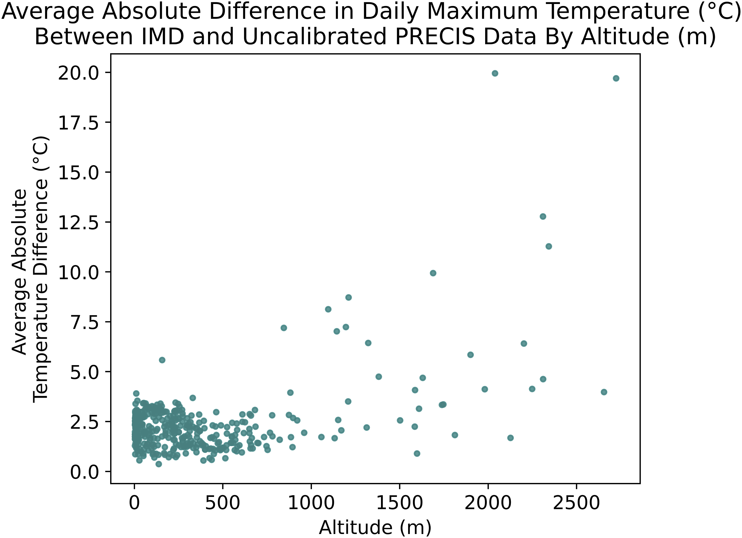
Figure 1 (right) shows that while the two datasets broadly agree, there is a mild cold bias in the first six months on average. Figure 1 also shows that while the average temperature difference in many locations is small, some locations have much larger (> 10°C) differences. In such cases, it can be argued that the original PRECIS data may be so unrealistic that even calibration may not produce reliable results. Figure 2 shows that these large differences in average daily maximum temperature occur almost exclusively in locations with altitude greater than 1000 m. Similar patterns can be seen in other variables. As such, we have decided not to produce any files for locations at elevations greater than 1000 m, thus rejecting data for 1134 locations (i.e. 19% of the raw data). We thus obtain a dataset size of 4790 locations with an altitude over mean sea level of less than 1000 m. A procedure was then created to calibrate these remaining PRECIS data with the IMD data. Left: Locations for which calibration data were obtained from the Indian Meteorological Department (IMD)
21
in the form of monthly climate normals over the 1981 - 2010 period. Each location was carefully checked for consistency and coordinates were corrected as needed. Right: Deviations in monthly mean daily maxima between IMD and raw PRECIS equivalents, suggesting the need for calibration. Absolute Difference Between IMD and raw PRECIS equivalent, averaged over months, plotted against the IMD recorded altitude of the location.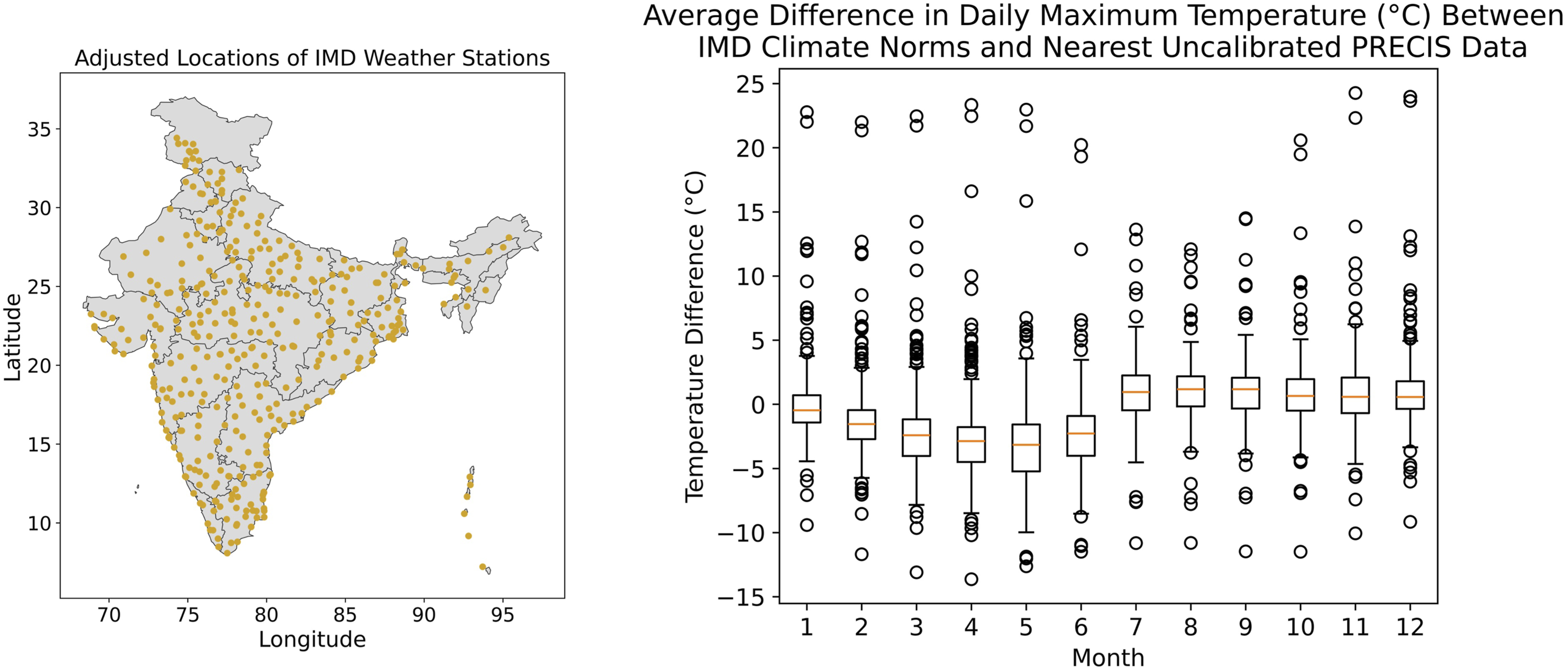
Methods
Here, we describe our methods in detail starting with basic data processing followed by decomposition and calibration of the solar data. Next, we show how the sparse IMD data for 400 stations described earlier can be used to calibrate high-resolution data (PRECIS, 4790 locations) for the remaining variables. Finally, using the calibrated data, we created TRYs using algorithms based on the well-known Finkelstein-Schaeffer statistic15,22 for dry-bulb temperature, relative humidity, wind speed and global horizontal irradiation. These processes gave us one TRY for each of the seventeen ensemble members of PRECIS. We then use a ranking procedure to generate our probabilistic TRYs from these.
Data processing
For each year and location, the PRECIS data consists of 360 days, corresponding to 12 months of 30 days each. To construct a 365-day year, the 30th day of each month is repeated where necessary from May onwards. No repetition or deletion was performed from January to March – both PRECIS and the Gregorian calendar consider this period to last 90 days, so the first 90 days from PRECIS were kept.
Where the 31st day in a month was constructed by repeating the 30th day, we decided to smooth the transitions between the days, following previous work suggesting the replacement of data between 10 pm and 1 am (inclusive) with data linearly interpolated between the 9 pm and 2 am values. 23
Some variables were converted to be in the units required for building simulation (i.e. the EPW file format). For example, dry-bulb temperature was converted from Kelvin to degrees Celsius and wind direction, which is in the interval [-180°, +180°] in PRECIS, is converted to the interval [0°, 360°] by adding 180°.
Snow depth in cm,
Infrared radiation and cloud cover was only provided every three hours in the PRECIS data, so we linearly interpolated between the reported values to obtain the missing data.
Solar data
The three hourly solar data provided in PRECIS represent surface downwelling shortwave flux in air, which we take to be equivalent to Global Horizontal Irradiance (GHI). For each time point, PRECIS estimates GHI by calculating GHI one hour before and after time
However, the result may not make sense at a given time. For example, suppose the underlying model GHI on a given day at hour
Returning to
For this reason, we add a processing step to the data. Let
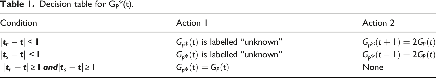
Decision table for GP*(t).
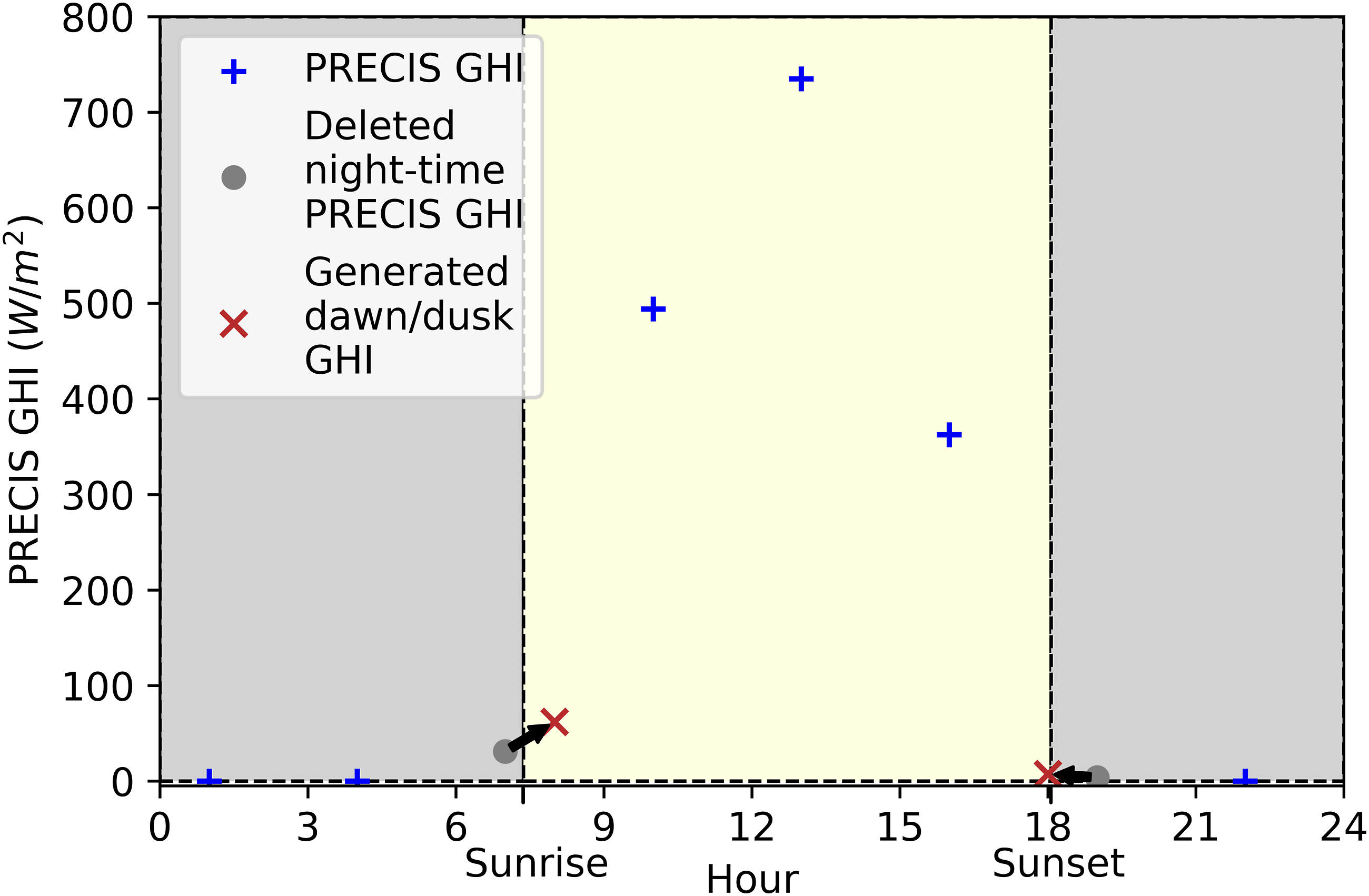
PRECIS GHI vs time at 23.17 N, 72.68 E (near Ahmadabad), ensemble 0, January 1st 1981. Unrealistically high night-time values (grey) are zeroed and replaced with values twice as large one hour earlier or later, as appropriate (red).
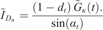
Energy simulation software programmes like DesignBuilder do not use Global Horizontal Irradiance directly, but rather diffuse horizonal irradiation (

To estimate 
The coefficients 
The variable
For solar calculations of variables such as
We began by estimating clear-sky GHI using,
30


We estimate 


We do not have the images to create 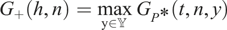
To obtain the calibrated GHI estimate, 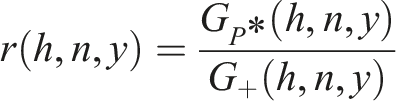

At these times when this 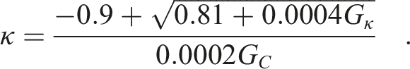
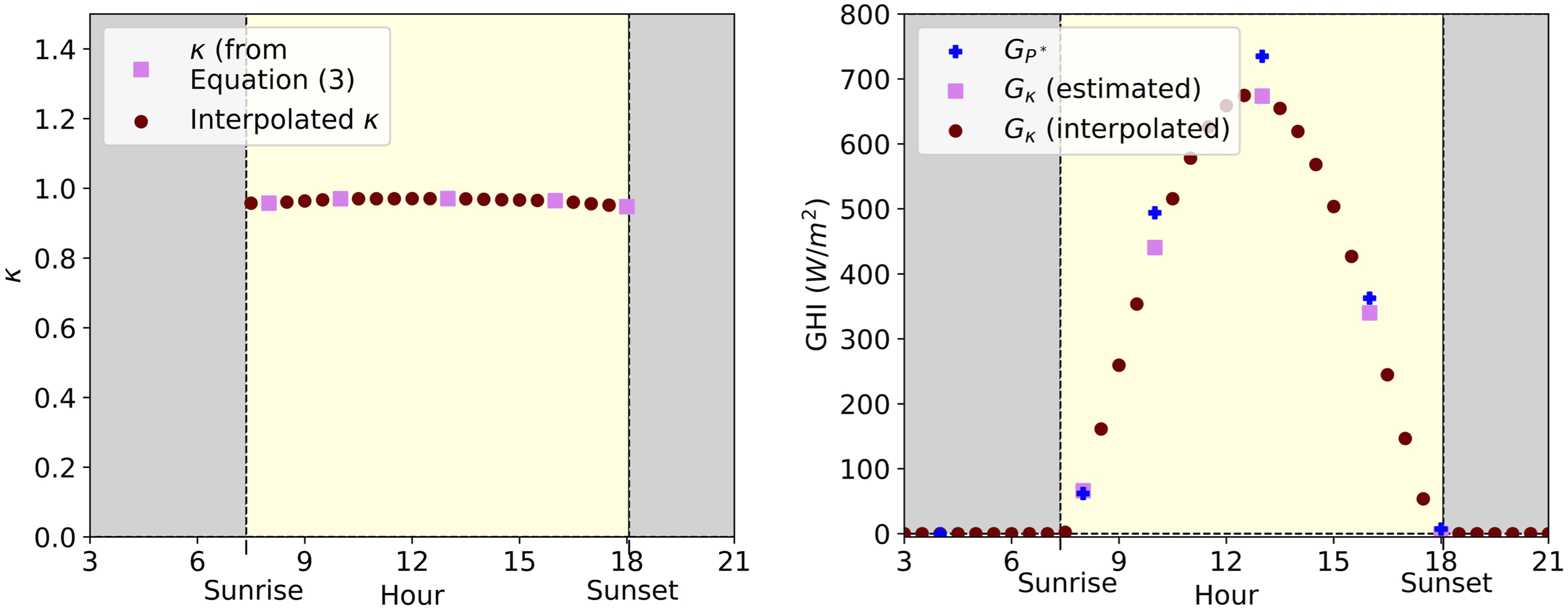
To obtain Clear-sky GHI, Left: Estimated We estimate the area under the curve of 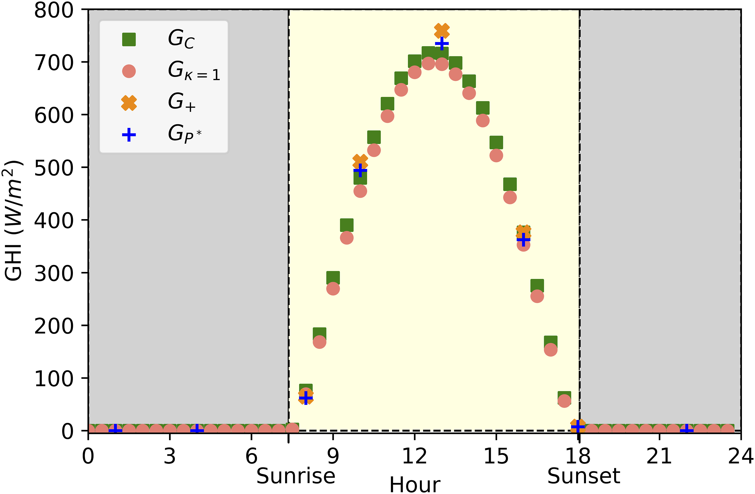
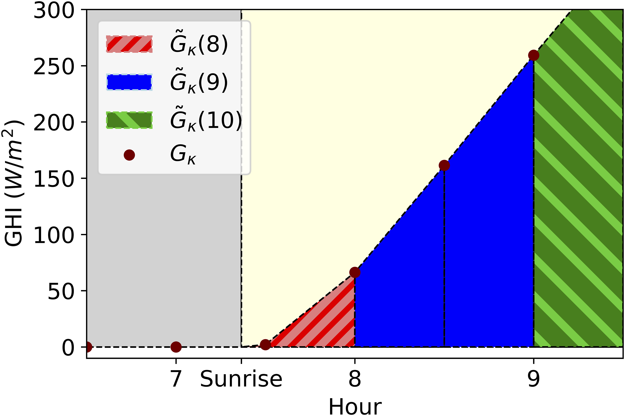
Given these half-hourly estimates of Global Horizontal Irradiance, the next task was to estimate the Global Horizonal Irradiation, which is the integral of Global Horizontal Irradiance over time, or the area under the Global Horizontal Irradiance curve. Since our values of GHI were not created using an analytic curve, we use the integral technique known as the trapezium rule to approximate the shape under the curve for each half-hour by a quadrilateral. To obtain the Global Horizontal Irradiation for each hour, we simply summed the estimated Global Horizontal Irradiation for each half hour.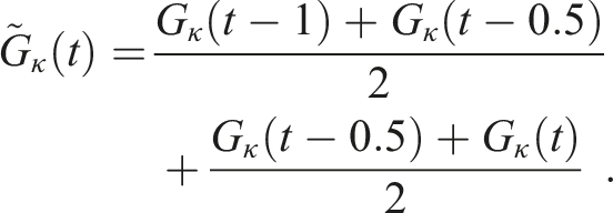
Given the values 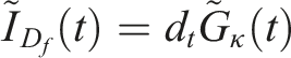
As a final step, if the mean Global Horizontal Irradiation during daylight hours for any day is less than 50 Wh/m2, the solar data is assumed to be in error and is replaced by the solar data from the previous day.
Calibration of non-solar PRECIS data
We wish to calibrate the PRECIS data using the known climate norms for 400 locations contained in the openly available IMD data set. 21 Here, we demonstrate how calibration coefficients for temperature, wind speed and relative humidity can be obtained for each of the 4790 locations depending on the difference between the PRECIS data and predictions based on the IMD climate norms.
Temperature – Interpolating norms
Of the 400 IMD locations, 6 were ignored as they were on outlying islands beyond the scope of our files, and one New Delhi location was deleted as its data differed substantially from two other New Delhi locations, and its provenance could not be established.
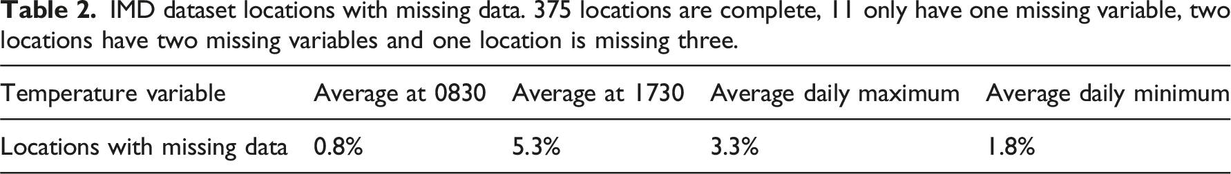
IMD dataset locations with missing data. 375 locations are complete, 11 only have one missing variable, two locations have two missing variables and one location is missing three.
In our interpolations we must account for the fact that air temperatures are known to decrease by an environmental lapse rate of between 0.6 to 0.9°C / 100 m. Hence, we begin by estimating sea-level temperatures by applying the environmental lapse rate of 0.6°C / 100 m in both the PRECIS and IMD data. After interpolating temperatures, we will re-apply the environmental lapse rate to obtain altitude-appropriate temperatures.
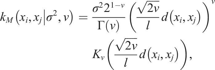
Given the existence of some missing data fields in the IMD source, as above, a choice to calibrate or not presents itself. Not calibrating, i.e. partial calibration using only the available series for a given location, risks leaving a part of the PRECIS dataset at odds with reality. However, the only means to calibrate, given missing fields, is to use data from a nearby location which may not share climatic characteristics with the location in question. To overcome this, we use a multi-output Gaussian process (or multivariate kriging) to estimate the minimum, maximum, morning and afternoon sea-level temperatures in each PRECIS location, using 35 ’s coregionalization approach. This allows us to model not only the spatial structure of each variable, but also the correlation structure in areas where one or more variables are missing. The assumptions and mathematics of this method are described after first contrasting against a single gaussian process.
In a single output Gaussian process, the values of a random variables 
It is also common to add a white noise kernel, or “nugget effect” to the kernel to avoid overfitting.
However, if we use a single separate Gaussian process for maximum and minimum daily temperature, for example, our estimates of minimum daily temperature near a site with daily minimum temperature would not take into account the known nearby maximum daily temperature, resulting in an unrealistic estimate. In contrast, the coregionalization approach to multiple output Gaussian processes described by,
35
uses a multiple-output kernel of the form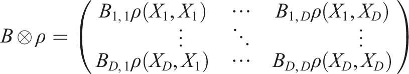
The value
In this way, the parameters of the kernel function
To jointly model average daily maximum/minimum and morning/afternoon temperatures, we fit a four-dimensional Gaussian process with a Matérn covariance function. We compared the predictive accuracy of this method with two other approaches. First, we compared the predictive accuracy of the model with simply using a 1D Gaussian process for each of the four temperature variables. This was performed using k-fold cross validation with k = 5. To do this, we began by stratifying the data into 5 equal segments. For each segment in turn, the model was trained on the data found by omitting one segment and tested by measuring the MSE of the model predictions with the observations in the fifth segment. MSE was then average across all five iterations.
We also compare our above approach against a simple linear interpolation approach to estimate the temperature norms. We do this by first creating an optimal triangulation mesh using the Delaunay criterion on the IMD locations followed by linear barycentric interpolation to estimate values in between.
MSE [°C] for different methods of predicting IMD norms.
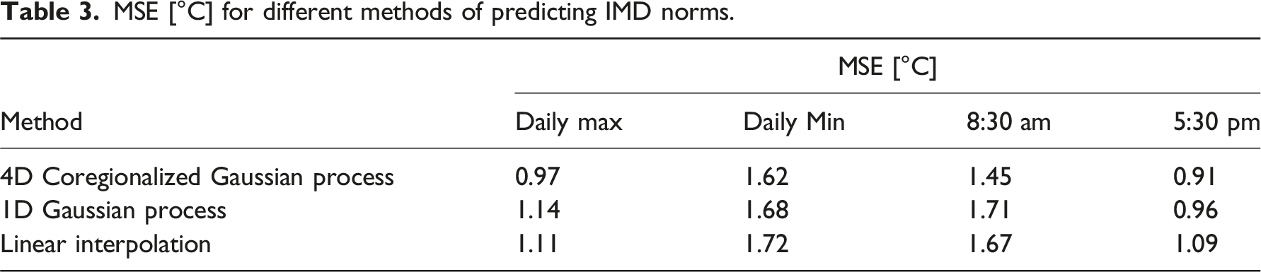
Figure 7 shows the results of the predictions for mean daily maximum temperature in the summer (April – June). The “sea-level”/normalised predictions are extremely smooth across the country, whereas the final predictions in the right-hand plot take into account the local topography better (c.f. elevation data in Figure 7). Top Left: Average summer (April-June) daily maximum temperatures for all Indian locations <1000 m above mean sea level (grey otherwise). “Sea-level” temperatures refer to Gaussian process predictions. The top right-hand plot gives temperatures after the lapse rate of −0.6°C/100 m has been applied used to calibrate our data. The bottom left plot shows elevation above mean sea level.
Temperature – calibrating values
The approach of the previous section has given us estimated daily temperature maxima and minima at each of the 4790 locations under consideration. Given these estimated daily maxima and minima for each month 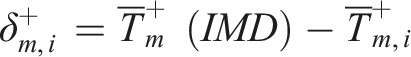
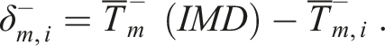
Given these average daily extremes for each month, two different approaches to calibrating temperatures were hence adopted depending on whether the average diurnal range was being made wider (
If 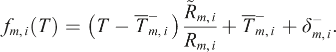
It is algebraically straightforward to prove that
If 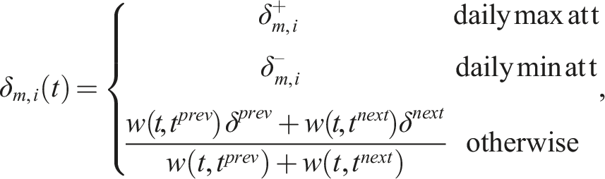
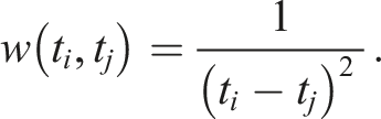
The temperature shift
Wind speed
When calibrating wind speed data, it is important to ensure that the speeds remain positive. For this reason, we use a multiplicative scaling factor on the PRECIS wind speed data to ensure a match with the IMD climate norms data.
We begin by interpolating the IMD wind speed data between locations using a one-dimensional Gaussian process with Matern covariance function (after converting IMD data from km/h to m/s), and calling these values 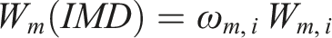
Figure A2 shows the RMSE for a ‘leave one out’ analysis of our wind-speed data. We note that the basis data for wind speed, in general, are very poor as noted in 6 and hence the somewhat high RMSEs observed here are not seen as being of concern.
Relative humidity
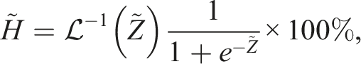
It was similarly important to ensure that relative humidity values remain between 0 and 100%. As such, before calibrating we first transform the domain of the humidity data from 
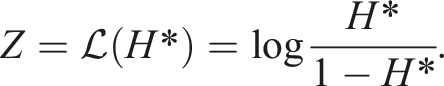
Our IMD data provides average relative humidity in the morning, at 0830 hours, and in the afternoon, at 1730 hours. In month 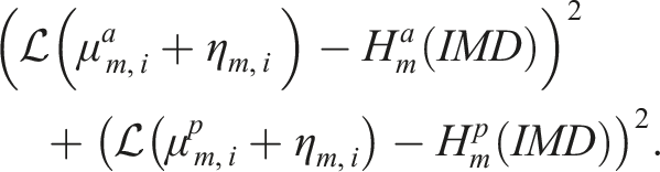
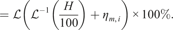
Given these values, the calibrated relative humidity 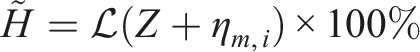
After this calibration, we occasionally find some days with unrealistically low relative humidity. Hence, when the average relative humidity for a day is less than 20%, we delete all of the data from that day and replace it with the data from another day within 10 days, selected at random. Figure A3 shows the RMSE for a ‘leave one out’ analysis of our humidity data, with a small positive bias.
After calibrating each month in every variable, transitions between the months are smoothed using the method given in. 23
Finally, we must estimate the dew-point temperature 


All calibration coefficients are used for current and future climates through the assumption of stationarity, as it is unknowable whether these would change and how.
Production of calibrated TRYs
We adopt the well-known procedure detailed in BS EN ISO 15927-4:2005,
15
to construct a Test Reference Year (TRY) for each calibrated ensemble. In summary, for each month of the year, the Finkelstein-Schaefer statistic
22
was used to find the most typical month from across the 30 years of data. The value of the empirical cumulative distribution function (CDF) for an observation 
For each month and year, we calculated the weighted average of the FS-statistic for dry-bulb temperature, relative humidity and Global Horizontal Irradiance, and find the three years with the lowest resulting value. From these years, we select the year with the lowest FS statistic for wind speed and used this to provide the month’s data for our TRY for that ensemble.
As there are seventeen ensemble members, this procedure results in seventeen TRY files for a given location and given set of basis years for current (1981-2010) and future (2060-2089) climates.
Construction of pTRYs
Given the 17 TRYs created, the probabilistic TRYs are created using the procedure described in. 39 For each month, the TRYs are ranked according to a single variable. We have selected average dry-bulb temperature as this is considered most important for a building’s energy performance. To select a month to use in a pTRY, the 17 different TRYs are ranked by dry-bulb temperature for that month. To create a 50th-percentile pTRY, for each month, the full weather data from the 50th percentile month from the TRYs are chosen. The transitions between the months are then smoothed as before, and the dew-point temperature is recalculated.
Calibrated thermal model
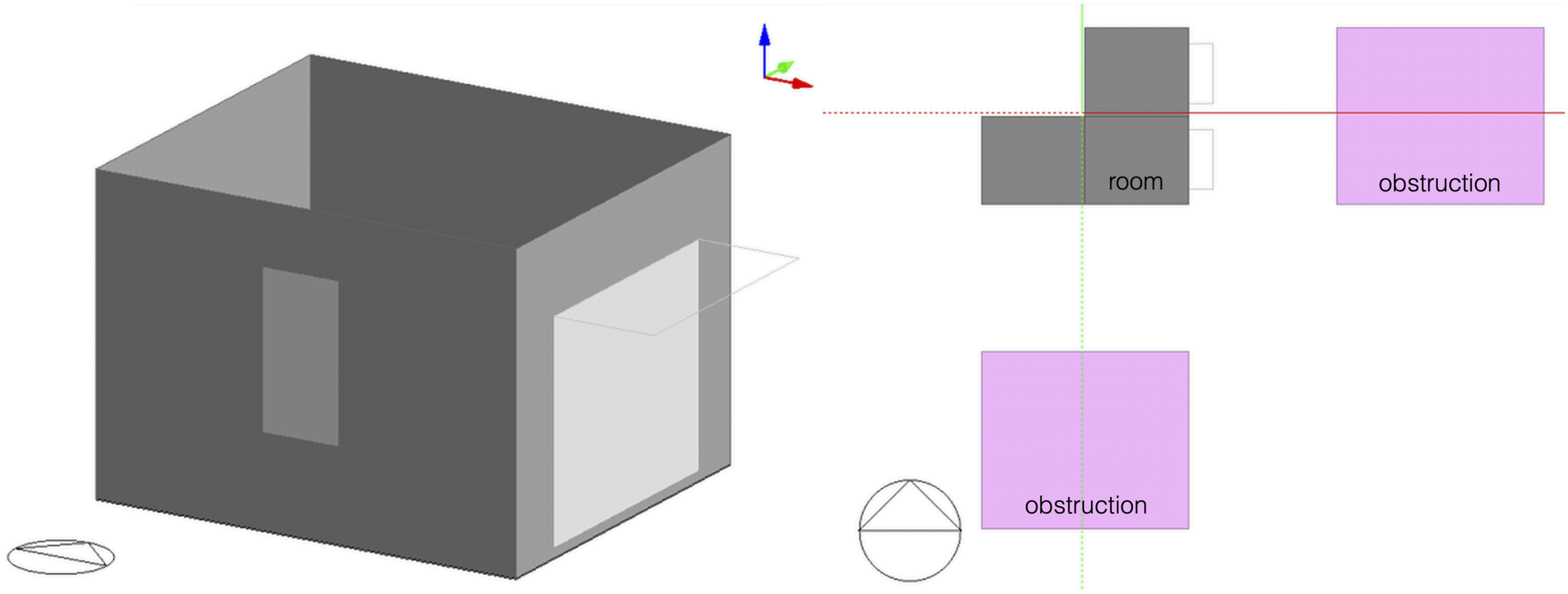
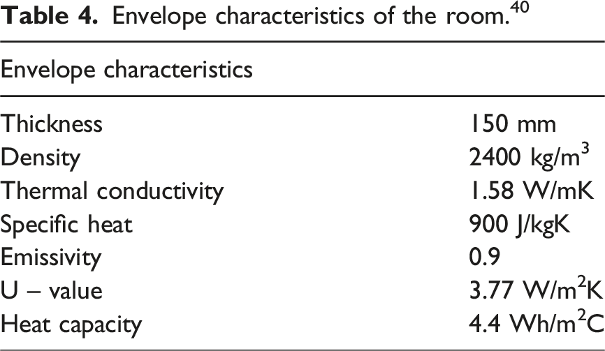
To show both the use of the pTRYs developed and to make a brief examination of the impact of future climates on indoor temperatures and energy demand, a calibrated thermal model of a typical building in India is needed. A model of a room pre-calibrated to indoor dry bulb temperature in free running operation (CVRMSE 7.5%), in a typical apartment dwelling in Ahmadabad was available via.
40
Modelling was undertaken using DesignBuilder v7.2 built on the widely used EnergyPlus engine (v22.1). Indoor and outdoor dry bulb temperature measurements were available for a summer period (30 May – 6 June), and the model calibrated. The model views and envelope characteristics are provided in Figure 8 and Table 4. See Appendix 2 for further inputs and calibration detail. The indoor temperature for free running buildings and energy use intensity of an air-conditioned variant are assessed. Axonometric view of the room model on the left. The plan view on the right shows the room in context of adjacent rooms above and to the left (in grey) with both the external walls facing adjacent buildings (in pink) 6 m away. Envelope characteristics of the room.
40
Results
Figure 9 visualizes the annual average outdoor dry bulb temperature, for the historical and future data for the 50th percentile TRY, and their difference. All the plots display a clear geographic pattern, and the difference map shows that the increase is greater in the northern plains and central India of around 3.75°C compared to around 2.25°C in the coastal southern regions. Looking at summer conditions when the effect on indoor temperatures and consequently energy consumption is highest, it is apparent that locations with higher humidity experience smaller increases in dry bulb temperature. Annual outdoor average dry bulb temperature map; historical (1981-2010, top left) and future (2060-2089, top right) from the 50th percentile TRYs. The bottom left graph shows the difference between the two (positive numbers indicate future is warmer). The bottom right graph shows summer data (taken as March to June) through a scatter plot of the difference in mean dry bulb temperature (positive numbers indicate future is warmer) and the historical mean relative humidity.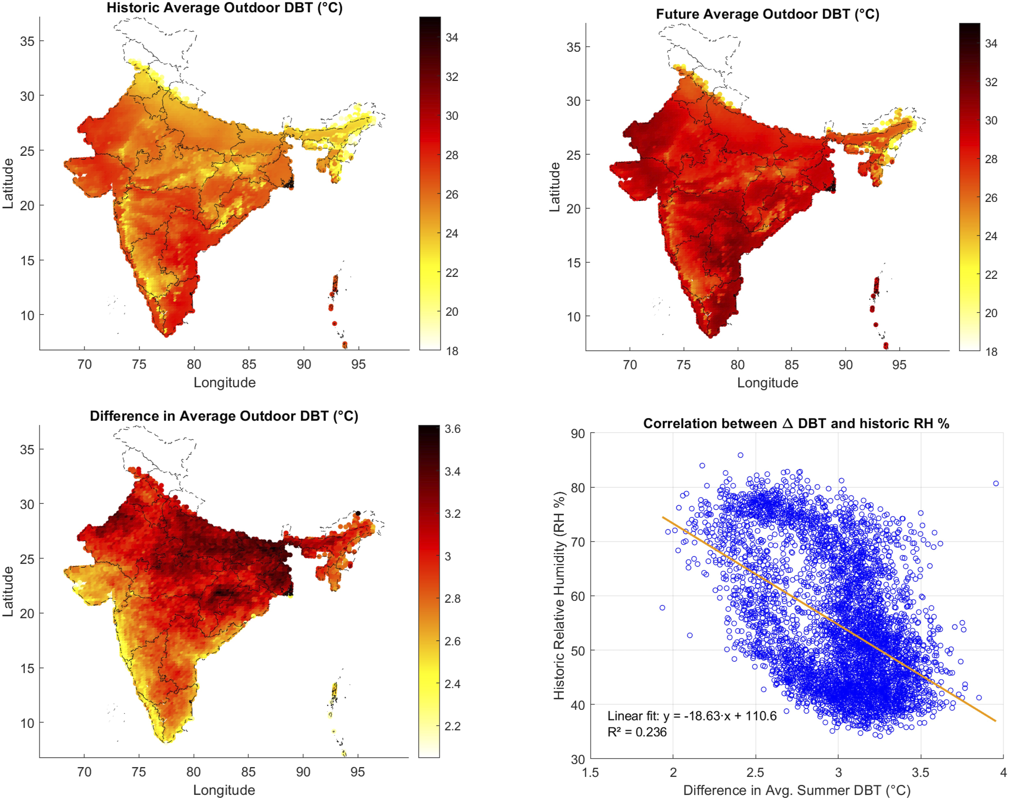
Figure 10 shows the outdoor peak (i.e. 1-hour) dry bulb temperatures for India, based on historical and future weather data respectively, and the difference plot. Unlike the annual average data, the geographic signal is weaker in these data. A majority of locations (96.7%) show an increase in peak temperatures with a mean increase in these locations of 2.97°C (s.d. 1.44°C) and a max of 8.2°C. In contrast, 3.3% locations show a drop in the annual peak temperature with a mean decrease in these locations of −0.75°C (s.d. 0.75°C) and minimum of −4.6°C. This is consistent with the TRY method in that the selection is on the representativeness of the months rather than peak temperatures. This is already visible in the difference plot of Figure 9 where no location shows a fall in annual mean temperatures. Peak (1-hour) dry bulb temperature map; historical (1981-2010, top left) and future (2060-2089, top right) from the 50th percentile TRYs. The bottom left graph shows the difference between the top right and top left, excluding outlier data (i.e. positive numbers indicate future is warmer). The bottom right graph shows the equivalent difference for the 90th percentile TRY files.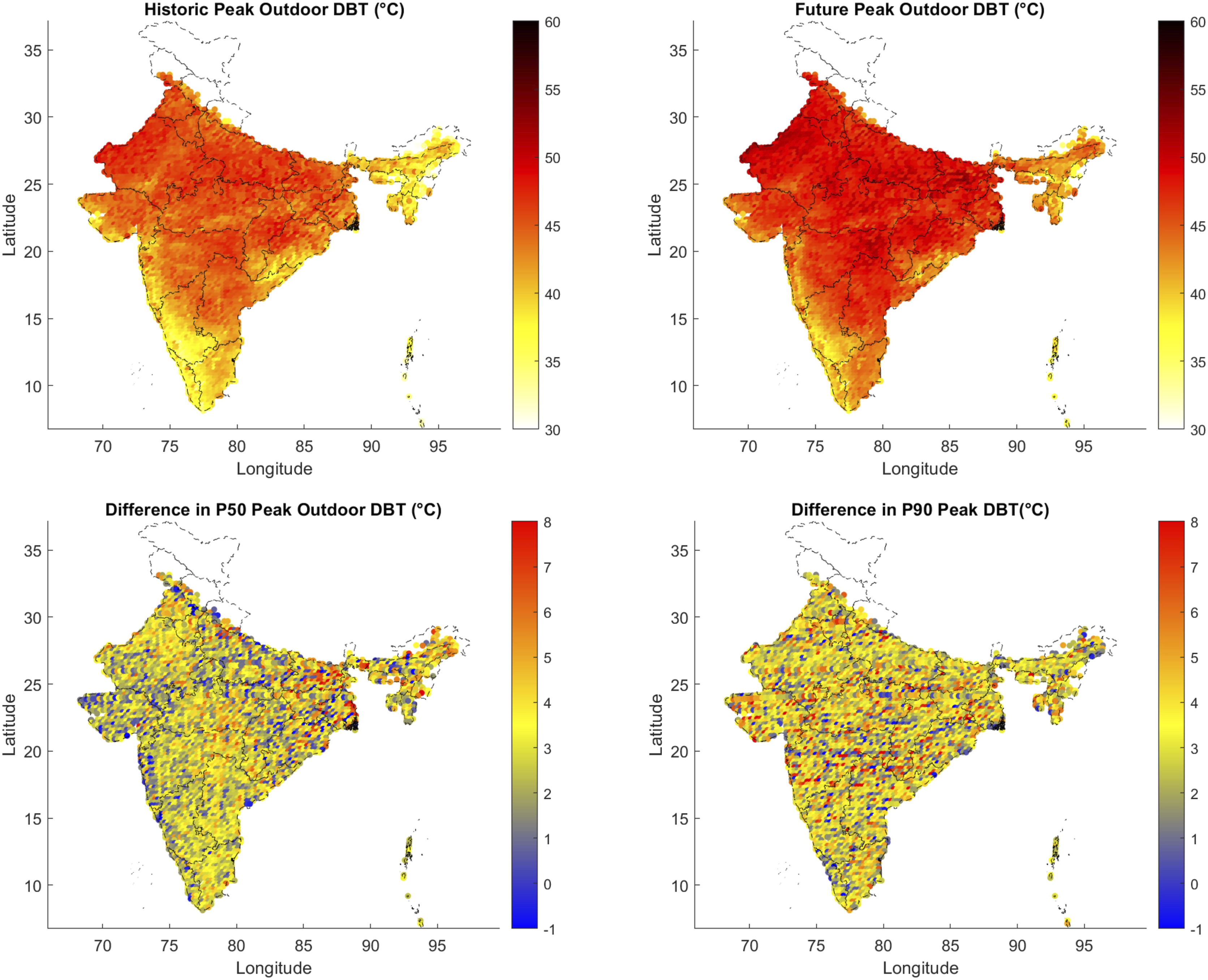
Figure 11 displays these metrics for six climatically different cities across India. Future values are seen to be greater than historical in all instances, except for Mumbai’s peak outdoor air temperature which is nearly identical for current and future, though mean outdoor and indoor temperatures have risen. Historic and Future metrics for six climatically different cities across the country.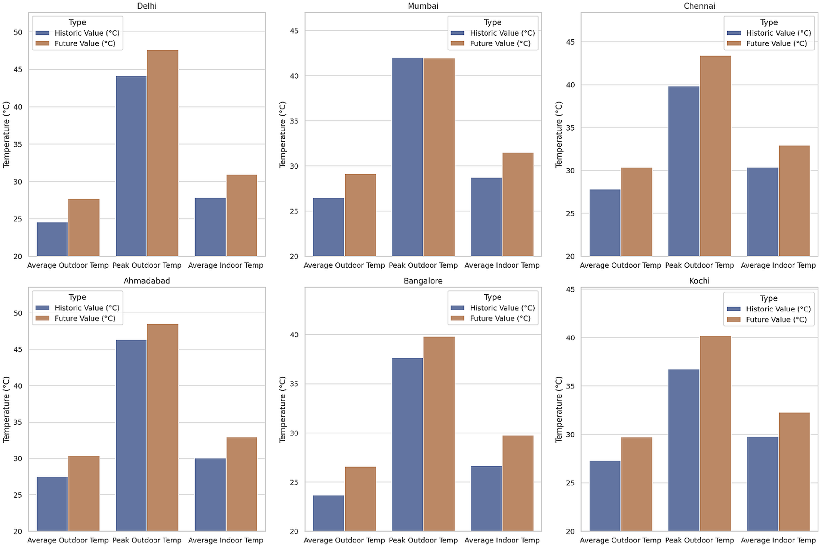
Impact on indoor temperatures and energy use
Free running and air-conditioned variants of the calibrated model were used to simulate the indoor air temperature and cooling Energy Use Intensity (EUI), respectively. The indoor air temperature displays a pattern very similar to that of the average annual outdoor air temperature, with an increase in the range 2°C – 4°C between the historical and future data with an all-location mean of 3.05°C (s.d. 2.03°C) (Figure 12). We observe that the existing underlying geographical patterns are maintained with climate change with the eastern parts of the country expected to see the most significant increases in indoor temperature. Annual indoor average Temperature map; historical (top left) and future (top right) and difference plot (bottom, future - current) using the 50th percentile TRYs.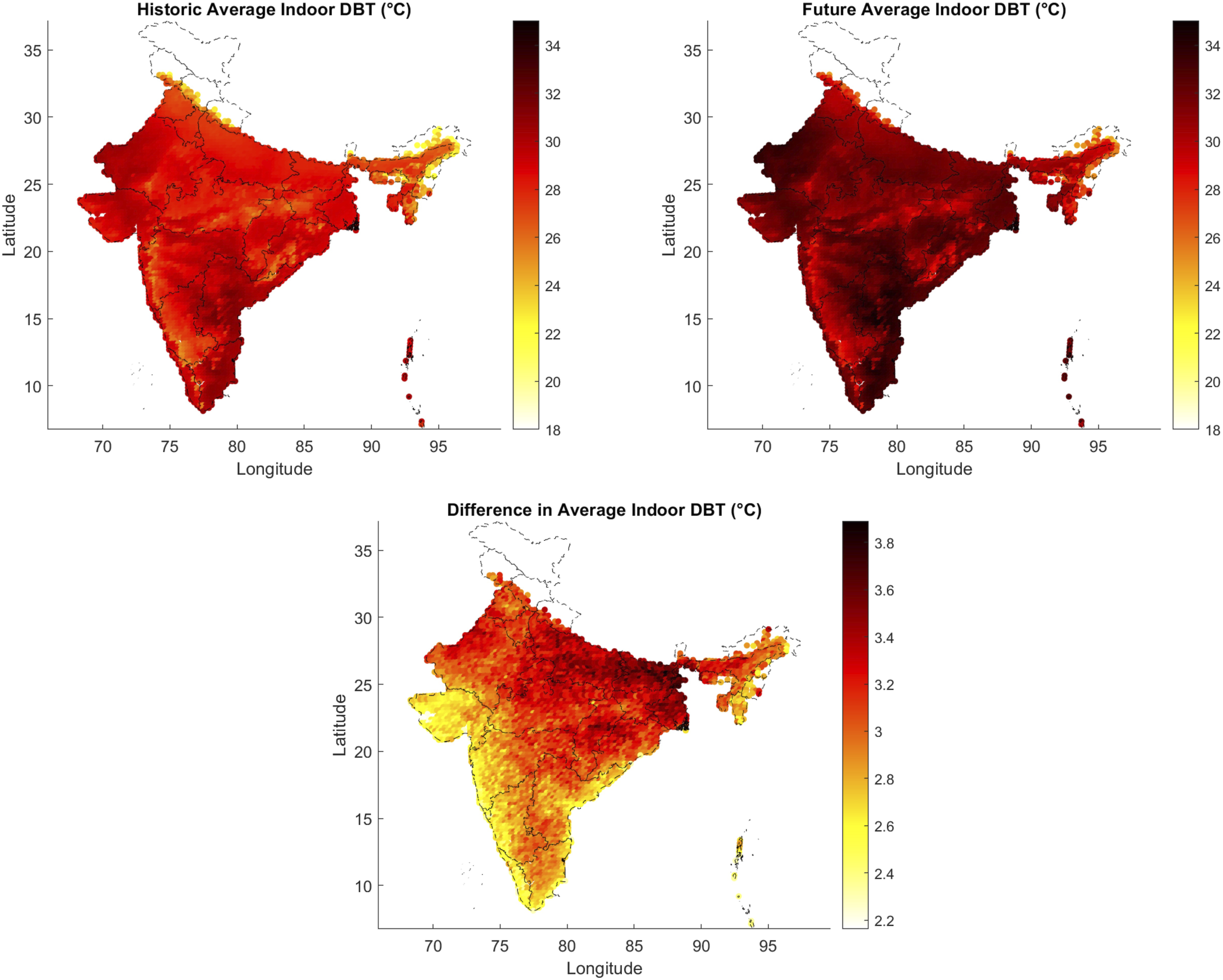
EUI results for the conditioned area (i.e. a bedroom) are shown in Figure 13. The left side of the figure uses historical weather data, while the right side predicts future conditions. In our calibrated model we obtain an EUI of 98 kWh/m2/a, for the conditioned area under current climate. This is broadly consistent with data on “households with more than two air conditioners or more than four occupants” with an EUI of about 80 kWh/m2/a, though considerably higher than the mean of around 50 kWh/m2/a, for this location.
41
We consider this acceptable given that absolute demand is rapidly increasing over time as incomes rise, access to air-conditioning increases and unit costs fall
41
and that our main interest is in the differences between present and future. Annual cooling energy use intensity (EUI) map; historical (top left) and future (top right) and difference plot (bottom left, future - current) for the 50th percentile TRYs. The bottom right graph shows the split of latent and sensible daily energy use in 10 kWh/m2 bins from the difference plot.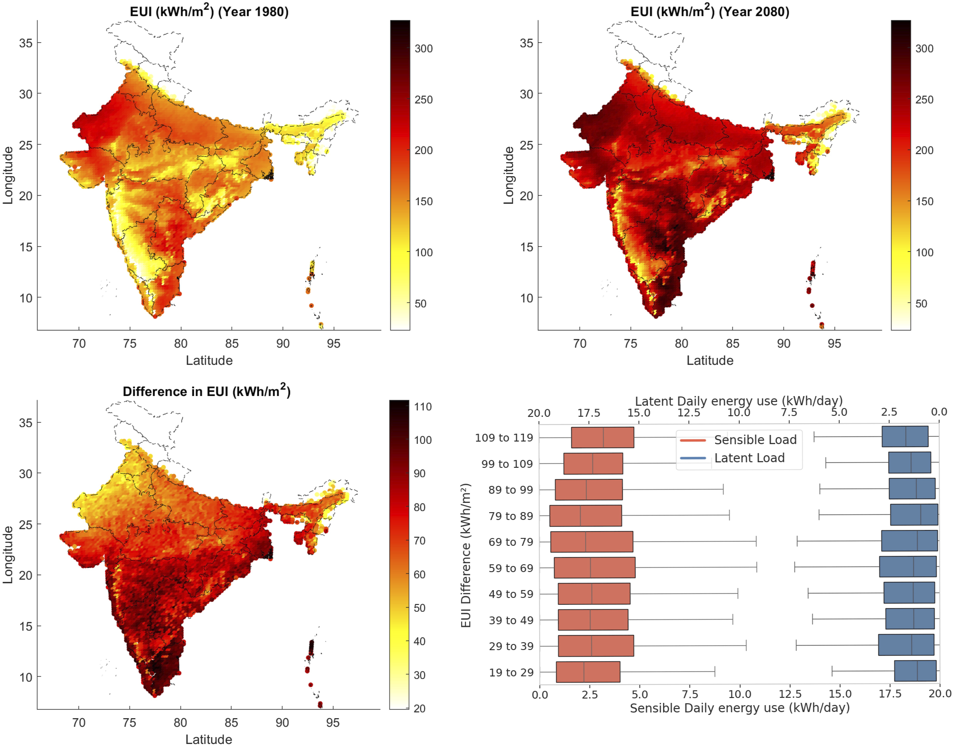
We observe that the increase in EUI pattern is different to that observed for the indoor and outdoor annual average temperatures given that the greater increase in EUI is in the south of the country, rather than the east, with an all-location mean increase of 74.8 kWh/m2 (s.d. 14.9 kWh/m2) from a base of from 147.5 kWh/m2, i.e. a 51% increase over the studied period. While a small increase in daily sensible cooling energy demand is suggested for those areas with the highest rises in overall EUI, the overall sensible and latent changes are secularly distributed across the difference bins.
Discussion
While weather data drawn from observed data are increasing, and industry bodies such as the simulation software company DesignBuilder are in the process of aggregating a disparity of sources, 42 there continues to be a clear need for localised weather data for building design and simulation, especially in the global south. Previous work in the UK, and the present work applied to India, are examples of how synthetic data can meet these requirements. Compared to observed hourly data which, apart from being geographically sparse, suffer from data quality issues (e.g. the lack of good solar data and the lack of continuous observations over 30-year periods), synthetic data have the advantage of being continuous, consistent between now and the future and generally complete.
However, these data are not without their substantial challenges especially in establishing ground-truth. Here, we have presented a series of methods to improve data validity that can be replicated for calibration elsewhere, provided a suitable sparse data set based on observed data is available. In this instance, the sparse data set comprises monthly climate normals for around 400 locations. Using these, we elaborate a method to scale the calibration data to 4790 locations for India. We show that the 4D Coregionalized Gaussian process has a significantly lower error rate than the simpler 1D Gaussian process and linear interpolation. Solar data present a different set of challenges due to the need to have hourly direct and diffuse irradiance in the weather file. We demonstrate a method that can be applied to decompose three-hourly global irradiance into these components. Of course, our work, in common with others in the field, assumes stationarity. It is hence possible that some weather parameters may behave differently in the future, e.g. a mass uptake of electric vehicles could change conditions such that solar radiation intensifies. These and other unknown complexities are left to future work.
Our results clearly demonstrate the localised nature of weather patterns and hence the need for their use in building design and simulation (see Appendix 4 for an example from the eastern state of Odisha). This is true even of locations that might otherwise share the same Köppen-Geiger climate classification. While temperatures are shown to increase in future, the deviations are location dependent. A small minority of locations (3.3% of our data set) experience a decrease in peak temperatures (up to −4.6°C), the rest (96.7%) see substantial increases with some locations expected to see peak temperatures go up by 8°C.
Figure 14 shows the first week of June (pTRY50) indoor and outdoor temperature time-series for two locations: Jaisalmer, a town in the North-West (NW) desert region, and Chennai, a city in the south-east (SE) and close to the tropics. These usefully illustrate why the SE of the country is seen to contain the greatest EUI differences in Figure 13. The outdoor night-time minima in historical Chennai regularly drop below the set-point temperature, whereas this is much less true of the future whilst also being accompanied by greater daytime peaks. Thus, the difference between the mean set-point and mean daytime peaks increases substantially in the future in Chennai (+1.2°C) compared to Jaisalmer (+0.8°C). Temperature time-series for the first week of June showing the outdoor air temperature, indoor air temperature for the naturally ventilated (NV) and air-conditioned (AC) cases of our calibrated room and the IMAC-R operative set-point temperature. Historical data are in the left column and future data in the right column. Jaisalmer (NW) is shown in the top row and Chennai (SE) is in the bottom row.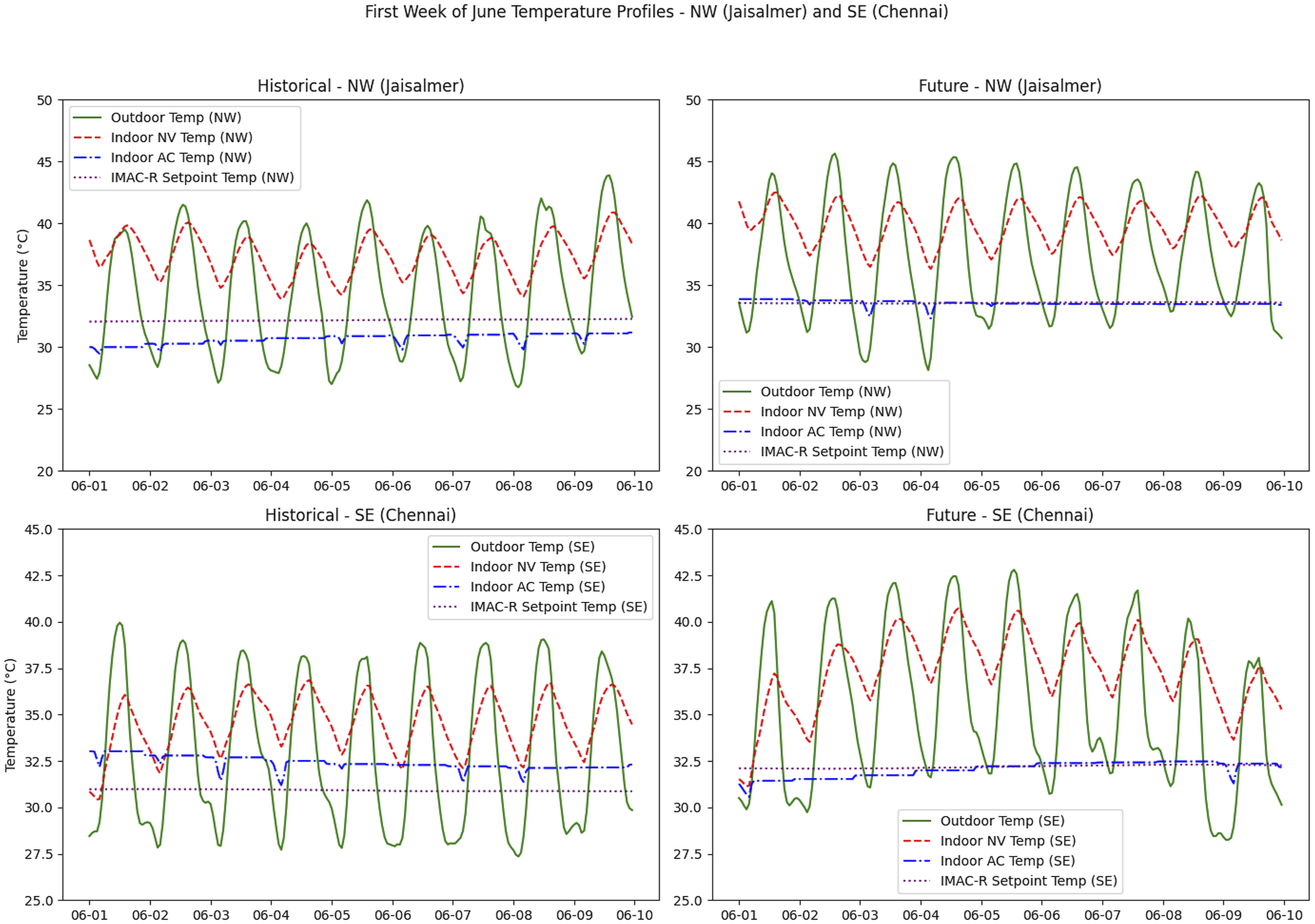
It is noteworthy that even a modest increase in peak temperatures in an otherwise humid location can have a substantial impact on human health and the resilience of power systems to cope with the associated increase in air-conditioning demand. Taking a simple example, a dry-bulb temperature of 32°C at 75% relative humidity is a wet-bulb temperature of 28.3°C, which increases to 30.2°C at a dry-bulb temperature of 34°C at the same relative humidity. Thus, a ‘small’ shift in dry-bulb temperature has moved the wet-bulb temperature to above 30°C, a situation of potentially serious heat stress for even young healthy adults. 43 Knowing the localised potential risk of such heat stress is therefore critical in designing buildings that will provide healthy indoor environments well into the future.
Conclusions
In this paper we present a new approach to producing reliable current and future weather data for use in building performance prediction, but with the potential for wider applicability in other areas such as infrastructure or crop resilience. By studying the case of a large developing country like India, with very little data presently available compared to its size, we show that it is possible to reliably convert data from a global climate model (PRECIS) at 25 km spatial resolution and use geographically sparse time-aggregated ground truth data to produce mutually consistent hourly weather data for historical and future periods.
It is known that data at such spatial resolution reduces the potentially significant errors in predicting critical building performance indicators such as energy use intensity and indoor temperatures. Predictions of high fidelity are needed given that between 17% – 22% of global carbon emissions are directly linked to the need to heat and cool buildings and that humans spend 90% of their time inside buildings, necessitating the creation of a thermal stress free and comfortable indoor environment.
Our results clearly show the benefit of such a highly local representation of weather with visible differences in prediction for adjacent grid cells throughout India. The urgent need for mutually consistent future weather data is also apparent given typical building lifetimes of around 60 years and the significant increases in cooling energy use intensity predicted for many parts of the country, with a mean increase of 51%. Poorly designed buildings especially in places that cannot afford air-conditioning could see significant increases in hot indoor conditions, up to 4°C hotter in many locations in the 50th percentile case, leading to heat-stress linked morbidity and mortality. It is noteworthy that these are predictions for typical conditions, not extremes such as heatwaves, which will be much hotter.
All our produced weather files are available in a free to access and use public repository (see acknowledgements). Basis data, such as PRECIS used in this work, are increasing in availability and reducing in cost; the approximate cost of production in this case being just £5 (∼ ₹ 500) per weather file, including data and person-hours. In light of the potential savings in energy, carbon, health and well-being from just one building per grid location, these data can be seen as being practically “free” to produce. We hence hope others will be able to replicate our method and, by doing so, incur even lower production costs. The new method is globally applicable and will hopefully lead to the worldwide production of such files, particularly in the global south.
Footnotes
Acknowledgments
In producing this work, we would like to gratefully thank Nick McCullen (University of Bath), Francesca Cecinati (Artesia Consulting), Lorna Wilson (Clarks), Woong June Chung (Gachon University) and Titas Ganguly (IIT Roorkee) for their contributions. We are also grateful to Andy Tindale (DesignBuilder), Nishesh Jain (DesignBuilder, PSI Energy), Gaurav Shorey (PSI Energy), Kartik Amrania (SWECO), Rajan Rawal (CEPT), Yash Shukla (CEPT) and Dru Crawley (Bentley) for testing the weather files at various stages and their useful comments. This work was funded through the DST (DST/TMD/UK-BEE/2017/17) and EPSRC Zero Peak Energy Building Design for India (ZED-I, EP/R008612/1). The generated files can be downloaded from ![]() .
.
Author contributions
Declaration of conflicting interests
The author(s) declared no potential conflicts of interest with respect to the research, authorship, and/or publication of this article.
Funding
The author(s) disclosed receipt of the following financial support for the research, authorship, and/or publication of this article: Engineering and Physical Sciences Research Council, EP/R008612/1, Department for Science and Technology, India, DST/TMD/UK-BEE/2017/17.