Sage Journals: Discover world-class research

Abstract

Direct load control (DLC) for building HVAC systems, through preconditioning and setup/setback sequences, can substantially reduce electricity consumption during peak periods. Yet, the effectiveness of a DLC sequence strictly depends on the thermophysical attributes of a building and its occupants’ tolerance to variations in the thermal environment. The current one-size-fits-all approach to DLC disregards the inter-building diversity of these factors. This paper demonstrates the inter-building diversity of preconditioning and setup/setback needs by deriving unique DLC sequences for different buildings. To this end, variants of an EnergyPlus model representing a small commercial building in Toronto, Ontario are created by altering its envelope, HVAC capacity, and occupants’ temperature preference characteristics. Through a metaheuristic search, personalized DLC sequences that minimize the HVAC-related electricity costs and the time spent outside a preferred temperature range are estimated for each variant. These personalized DLC sequences were compared with six baseline DLC sequences. Unlike the baseline DLC sequences, the optimal sequences could attain an average of 20% reduction in HVAC-related electricity costs while keeping the time spent outside the preferred temperature ranges under 3% for all variants.

Practical application

This paper presents an optimization method to derive unique direct load control sequences demonstrating the inter-building diversity of preconditioning and setup/setback needs. The method is tested on a range of buildings with varying characteristics in a simulation environment. The findings of the study are useful in the domains of HVAC controls, demand response, and electrification of HVAC systems.

Keywords

Direct load control global optimization HVAC systems control dynamic electricity pricing

Introduction

Electrification is the process through which end uses that directly or indirectly rely on fossil fuels are powered by electricity from non-emitting generation capacity.¹ The process commonly includes replacing gas furnaces, water heaters, and boilers with heat pump systems, conventional vehicles with electric vehicles, and coal and gas-burning power plants with renewable energy sources. While electrification has been regarded as the main pillar for the decarbonization of our society, it represents a major challenge for electrical grid operators due to an increase in demand accompanied by increased uncertainty in generation.

Demand-side management (DSM) has emerged as a promising solution to address the risk of a supply-demand mismatch through dynamic electricity pricing. Consumers either manually or automatically change their electricity use to avoid on-peak rates. If this change is executed algorithmically through automation, it is commonly referred to as a direct load control (DLC). A widely used DLC example is preheating/precooling prior to the start of peak events and curtailing heating/cooling during peak periods.

An overview of DLC for HVAC systems

Different DLC sequences have been used for a wide range of building typologies – school buildings,² office buildings,^3–6 shopping centres and retail buildings,^3,7 data centres,² laboratory buildings,⁴ and residential buildings.^8,9 Demonstrations of the technology have been completed in a range of ASHRAE¹⁰ climate zones and different utility jurisdictions – Zones 0 to four in various cities in Australia,² Zone 3 in Italy⁷ and China,⁵ Zone 4 in California,⁴ Oregon, and Washington,³ and Zone 6 in Ontario,⁶ Quebec,⁸ and New Brunswick.⁹

While some of these studies used simulation^2,5,7 or unoccupied laboratory buildings,⁸ others conducted field experiments assessing the performance of DLC sequences in occupied buildings.^3,4,6,9 Laboratory- and simulation-based studies had to rely on thermal comfort standards (e.g., ASHRAE Std. 55¹¹) to assess the impact on occupant comfort and satisfaction, which are not intended for transient thermal environments caused by DLC sequences and do not consider the broader effect of financial incentives due to dynamic electricity pricing on occupant behaviour. For example, ASHRAE Std. 55 limits temperature drifts or ramps to no more than 2.8°C for changes taking place over a two-hour period and 3.3°C for changes taking place over a four-hour period. These restrict how fast DLC sequences can recover from a setback/setup during a peak period.

Peak reduction potentials reported in the literature exhibit significant variation. This is partly because they are computed relative to a different baseline computation approach (i.e., an estimate of the demand without the DLC sequence).¹² Among the reviewed literature, only Piette, et al.³ reported savings estimates with respect to multiple baseline computation approaches; specifically, an outdoor temperature-based regression approach and two different day-matching approaches. Lack of a standardized baseline calculation approach poses a challenge to quantify the performance of DLC sequences. Simulation-based studies did not suffer from this limitation, as they have access to a perfect baseline in the form of a simulation without a DLC sequence. Another factor contributing to the variation in performance levels is the diversity of metrics reported.¹³ Metrics reported include electricity demand reduction, percent reduction in heating or cooling loads, or electricity demand by the HVAC systems. Further, these metrics can be calculated for the average, maximum, or minimum demand reduction sustained over a peak period.

The case for personalized DLC sequences

The effectiveness of a DLC sequence depends on the thermophysical properties of the building envelope, HVAC system sizing, and local climate. In line with this, Huang, et al.¹⁴ investigated the temperature response during precooling and setup periods in five different commercial buildings, and revealed that the temperature slopes during precooling were between −1°C/h and −5°C/h and the temperature slopes during setup were between 1°C/h and 5°C/h. Similarly, Markus, et al.⁶ conducted a field study in a 27-zone variable air volume (VAV) air handling unit (AHU) system implementing a DLC sequence with a two-hour and a 2°C precooling period followed by a 2°C setup. They observed that the temperatures rose to the setup temperature setpoints in nine of the zones in less than 2 hours after the beginning of a peak period. Perhaps more interestingly, temperatures reached the setup levels consistently in the same order, approximately at the same time during each unique peak period. This highlights that the precooling intensity and duration needs are unique, but predictable, for different spaces, and the DLC sequence parameters should be tuned to maximize demand flexibility.

Pardasani, et al.⁹ reported that while the majority of their 567 participant households did not find a 2°C preheating noticeable, some reported discomfort. Sarran, et al.¹⁵ and Khorasani Zadeh, et al.¹⁶ identified a significant inter-household diversity in occupants’ thermostat use behaviour during peak periods. Simply put, the range of acceptable indoor temperatures is different for different individuals, imposing building/zone-specific limits on the allowable intensities for precooling/preheating and setup/setback periods.

Motivation and objectives

Despite the aforementioned factors highlighting the need for personalized building/zone-specific DLC sequences, the majority of the DLC sequences tested employed generic and heuristics-based preheating/precooling intensities and durations typically between 1 and 2°C and 1-2 hours and setup/setback intensities typically ranging between 1 and 2°C. Model-based predictive control (MPC) represents a framework to optimize DLC sequences in real time to minimize the electricity cost with dynamic pricing. For example, Gehbauer, et al.¹⁷ employed non-linear programming to optimize temperature setpoints with time-of-use (TOU) pricing. Deng, et al.¹⁸ formulated an MPC algorithm using a thermal network model and quantum annealing to search for optimal temperature setpoints with TOU pricing. Chen, et al.¹⁹ employed the chaotic satin bowerbird algorithm and a neural network model to optimize temperature setpoints with TOU rate scenarios. Reynolds, et al.²⁰ also used a neural network formulation as a controller model and employed the genetic algorithm to identify the setpoints minimizing the electricity cost with TOU rates. Several other studies developed MPC algorithms for different dynamic pricing scenarios, climates, and building archetypes.^21–24 However, MPC algorithms for demand flexibility so far have found limited application outside research,²⁵ particularly in small commercial buildings.²⁶ This can be attributed to the fact that MPC development tends to have a high engineering cost,^27,28 which is expected to influence the initial cost for MPC software tools. In addition, integration of MPC algorithms, including configuration of a dedicated server and mapping BAS and external inputs and outputs, currently remains a labour-intensive task.²⁹ MPC deployments also require a modern BAS infrastructure, which is not always available in small commercial buildings. As a result, the benefits of MPC do not perfectly scale to small commercial buildings.³⁰

This paper develops a building performance optimization methodology to derive near-optimal ready-to-use DLC sequences for small commercial buildings. The gap that we intend to fill with this paper is a happy medium between complex model-based or model-free supervisory DLC algorithms and generic one-fits-for-all DLC sequences. We seek to answer two research questions: (1) What are the comfort and electricity cost reduction consequences of using generic DLC sequences? (2) How much do zone/building-specific personalized, but static, DLC sequences improve comfort and electricity cost reduction potential? To this end, variants of an EnergyPlus model of a standalone small commercial building are generated by adjusting its envelope, HVAC sizing, and occupant temperature preference properties. The study first investigates the comfort and electricity cost-saving potential implications of using generic DLC sequences indiscriminately for each variant. Then, the DLC sequence parameters for each variant are optimized by using the differential evolution algorithm.

Methodology

The methodology section presents the building performance simulation (BPS) model, which we used to emulate a small commercial building in Toronto, Canada. Then, the TOU rates and the parameters of DLC sequences aiming to minimize electricity costs through preconditioning and setups/setbacks are introduced. The optimization algorithm is introduced, and then the baseline DLC sequences are defined to act as a reference point for the assessment of the algorithm.

BPS model

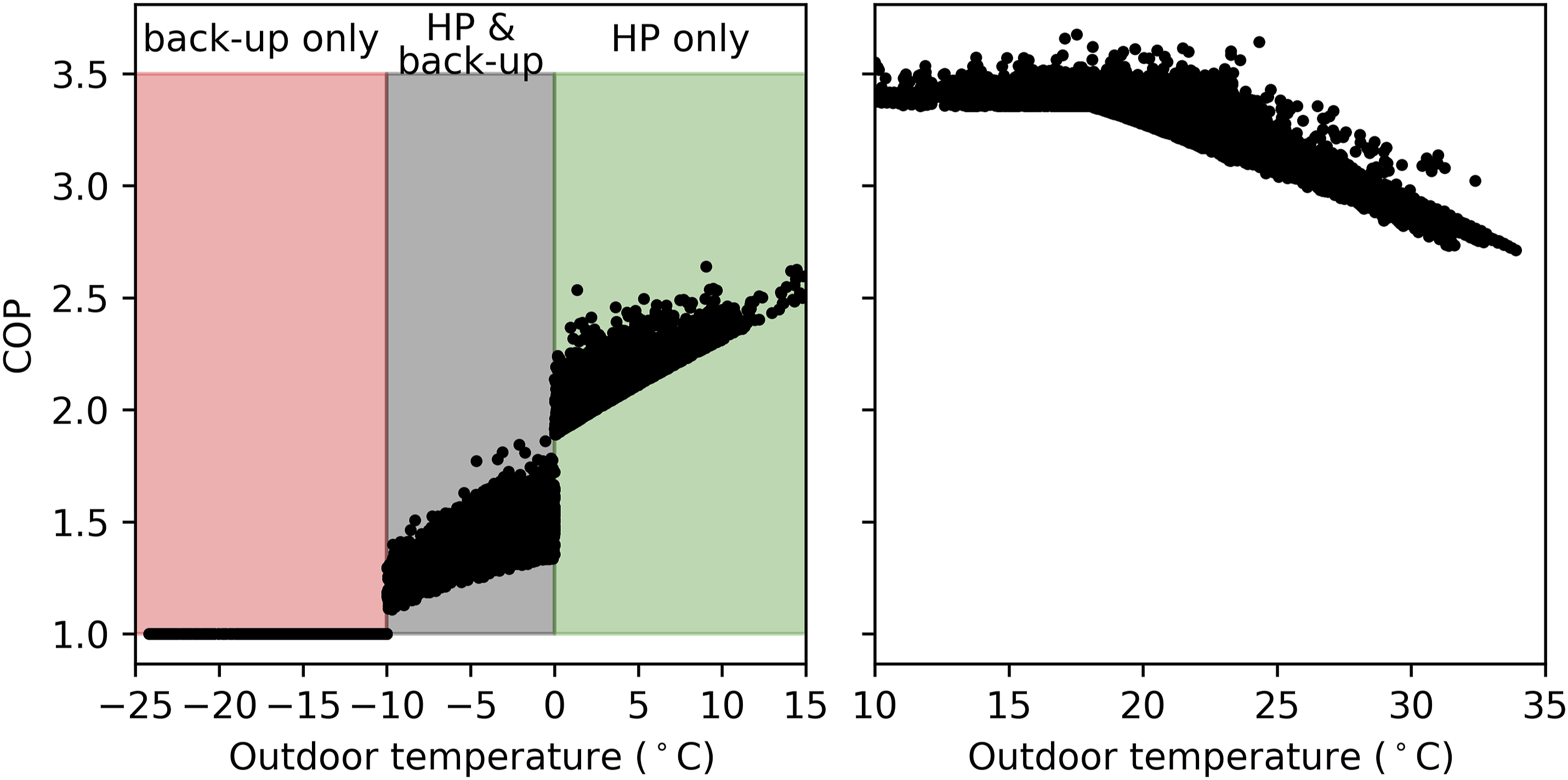
A BPS model representing a 458 m² one-storey small commercial building in Toronto, Canada is built in EnergyPlus v23.1. The floor height of the building is 3.5 m and the average window-to-wall ratio (WWR) is 12%; Figure 1 presents the floor plan of the building indicating the geometry and the breakdown of WWR on each orientation. The building is comprised of three thermal zones: a 175 m² lobby, 211 m² for offices, and a 72 m² electrical room. Each zone is served by a dedicated all-electric air-to-air heat pump. The gross-rated coefficients of performance (COP) of the heat pump for heating and cooling are assumed to be 2.75 and 3.0, respectively, with supplemental electric resistance heating for low-temperature operations. As shown in Table 1, the heat pumps are assumed to be available at outdoor temperatures higher than −10°C and the supplemental electric backup heating is assumed available at outdoor temperatures lower than 0°C. This led to the three distinct COP regimes shown in Figure 2.

Figure 1.

Floor plan of the building.

Table 1.

Model parameters and definitions for envelope, HVAC sizing, and occupants’ temperature preference scenarios.

Envelope	Windows	U_window 1.5 W/°C-m² (high performing envelope)
		U_window 2.0 W/°C-m² (average performing envelope)
		U_window 2.5 W/°C-m² (poor performing envelope)
		SHGC 0.39
	Opaque exterior	R_opaque 6°C-m²/W (high performing envelope)
		R_opaque 4°C-m²/W (average performing envelope)
		R_opaque 2°C-m²/W (poor performing envelope)
	Air permeance (normalized by above-grade exterior surface area)	0.15 L/s-m² (high performing envelope)
		0.25 L/s-m² (average performing envelope)
		0.35 L/s-m² (poor performing envelope)
HVAC	Setpoints	21°C-24°C (7 a.m. - 5 p.m., Mon to Sat)
	Setpoints	18°C-27°C (Otherwise)
	Outdoor air	2.5 L/s-person +0.3 L/s-m² (7 a.m. - 5 p.m. - Mon to Sat)
	Outdoor air	Differential dry-bulb economizer
	Heating	150 W/m² ASHP +80 W/m² electric back-up (over-sized heating)
		104 W/m² ASHP +80 W/m² electric back-up (normal-sized heating)
		58 W/m² ASHP +80 W/m² electric back-up (under-sized heating)
		ASHP minimum availability −10°C
		Back-up maximum availability 0°C
	Cooling	61 W/m² ASHP (over-sized cooling)
		49 W/m² ASHP (normal-sized cooling)
		37 W/m² ASHP (under-sized cooling)
	Fans	Always On
		Office RTU: 1.1 m³/s
		Lobby RTU: 1.1 m³/s
		Electrical RTU: 1.1 m³/s
Occupants	Occupancy	17 occupants (8 a.m. - 5 p.m. - Mon to Sat)
	Temperature preferences	21°C-25°C (Sensitive & warm preferring occupant scenario) 20°C-26°C (Tolerant & warm preferring occupant scenario) 20°C-24°C (Sensitive & cold preferring occupant scenario) 19°C-25°C (Tolerant & cold preferring occupant scenario)
	Lighting & plug loads	8 W/m² lighting (NECB lighting schedule)
	Lighting & plug loads	15 W/m² plug loads (NECB equipment schedule)

Figure 2.

Heating and cooling COP of the ASHP system at different outdoor temperature ranges.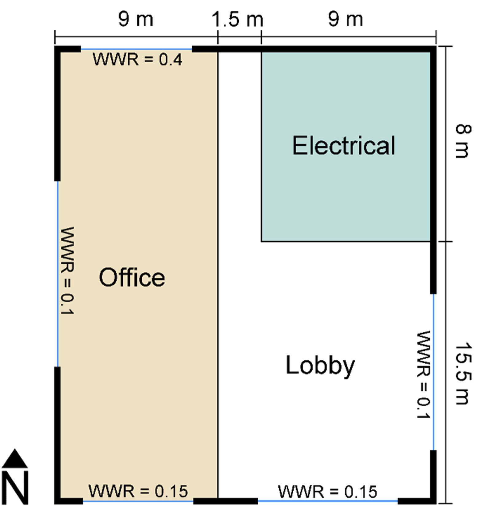

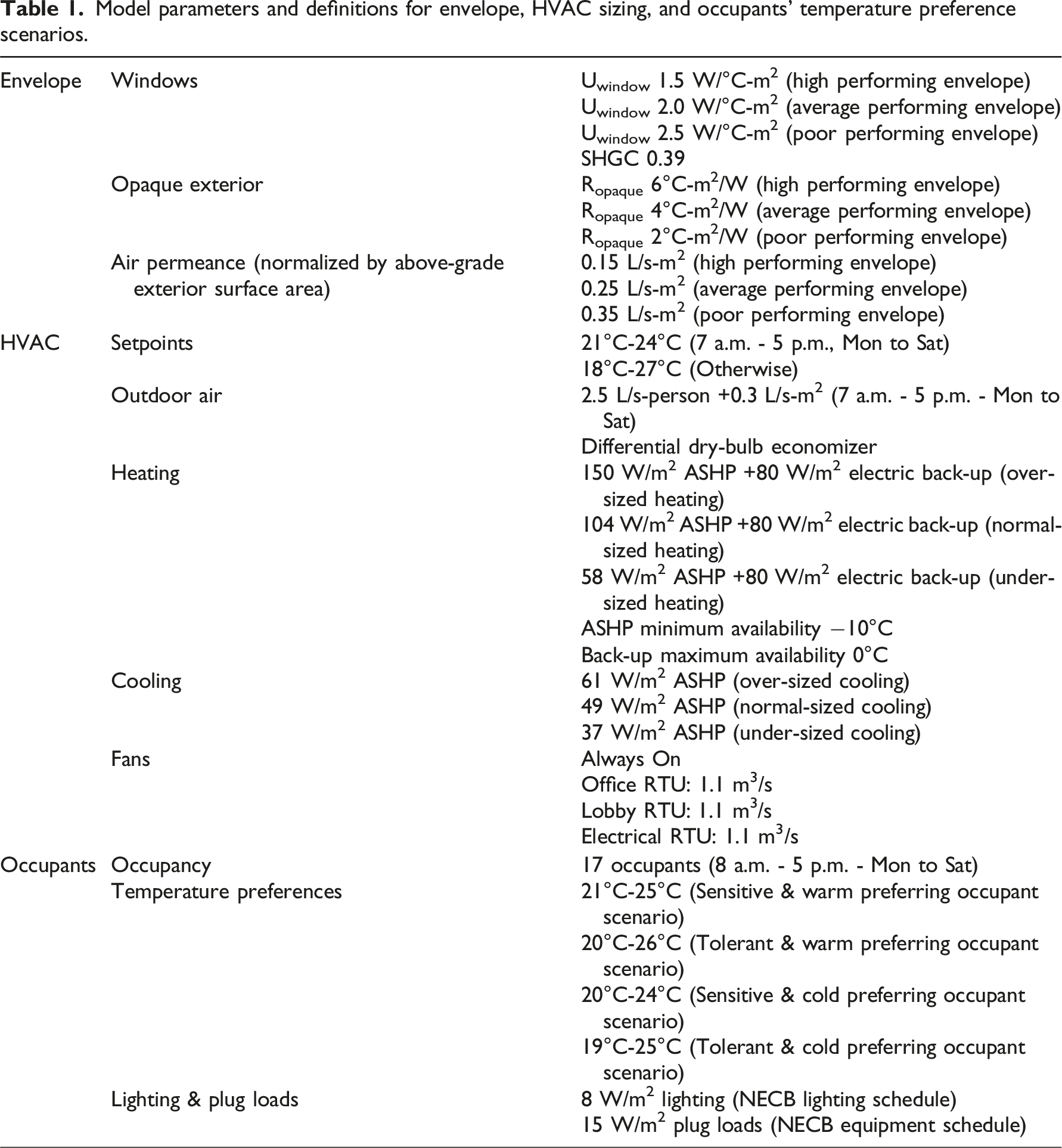
Each unit is coupled with a mixed-air single-zone air handler that uses a differential dry-bulb temperature-based economizer and is not equipped with any heat recovery capabilities. Up to 1.1 m³/s of supply air, comprised of a mixture of recirculated and outdoor air, is moved by each unit at a constant supply air pressure of 600 Pa and a supply air temperature (SAT) of 12.8°C in the cooling mode and 50°C in the heating mode. Canadian Weather Year for Energy Calculation (CWEC) data for Toronto is used for the year-long simulations³¹; the simulations are performed using 15-min timesteps. The heating and cooling temperature setpoints are 21°C and 24°C, respectively, during operating hours between 7 a.m. and 5 p.m. on weekdays and on Saturdays. Outside the operating hours, heating and cooling temperature setpoints are 18°C and 27°C, respectively. During operating hours, ventilation is set to 180 L/s on the basis of 2.5 L/s-person for a design occupancy of 17 persons and 0.3 L/s-m² per floor area. Note that the geometry of the building, thermal zones, and occupancy characteristics are based on a real small commercial building in Toronto, Canada. However, our analysis did not use the natural gas-based heating system of the actual building. Given the study’s focus on electrification and DLCs for HVAC systems, the emulator model was assembled with three air-source heat pumps (ASHP) serving the three thermal zones.

On average, each occupant, when present, is assumed to emit 125 W (i.e., light office work). Plug-in equipment and lighting loads are assumed to be 15 W/m² and 8 W/m², respectively, based on Bennett and O’Brien.³² National Energy Code for Buildings (NECB) schedule A was used for occupant, lighting, and equipment schedules.³³ Typical of North American small commercial building construction, the walls and the roof are defined with lightweight materials with negligible thermal mass – that is, steel-framed wall and roof with cavity and rigid insulation. The floor is defined with 20-cm thick concrete, which accounted for most of the thermal mass of the building enclosure. The concrete floor surface was assumed exposed to the indoor air and there was no insulative finishings like carpeting, vinyl flooring, etc. This assumption likely enhanced a DLC algorithm’s ability to store heat in the fabric during the preheating/precooling cycles. In addition, Hendron and Engebrecht³⁴ recommends assuming an internal mass of the furniture and contents as 39 kg/m². Given a 3.5 m column of air and density of indoor air of 1.2 kg/m³, the internal mass of the furniture and contents are accounted for with an indoor air capacitance multiplier of 9.3. Notably, these thermal mass-related assumptions play an important role in the temperature response during setpoint transition instances. While each building’s internal thermal mass amount and its distribution are expected to be somewhat different, the goal of this model was to have an emulator with plausible assumptions, which serves as a testbed for the assessment of the DLC algorithms.

As illustrated in Figure 3 36 variants of the base model are created representing three levels of envelope performance, three levels of HVAC sizing, and four different occupant temperature preference scenarios (3 × 3 × 4 = 36). Table 1 provides details regarding these scenarios. The envelope performance levels were taken from Ref.²⁷ where the average performance level corresponds to a NECB³³ compliant building for the local climate zone. Envelope scenarios poor and high correspond to thermal transmittance levels significantly higher and lower than the code-minimum envelope, respectively. The average HVAC sizing scenario was based on the actual building’s HVAC system information (i.e., nameplate thermal energy output capacity of the existing heating and cooling equipment). The under- and over-sized scenarios were generated by decreasing and increasing the heating and cooling capacities indicated in the average HVAC sizing scenario by 25%, respectively. Note that HVAC scenarios were created by varying the air-source heat pumps’ gross rated total heating and cooling capacities; all other HVAC-related model parameters (e.g., airflow rate, differential air pressure across the supply fan, supply air temperatures) were kept constant. Occupant preference scenarios represent four different plausible thresholds for thermostat override levels. They are inspired by Elehwany, et al.³⁵ Two of them represent occupants that accept up to a ±3°C variation from their preferred temperature of 22°C or 23°C (which we refer to as tolerant occupants), and the other two represent occupants that accept up to a ±2°C variation from their preferred temperature of 22°C or 23°C (which we refer to as sensitive occupants). Variations in temperature preferences are typical, and they can be explained with variations in the metabolic rates, clothing insulation levels, and other non-temperature physical variables (e.g., air speed, surface temperatures, etc.). Note that EnergyPlus was selected as the engine for our emulator model because it is a research-grade open-source tool, widely used in BPS research and practice, and it offers the flexibility of testing advanced control algorithms via its Python application programming interface (API).

Figure 3.

Envelope, HVAC sizing, and occupant preference scenarios.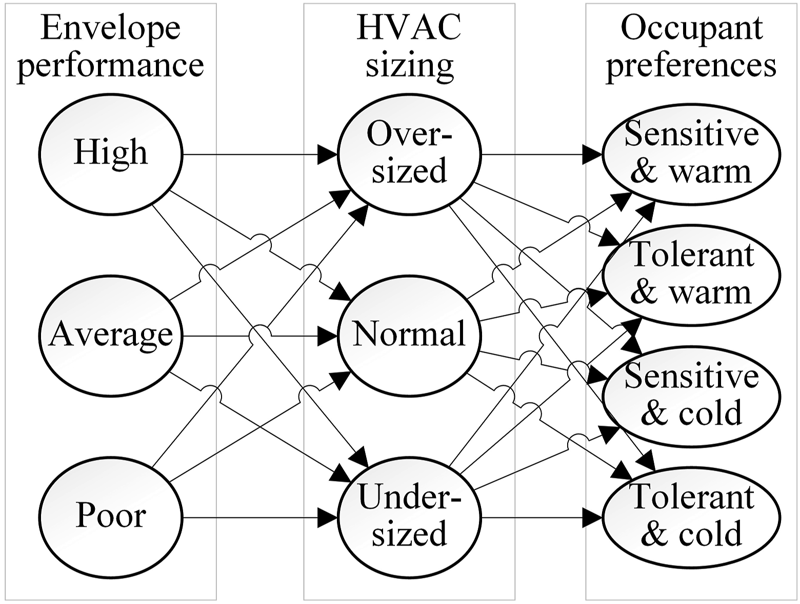

TOU pricing and DLC parameters

The TOU rates applicable to small commercial buildings in Ontario for 2023 are shown in Figure 4. In the heating season (i.e., November through April inclusive) on weekdays, there are two on-peak periods: in the morning between 7 a.m. and 11 a.m. & in the evening between 5 p.m. and 7 p.m. Because the default settings for the evening peak period already apply a setback temperature of 18°C in the heating season, a DLC intervention is relevant for the morning peak periods only. As shown in Figure 4, the heating season DLC sequence is defined with three parameters: preheating magnitude (ΔT_ph), preheating duration (Δt_ph), and setback magnitude (ΔT_sb).

Figure 4.

TOU rates and DLC sequence shape and parameters for (a) Winter (November to April) (b) Summer (May to October). The acronyms HSP and CSP stand for the heating and cooling temperature setpoints, respectively.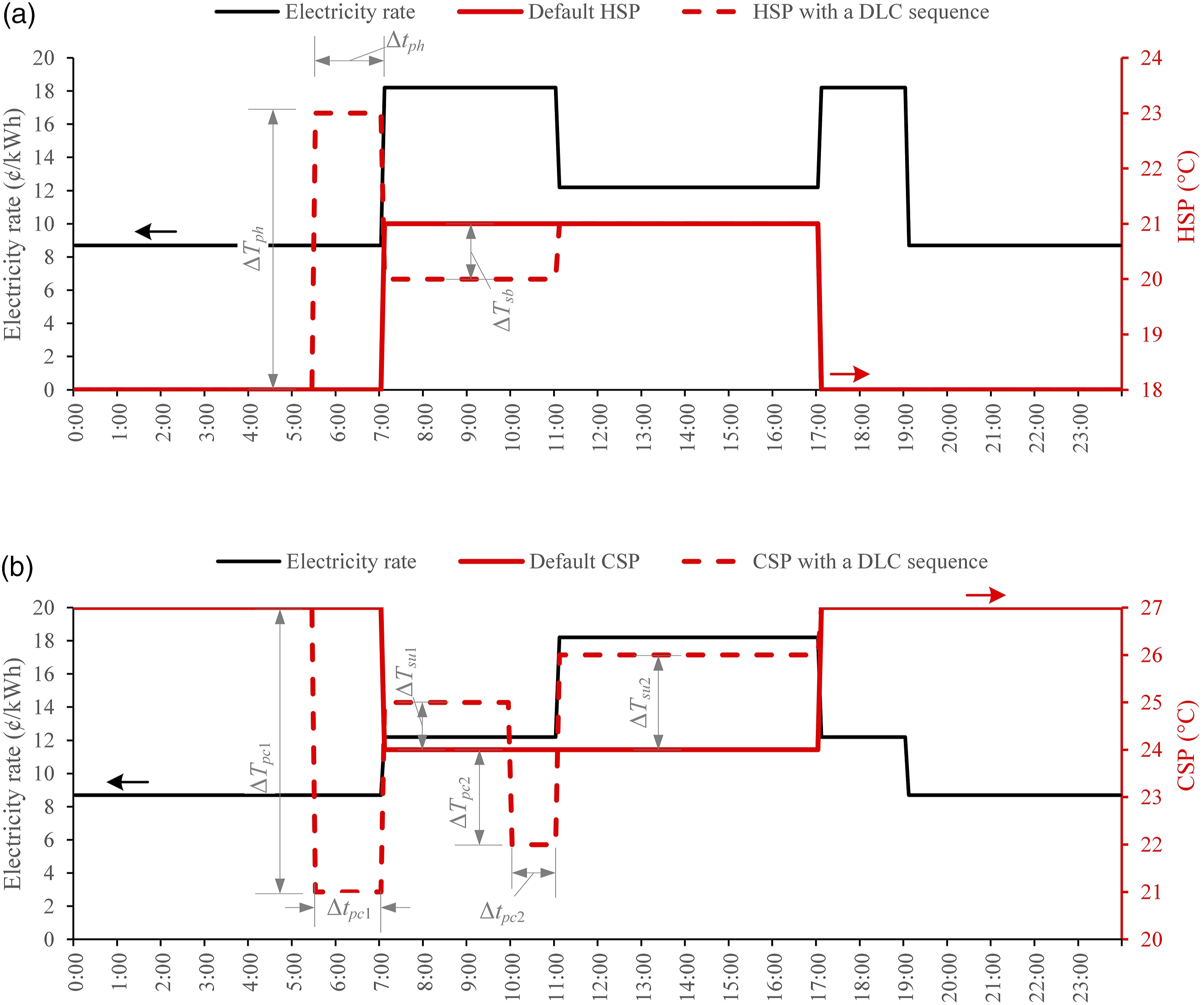

In the cooling season (i.e., May through October inclusive) on weekdays, there are two instances where the cost of electricity increases during operating hours. A transition from off-peak to mid-peak rates takes place at 7 a.m. and a transition from mid-peak to on-peak rates take place at 11 a.m. Thus, the cooling season DLC sequence is defined with six parameters: early morning precooling magnitude (ΔT_pc1), early morning precooling duration (Δt_pc1), early morning setup magnitude (ΔT_su1), late morning precooling magnitude (ΔT_pc2), late morning precooling duration (Δt_pc2), and late morning/afternoon setup magnitude (ΔT_su2).

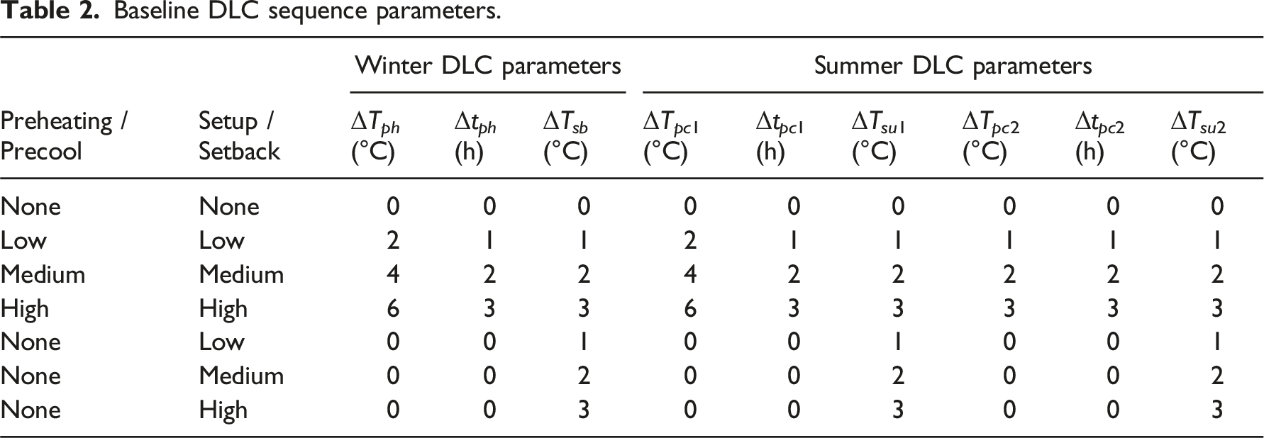
Baseline DLC sequences

The 36 variants of the BPS model introduced in Figure 3 (3 envelope tiers × 3 HVAC sizing tiers × 4 occupant preferences) are simulated with seven baseline DLC sequences shown in Table 2. These baselines represent a no DLC version, three DLC sequences with preheating/precooling, and three DLC sequences without preheating/precooling. Two metrics are computed for each run case: the electricity cost for HVAC and the hours spent outside the preferred temperature ranges of each BPS model variant (indicated in Figure 3 and Table 1). The performance of the seven sequences is reported based on the distribution of the two metrics computed for the 36 BPS models. These results act as baseline performance levels that can be obtained through generic one-fits-for-all DLC sequences applied across a portfolio of buildings, disregarding their HVAC and envelope characteristics and occupant preferences.

Table 2.

Baseline DLC sequence parameters.

Preheating / Precool	Setup / Setback	Winter DLC parameters			Summer DLC parameters
Preheating / Precool	Setup / Setback	ΔT_ph (°C)	Δt_ph (h)	ΔT_sb (°C)	ΔT_pc1 (°C)	Δt_pc1 (h)	ΔT_su1 (°C)	ΔT_pc2 (°C)	Δt_pc2 (h)	ΔT_su2 (°C)
None	None	0	0	0	0	0	0	0	0	0
Low	Low	2	1	1	2	1	1	1	1	1
Medium	Medium	4	2	2	4	2	2	2	2	2
High	High	6	3	3	6	3	3	3	3	3
None	Low	0	0	1	0	0	1	0	0	1
None	Medium	0	0	2	0	0	2	0	0	2
None	High	0	0	3	0	0	3	0	0	3

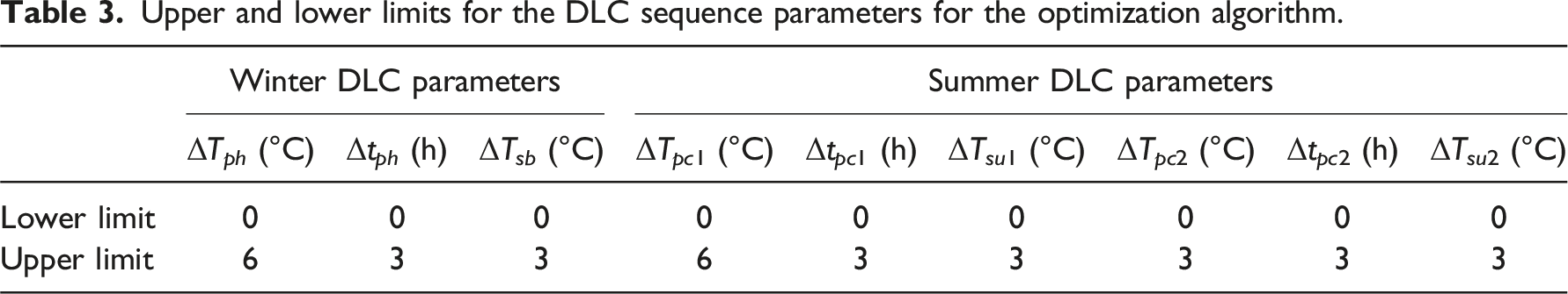
Optimization algorithm for DLC sequence derivation

A metaheuristic search algorithm, differential evolution method,³⁶ was employed to estimate the nine DLC sequence parameters minimizing the following cost function:

f (x) = C_{e l e c} \cdot (1 + {(f_{d i s c o m f o r t})}^{2})

(1)

where x is an array containing the DLC sequence parameters, C_elec ($) is the annual electricity cost for HVAC, and f_discomfort is the percentage of time spent outside low and high limits of comfort defined in Table 1. Notably, the cost reduces to the cost of electricity when f_discomfort is zero. The parenthetical discomfort term implies that the cost of electricity is inflated by 1% when f_discomfort is 1%, by 9% when f_discomfort is 3%, and by 100% when f_discomfort is 10%. Simply put, the quadratically increasing comfort-based penalty is designed to minimize the risk of comfort violations. The differential evolution method was used as implemented in Python’s scipy package v1.12.0.³⁷ The population size and number of generations were set as 72 and six, respectively. These hyperparameters were selected by iteratively increasing the population size and number of generations with one of the 36 variant models. This process was intended to balance the runtime and the repeatability of the results. The simulations were carried out by using the EnergyPlus Python API. The nine DLC parameters were then searched within the upper and lower bounds defined in Table 3.

Table 3.

Upper and lower limits for the DLC sequence parameters for the optimization algorithm.

	Winter DLC parameters			Summer DLC parameters
	ΔT_ph (°C)	Δt_ph (h)	ΔT_sb (°C)	ΔT_pc1 (°C)	Δt_pc1 (h)	ΔT_su1 (°C)	ΔT_pc2 (°C)	Δt_pc2 (h)	ΔT_su2 (°C)
Lower limit	0	0	0	0	0	0	0	0	0
Upper limit	6	3	3	6	3	3	3	3	3

Results and discussion

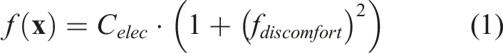
Figure 5 presents the evolution of the objective (i.e., cost defined in Equation (1)), the electricity cost, and the f_discomfort term in multiple generations for the variant with high-performing envelope, oversized HVAC, and tolerant & warmer temperature preferring occupant scenarios. Each boxplot is an outcome of 72 simulations with various DLC sequence parameters. The results indicate that the median objective value of each generation iteratively reduces for the first five generations through resampling of high-performing DLC sequences. Similarly, the median electricity cost and f_discomfort values slowly improved across multiple generations. Because of mutation and crossover, the diversity among the 72 members was largely retained after six generations. This diversity was essential to minimize the risk of getting stuck in a local minimum. The evolution patterns observed with the other variants were similar – that is, the median of the objective stopped improving in either the fourth or fifth generations. Thus, similar graphs were not included to avoid repetition.

Figure 5.

Evolution of the objective function, annual electricity cost and fraction of times spent outside low and high limits of comfort for the variant with high-performing envelope, oversized HVAC, and tolerant & warmer temperatures preferring occupants.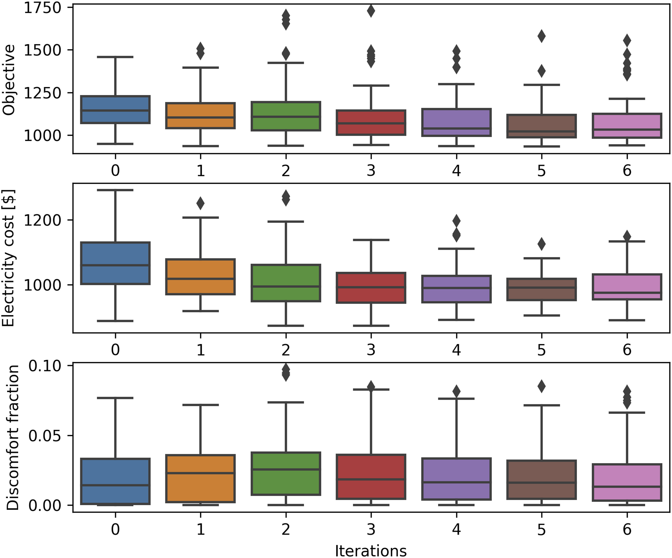

Figure 6 presents the pairwise relationship between the annual electricity cost and the f_discomfort values for 504 (72 simulations/generation × 7 generations) different DLC sequences for the same variant. The results indicate that close to the x-axis there is great variation in the performance where DLC sequences can offer electricity cost savings with little to no f_discomfort.

Figure 6.

Pairwise relationship between the annual cost and fraction of times spent outside low and high temperature limits during the optimization process for the variant with high-performing envelope, oversized HVAC, and tolerant & warmer temperatures preferring occupants.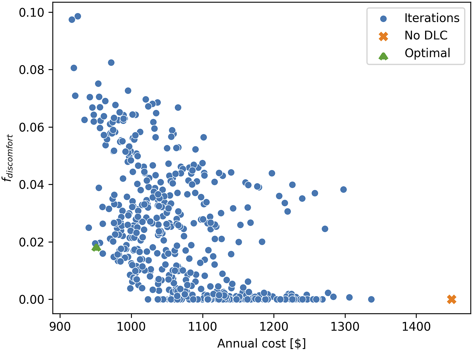

The optimal DLC parameters for each variant are listed in Table 4. The results indicate the mean and the standard deviation of optimal preheating magnitude ΔT_ph were 3.7°C and 1.3°C, respectively. The optimal ΔT_ph value for the variants with the high-performing envelope scenario was on average 1.6°C less than those with the poor-performing envelope scenario. This can be attributed to the fact that variants with the high-performing envelope scenario need to store much less thermal energy during off-peak hours to eliminate their on-peak electricity use for heating. The average and standard deviation of the optimal preheating duration Δt_ph were 1 h and 0.5 h, respectively. The optimal preheating duration with the oversized HVAC scenario was on average 0.4 h shorter than with the undersized HVAC scenario. The optimal setback magnitude ΔT_sb was typically at the lower limit of the preferred indoor temperatures (i.e., 1°C for tolerant and warm, 0°C for sensitive and warm, 1°C for sensitive and cold, 2°C for tolerant and cold) for the variants with the poor envelope scenario. For those with average and high-performing envelope scenarios, the ΔT_sb sometimes exceeded the comfort limits. This is likely because of their higher thermal autonomy. Consequently, the variants with average and high-performing envelopes, despite these larger setback magnitudes ΔT_sb, did not experience frequent violations of the preferred temperature limits thanks to their thermal autonomy.

Table 4.

The optimal DLC parameters for each variant. µ and σ stand for mean and standard deviation. The labels he, ae, and pe represent high-, average-, and poor-performing envelope, respectively. The labels ns, us, and os represent normal-, under-, and over-sized HVAC, respectively. The labels one to four represent occupant temperature preference scenarios: tolerant & warm, sensitive & warm, sensitive & cold, and tolerant & cold, respectively. Refer to Table 1 for definitions of these attributes used in assembling the 36 scenarios.

Variant	ΔT_ph (°C)	Δt_ph (h)	ΔT_sb (°C)	ΔT_pc1 (°C)	Δt_pc1 (h)	ΔT_su1 (°C)	ΔT_pc2 (°C)	Δt_pc2 (h)	ΔT_su2 (°C)
he/ns/1	2.4	0.6	2.6	3.8	0.7	1.6	2.5	0.2	2.0
ae/ns/1	4.8	0.7	1.0	1.3	1.4	2.0	2.6	0.2	2.0
pe/ns/1	4.5	0.8	1.1	3.5	0.2	1.6	0.9	2.3	1.8
he/us/1	2.9	0.6	2.4	3.2	0.1	1.9	1.6	0.2	2.1
ae/us/1	3.4	2.6	2.2	5.2	1.2	0.4	0.5	0.4	2.1
pe/us/1	3.3	1.3	0.9	4.6	1.6	2.3	0.4	2.1	2.0
he/os/1	3.2	1.3	2.4	3.3	1.4	2.3	2.1	0.2	2.0
ae/os/1	5.7	0.7	2.5	6.0	0.3	2.7	0.4	1.3	2.1
pe/os/1	5.6	0.5	1.0	2.1	1.3	1.3	1.1	0.1	1.9
he/ns/2	4.7	0.6	1.9	3.8	0.2	1.0	0.1	1.2	0.6
ae/ns/2	4.6	1.3	2.3	1.7	2.4	0.1	0.5	1.2	1.0
pe/ns/2	4.6	1.5	0.0	4.0	2.2	2.5	0.8	2.8	1.0
he/us/2	3.4	1.4	2.9	2.9	2.5	1.6	0.0	1.7	0.9
ae/us/2	5.2	1.3	1.7	3.5	0.9	0.7	0.2	0.5	0.7
pe/us/2	3.3	1.0	0.0	0.8	2.1	0.9	1.8	1.9	1.0
he/os/2	3.9	1.2	2.3	1.3	1.1	0.3	1.8	0.2	1.0
ae/os/2	5.7	0.7	2.5	3.1	0.8	1.5	0.4	2.2	0.7
pe/os/2	5.3	0.8	0.0	3.4	1.1	2.0	2.1	2.5	1.1
he/ns/3	2.7	1.0	1.0	0.3	1.6	0.9	1.6	2.8	0.1
ae/ns/3	4.7	1.8	3.0	1.6	2.3	1.7	2.1	1.9	0.0
pe/ns/3	4.7	0.8	1.0	4.1	0.8	0.1	0.3	2.0	0.0
he/us/3	2.6	1.4	2.3	3.2	0.5	0.3	0.1	2.5	0.0
ae/us/3	3.5	1.9	2.7	0.8	2.2	0.6	2.8	2.4	0.1
pe/us/3	3.5	1.6	0.9	1.4	0.4	0.3	1.6	2.4	0.0
he/os/3	3.4	1.7	2.4	4.6	0.6	0.7	1.4	0.6	0.1
ae/os/3	3.6	0.6	1.0	4.0	1.4	1.8	1.4	1.6	0.0
pe/os/3	2.0	1.3	0.6	4.6	0.9	1.2	0.9	2.7	0.0
he/ns/4	0.5	1.1	1.9	3.5	2.3	1.2	0.1	2.7	1.0
ae/ns/4	2.7	0.7	2.1	4.4	0.9	1.0	1.7	0.4	1.1
pe/ns/4	4.6	0.6	2.3	3.5	1.5	1.5	0.2	1.8	1.1
he/us/4	1.7	0.6	2.5	0.0	2.0	0.3	0.2	0.6	0.8
ae/us/4	3.4	0.8	2.0	1.5	2.5	0.3	0.5	1.6	1.1
pe/us/4	3.4	0.6	2.8	3.7	2.8	0.5	0.1	1.3	1.0
he/os/4	0.5	0.6	2.1	3.6	1.2	0.9	1.0	1.6	1.0
ae/os/4	2.6	0.3	2.7	2.8	0.5	2.8	0.0	2.9	1.1
pe/os/4	5.8	0.9	2.3	1.1	0.7	0.5	0.7	1.9	1.0
µ	3.7	1.0	1.8	3.0	1.3	1.2	1.0	1.5	1.0
σ	1.3	0.5	0.9	1.4	0.8	0.8	0.8	0.9	0.7

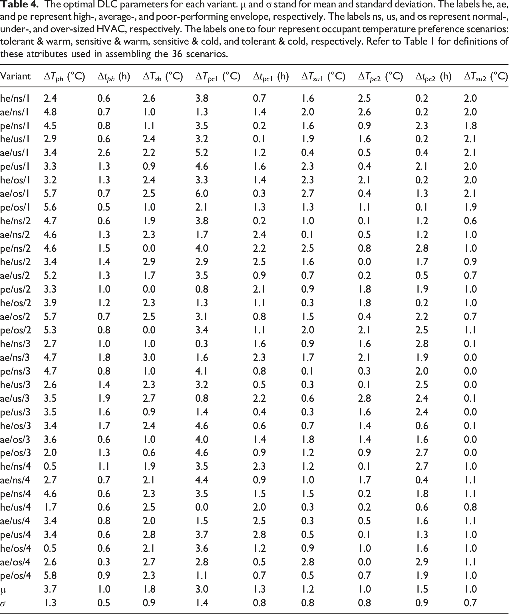
The mean and the standard deviation for the optimal morning precooling magnitude ΔT_pc1 were 3°C and 1.4°C, respectively. And the mean and the standard deviation for the optimal morning precooling duration Δt_pc1 were 1.3 h and 0.8 h, respectively. On average, the variants with the oversized HVAC scenario had an optimal ΔT_pc1 value 0.8°C greater and an optimal Δt_pc1 value 0.6 h shorter than those with the undersized HVAC scenario. Simply put, the variants with an oversized HVAC system could deliver the necessary precooling in a shorter period of time at a greater intensity. The optimal setup parameters ΔT_su1 and ΔT_su2 were typically confined by the upper limit of the preferred temperature ranges (i.e., 2°C for tolerant and warm, 1°C for sensitive and warm, 0°C for sensitive and cold, 1°C for tolerant and cold). However, a few of the variants with the undersized HVAC scenario ended up with smaller ΔT_su1 and ΔT_su2 values. This is likely because of the risk of frequent discomfort conditions due to longer recovery times with the undersized HVAC scenarios. The mean and the standard deviation for the optimal daytime precooling magnitude ΔT_pc2 were 1°C and 0.8°C, respectively. And the mean and the standard deviation for the optimal daytime precooling duration Δt_pc2 were 1.5 h and 0.9 h, respectively. On average, the optimal Δt_pc2 was 0.8 h longer with the poor envelope scenario than with the high-performing envelope scenario. The results, in general, highlight the significance of inter-variant diversity of the optimal DLC sequences and the need for personalized building-specific DLC sequences. Figure 7 provides a visualization of this diversity. Notably, the variants of this study are built upon the same archetype – for example, same orientation, WWR, occupancy, lighting, and plug-in equipment load intensities. In reality, the inter-building diversity of optimal DLC sequences would even be greater, if the variants were generated from different small commercial building archetypes.

Figure 7.

The optimal DLC sequences for heating setpoints (HSP) and cooling setpoints (CSP) for each variant and their mean.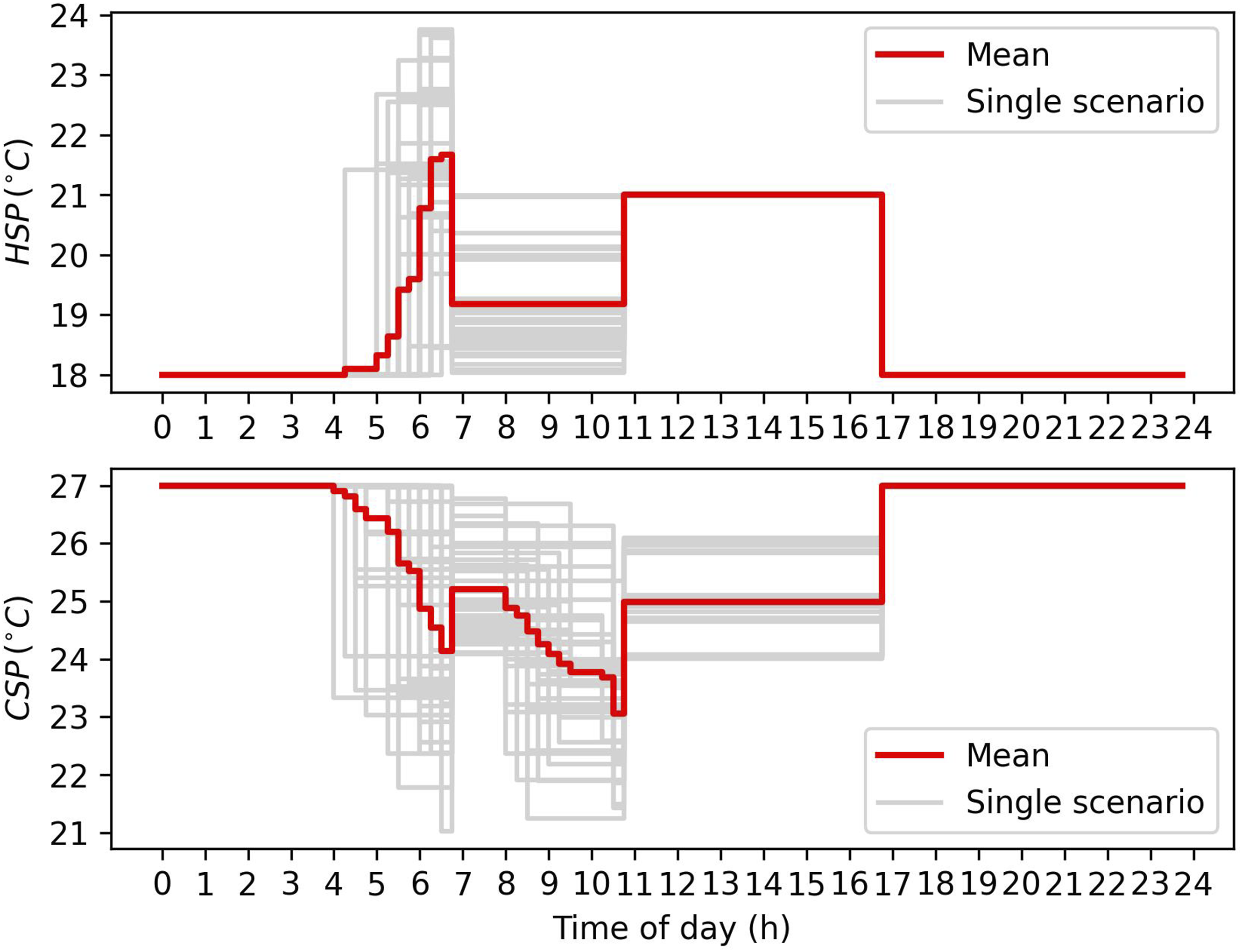

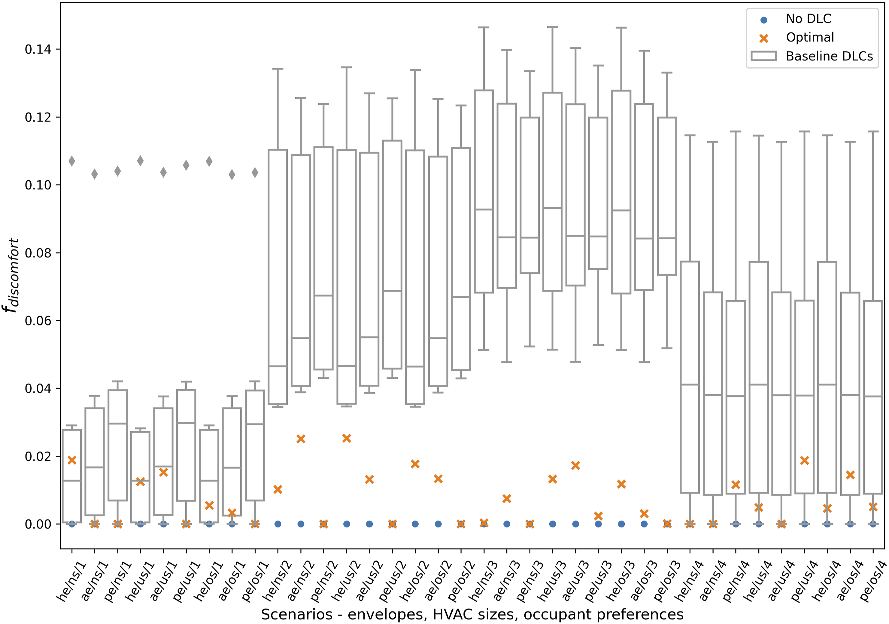
Figure 8 presents the annual electricity cost of the 36 variants with the optimal and baseline DLC sequences. The mean and standard deviation of the HVAC electricity cost savings with the optimal DLC sequences relative to the no DLC case were 20% and 7%, respectively. The average HVAC electricity cost savings were 28%, 20%, and 13% with the high-, average-, and poor-performing envelope scenarios, respectively. Despite these large variations in the percent cost savings, the absolute HVAC electricity cost savings were on average about $420 ($0.9 per m² floor area) for all three tiers of the envelope scenarios. The average cost savings potential was 24% and 17% with the tolerant and sensitive occupant scenarios, respectively. This corresponds to an average of $490 of savings with the tolerant occupant scenarios and $340 of savings with the sensitive occupant scenarios. The electricity cost savings potential was on average $75 greater with an oversized HVAC system in contrast to an undersized HVAC system. This can be explained by an increased capacity to deliver intended heating/cooling energy during preheating/precooling periods. At least some of the baseline DLC sequences were able to achieve electricity cost savings comparable to the sequence estimated via optimization. However, the baseline DLC sequences caused many hours spent outside the preferred temperature ranges (see Figure 9). The optimization process maintained the f_discomfort metric consistently under 3%. These findings highlight that the one-size-fits-all approach to DLC with generic sequences causes either discomfort or suboptimal electricity cost savings.

Figure 8.

The annual electricity cost with the six generic DLC and no DLC baselines listed in Table 2, and the optimal DLC sequences for the 36 variants. The labels he, ae, and pe represent high-, average-, and poor-performing envelope, respectively. The labels ns, us, and os represent normal-, under-, and over-sized HVAC, respectively. The labels one to four represent occupant temperature preference scenarios: tolerant & warm, sensitive & warm, sensitive & cold, and tolerant & cold, respectively. Refer to Table 1 for definitions of these attributes used in assembling the 36 scenarios.

Figure 9.

The fraction of time spent outside preferred temperature bounds with the six generic DLC and no DLC baselines listed in Table 2, and the optimal DLC sequences for the 36 variants. The labels he, ae, and pe represent high-, average-, and poor-performing envelope, respectively. The labels ns, us, and os represent normal-, under-, and over-sized HVAC, respectively. The labels one to four represent occupant temperature preference scenarios: sensitive & warm, tolerant & warm, sensitive & cold, and tolerant & cold, respectively. Refer to Table 1 for definitions of these attributes used in assembling the 36 scenarios.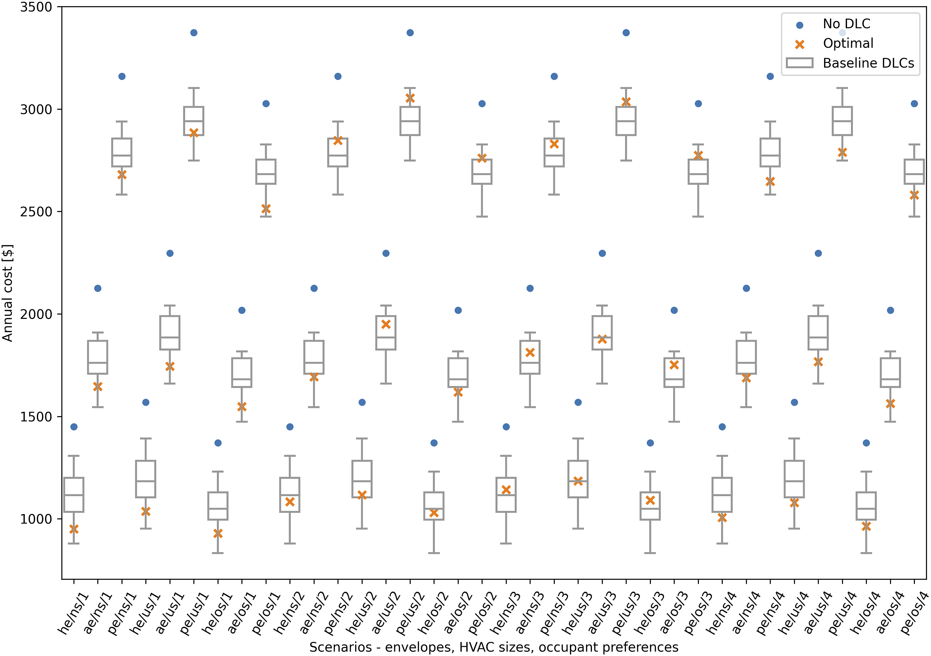

Unresolved issues

This paper demonstrated that DLC sequences that minimize the electricity cost while maintaining the temperatures within a user’s preferred temperature range are unique for each building. Optimal DLC sequences were derived for variants of a small commercial building archetype. These sequences can be implemented in programmable thermostats controlling electric HVAC systems in similar buildings. Choosing the right sequence requires a rough estimate of the envelope and HVAC-sizing characteristics. In some cases, these characteristics can be inferred from the building age (i.e., applicable code requirements of the vintage), retrofit history, and nameplate data regarding the HVAC system capacity. Alternatively, surrogate model- or inverse model-based envelope characterization approaches^38–40 can be applied to gain insights into these attributes.

In this study, only a single set of winter and summer DLC sequences was derived. In reality, it is logical that the preheating/precooling needs during the shoulder season months differ from those during the core heating and cooling season months. Future work should derive different DLC sequences for the shoulder seasons. The same BPS-based global optimization approach can be employed to search for four sets of DLC sequences (Winter, Spring, Summer, Fall), instead of the two searched in this paper.

The estimation of optimal DLC sequences was done through a simulation-based investigation. Future work should implement them in actual small commercial buildings to assess occupant comfort, behaviour, and perception of DLC.

The DLC sequences studied in this paper incorporated both preconditioning and setup/setback. It is likely that some facility managers may have contractual constraints preventing them from applying temperature setups/setbacks. Future work should investigate the savings potential merely through preheating/precooling.

The DLC sequences employed in this study had instantaneous setpoint increases/decreases at transitions to/from preconditioning and setup/setback periods. Such rapid transitions in the Winter may cause inefficient electric or natural gas auxiliary heating systems to engage and cause abrupt peaks, which may pose risks at the building electric panel level or collectively at the substation level. During the real-world implementation, rebound mitigation sequences shall be incorporated such that setpoints transition incrementally over a reasonable period of time (e.g., 30-min).⁴¹

This study was conducted in a jurisdiction where the on-peak to off-peak electricity cost ratio is about two. The cost of over-preconditioning is non-negligible. At higher on-peak to off-peak rate ratios, as preconditioning becomes cheaper, the tendency of an optimization algorithm would be to increase the preheating/precooling magnitudes and durations. At lower on-peak to off-peak rate ratios, the tendency would be to reduce preheating/precooling magnitudes and durations, as over-preconditioning would become a more expensive mistake. Future work should investigate different peak pricing scenarios. In addition, the scope of our findings is limited to small commercial buildings served by air-source heat pump systems. The findings should not be directly extrapolated to other building typologies with different HVAC configurations.

Conclusion and future work

In this paper, a metaheuristic search algorithm was employed to derive a personalized DLC sequence for each building typology separately. The algorithm estimated a unique DLC sequence that minimizes the electricity cost, and the time spent outside a preferred temperature range for each building.

The optimization was formulated by using 36 variants of an EnergyPlus model representing a standalone small commercial building in Toronto, Canada. These variants were generated by systematically altering the model’s envelope properties, HVAC system’s capacity, and occupants’ temperature preferences. The optimization algorithm was implemented to interact with the model via EnergyPlus’ Python API. The optimal DLC sequences were compared with six generic baseline DLC sequences. Of them, three apply preconditioning and setup/setback at varying intensities and durations. The rest only apply setup/setback at varying intensities and durations.

The results demonstrated the inter-building diversity in optimal DLC sequences (recall Research Question one in Subsection 1.3). For example, the mean and the standard deviation of optimal preheating magnitude were 3.7°C and 1.3°C, respectively. The mean and the standard deviation for the optimal precooling magnitude were 3°C and 1.4°C, respectively. The standard deviation (indicative of the inter-building diversity) of the DLC sequences could largely be explained by the differences in the building envelope, HVAC sizing, and occupants’ temperature preferences. For example, the optimal preheating magnitude for the variants with the high-performing envelope scenario was on average 1.6°C less than those with the poor-performing envelope scenario. The variants with the oversized HVAC scenario had an optimal precooling magnitude 0.8°C greater and an optimal precooling duration 0.6 h shorter than those with the undersized HVAC scenario. The HVAC electricity cost savings with the optimal DLC sequences also exhibit significant variation. While the mean electricity cost saving relative to the no DLC case was 20%, the standard deviation amongst the variants was 7%. None of the baseline DLC sequences could attain similar electricity cost savings without causing excessive discomfort (recall Research Question 2 in Subsection 1.3). The optimal DLC sequences could keep the time spent outside the preferred temperature ranges under 3% for all variants. Future work should investigate the effect of optimizing for a different DLC sequence for the shoulder season months in addition to the core heating and cooling seasons.

Footnotes

Declaration of conflicting interests

The author(s) declared no potential conflicts of interest with respect to the research, authorship, and/or publication of this article.

Funding

The author(s) disclosed receipt of the following financial support for the research, authorship, and/or publication of this article: This research is supported by a research contract with the National Research Council Canada (Contract number 1011603).

ORCID iDs

Hussein Elehwany

Brodie W. Hobson

Appendix

Table A1.

List of symbols.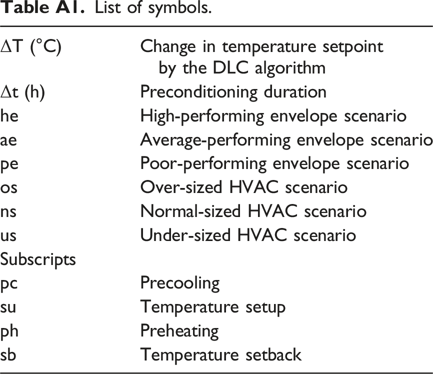

ΔT (°C)	Change in temperature setpoint by the DLC algorithm
Δt (h)	Preconditioning duration
he	High-performing envelope scenario
ae	Average-performing envelope scenario
pe	Poor-performing envelope scenario
os	Over-sized HVAC scenario
ns	Normal-sized HVAC scenario
us	Under-sized HVAC scenario
Subscripts
pc	Precooling
su	Temperature setup
ph	Preheating
sb	Temperature setback

References

Deason

Wei

Leventis

, et al. Electrification of buildings and industry in the United States: drivers, barriers, prospects, and policy approaches. 2018. Available from: https://www.osti.gov/servlets/purl/1430688/

Afroz

Goldsworthy

White

. Energy flexibility of commercial buildings for demand response applications in Australia. Energy Build 2023; 300: 113533.

Piette

Kiliccote

Dudley

. Field demonstration of automated demand response for both winter and summer events in large buildings in the Pacific Northwest. Energy Efficiency 2013; 6(4): 671–684.

De Chalendar

McMahon

Fuentes Valenzuela

, et al. Unlocking demand response in commercial buildings: empirical response of commercial buildings to daily cooling set point adjustments. Energy Build 2023; 278: 112599.

Chen

, et al. Quantification of electricity flexibility in demand response: office building case study. Energy 2019; 188: 116054.

Markus

Hobson

Bursill

, et al. Load reduction potential of generic automated demand-response sequences with coincident peak pricing. 2024 ASHRAE Winter Conference. ASHRAE Transactions, 2024, pp. 552–561. Available from: https://store.accuristech.com/ashrae/standards/ch-24-c066-load-reduction-potential-of-generic-automated-demand-response-sequences-with-coincident-peak-pricing?product_id=2904916

Tina

Aneli

Gagliano

. Technical and economic analysis of the provision of ancillary services through the flexibility of HVAC system in shopping centers. Energy 2022; 258: 124860.

Fournier

Leduc

Nadrault

. Winter demand response using baseboard heaters: achieving substantial demand reduction without sacrificing comfort. In: Proceedings of ACEEE Summer Study on. Energy Efficiency in Buildings, 2016, pp. 1–12.

Pardasani

Veitch

, et al. Demand control of baseboard heaters using connected thermostats: lessons learned from a 567-home pilot study. Build Eng 2020; 126: 12–20.

10.

ASHRAE . Standard 90.1. American Society of Heating, Refrigerating, and Air-Conditioning. 2022.

11.

ASHRAE . Standard 55: thermal environmental conditions for human occupancy. American Society of Heating, Refrigerating, and Air-Conditioning 2020.

12.

Granderson

Fernandes

Crowe

, et al. Accuracy of hourly energy predictions for demand flexibility applications. Energy Build 2023; 295: 113297.

13.

Johra

De Andrade Pereira

, et al. Data-driven key performance indicators and datasets for building energy flexibility: a review and perspectives. Appl Energy 2023; 343: 121217.

14.

Huang

Katipamula

Lutes

. Experimental investigation on thermal inertia characterization of commercial buildings for demand response. Energy Build 2021; 252: 111384.

15.

Sarran

Gunay

O’Brien

, et al. A data-driven study of thermostat overrides during demand response events. Energy Policy 2021; 153(April): 112290.

16.

Khorasani Zadeh

Ouf

Gunay

, et al. Development of prediction models for thermostat override behavior in direct load control events. Energy Build 2023; 301: 113707.

17.

Gehbauer

Lee

Wang

. An evaluation of the demand response potential of integrated dynamic window and HVAC systems. Energy Build 2023; 298: 113481.

18.

Deng

Wang

Dong

. Quantum computing for future real-time building HVAC controls. Appl Energy 2023; 334: 120621.

19.

Chen

Cao

Pouramini

. Energy cost and consumption reduction of an office building by Chaotic Satin Bowerbird Optimization Algorithm with model predictive control and artificial neural network: a case study. Energy 2023; 270: 126874.

20.

Reynolds

Rezgui

Kwan

, et al. A zone-level, building energy optimisation combining an artificial neural network, a genetic algorithm, and model predictive control. Energy 2018; 151: 729–739.

21.

Afram

Janabi-Sharifi

. Supervisory model predictive controller (MPC) for residential HVAC systems: implementation and experimentation on archetype sustainable house in Toronto. Energy Build 2017; 154: 268–282.

22.

Meimand

Jazizadeh

. A personal touch to demand response: an occupant-centric control strategy for HVAC systems using personalized comfort models. Energy Build 2024; 303: 113769.

23.

Soudari

Srinivasan

Balasubramanian

, et al. Learning based personalized energy management systems for residential buildings. Energy Build 2016; 127: 953–968.

24.

Kamal

Moloney

Wickramaratne

, et al. Strategic control and cost optimization of thermal energy storage in buildings using EnergyPlus. Appl Energy 2019; 246: 77–90.

25.

Henze

Kircher

Braun

. Why has advanced commercial HVAC control not yet achieved its promise? Journal of Building Performance Simulation 2024; 18: 217–228.

26.

Kim

Braun

. Development, implementation and performance of a model predictive controller for packaged air conditioners in small and medium-sized commercial building applications. Energy Build 2018; 178: 49–60.

27.

Gunay

Newsham

Ashouri

, et al. Deriving sequences of operation for air handling units through building performance optimization. Journal of Building Performance Simulation 2020; 13(5): 501–515.

28.

Joe

Karava

Hou

, et al. A distributed approach to model-predictive control of radiant comfort delivery systems in office spaces with localized thermal environments. Energy Build 2018; 175: 173–188.

29.

Ham

Paul

Casillas

, et al. Practical challenges of model predictive control (MPC) for grid interactive small and medium commercial buildings. 2024. Available from: https://dermatology.cdlib.org/uc/item/9jv9p8rj

30.

Saloux

Zhang

Candanedo

. A critical perspective on current research trends in building operation: pressing challenges and promising opportunities. Buildings 2023; 13(10): 2566.

31.

Morris

. Updating CWEEDS weather files. Available from: https://collaboration.cmc.ec.gc.ca/cmc/climate/Engineer_Climate/CWEC_FMCCE/CWEC_FMCCE_v_2020/

32.

Bennet

O’Brien

. Office building plug and light loads: comparison of a multi-tenant office tower to conventional assumptions. Energy Build 2017; 153: 461–475.

33.

NRC . National energy code of Canada for buildings. Ottawa, 2020.

34.

Hendron

Engebrecht

. Building America research benchmark definition: updated december 2009. Golden, CO (United States): National Renewable Energy Lab.(NREL), 2010. Report No.: No. NREL/TP-550-47246.

35.

Elehwany

Ouf

Gunay

, et al. A reinforcement learning approach for thermostat setpoint preference learning. Build Simulat 2024; 17(1): 131–146.

36.

Storn

Price

. Differential evolution – a simple and efficient heuristic for global optimization over continuous spaces. J Global Optim 1997; 11(4): 341–359.

37.

Scipy v1.12.0 differential evolution. 2024. Available from: https://docs.scipy.org/doc/scipy/reference/generated/scipy.optimize.differential_evolution.html

38.

Burak Gunay

Darwazeh

Shillinglaw

, et al. Remote characterization of envelope performance through inverse modelling with building automation system data. Energy Build 2021; 240: 110893.

39.

Ferreira

Gunay

Ashouri

, et al. Unsupervised learning of load signatures to estimate energy-related building features using surrogate modelling techniques. Build Simulat 2023; 16(7): 1273–1286.

40.

Herbinger

Vandenhof

Kummert

. Building energy model calibration using a surrogate neural network. Energy Build 2023; 289: 113057.

41.

Candanedo

Dehkordi

Saberi-Derakhtenjani

, et al. Near-optimal transition between temperature setpoints for peak load reduction in small buildings. Energy Build 2015; 87: 123–133.

Deriving optimal direct load control sequences for HVAC systems of small commercial buildings

Abstract

Practical application

Keywords

Introduction

An overview of DLC for HVAC systems

The case for personalized DLC sequences

Motivation and objectives

Methodology

BPS model

TOU pricing and DLC parameters

Baseline DLC sequences

Optimization algorithm for DLC sequence derivation

Results and discussion

Unresolved issues

Conclusion and future work

Footnotes

Declaration of conflicting interests

Funding

ORCID iDs

Appendix

References