Daylight solar radiation AMY data derived from satellite remote sensing: Validation against ground measurements and comparison with TMYs

Abstract

The standardised weather files commonly used for building simulation are compiled from many years of data. Particular to a specific location, these standardised weather files are generally known as Typical Meteorological Years (TMYs). In contrast, Actual Meteorological Years (AMYs) comprise data for a specific site over a defined period of an actual calendar year. The Copernicus Atmosphere Monitoring Service (CAMS) provides freely available satellite-derived radiation data covering Europe, Africa, the Middle East and parts of South America. CAMS data were used as the basis for solar radiation AMYs. For three locations in Europe, multi-year AMYs are used to test the suitability of TMY files as a reliable representation of prevailing sun and sky conditions. Examples are given for London (Gatwick), Rome (Fiumicino) and Stockholm (Arlanda), where, for all three locations, a full decade of AMY data at both 15 min and 1 h time-steps are evaluated alongside four contending standardised TMY files. For all three locations, the decade of AMY data proved to be surprisingly homogeneous, whereas the four TMYs were at variance with each other, and markedly dissimilar to the AMYs. Consequently, the authors propose a reconsideration of the use of TMYs for compliance purposes in particular, and building simulation in general. Given the unexpected findings, and their potentially far-reaching implications, the weather file evaluation is preceded by a detailed validation of CAMS-derived illuminance data against ground measurements taken in the UK. The results of the validation revealed remarkably good agreement between the CAMS-derived and ground measured illuminance data.

Practical applications

This paper provides compelling evidence that the methods currently used to select solar radiation data for TMYs result in standardised weather files that do not faithfully represent actually occurring conditions over a recent decade. A more reliable method for the evaluation of ‘typical’ annual profiles of solar radiation is described. The findings have relevance for the selection and curation of solar radiation data for all building simulation applications. In addition to supporting the basis of the TMY evaluation, the validation of CAMS-derived illuminance data revealed that CAMS more generally can serve as a valuable – and freely-available – daylight resource for a variety of practical applications. These include the in-situ validation of CBDM metrics and the generation of boundary daylight conditions for light-dosimetry field studies. Or indeed any application where reliable recent data on daylight/solar parameters for specific locations and at high temporal resolution are needed.

Preamble

Weather files have historically relied on models of solar radiation due to a paucity of observations. These at best can only represent average conditions and cannot capture the inherent variability, limiting the plausibility of the weather files for building simulation. When searching for viable replacement of modelled data it came apparent that the illuminance data as derived from CAMS solar irradiation data is a vast improvement on the approximate models, suggesting that it can support the general requirements of solar irradiation data in a TMY file. The research described in this article was originally conceived with daylight simulation as the application focus. However, it quickly became apparent to the authors that findings have significance for all building simulation that makes use of solar data. The methodology devised to compare annual datasets of solar radiation is both ‘radically simple’ and highly revealing – it represents a major departure from the standard approaches previously used.

Introduction

The 2018 European Standard for Daylight in Buildings (EN 17037) is the first major standard where the basis for daylight assessment is founded on the annual occurrence of absolute measures of illuminance. ¹ This marked a step-change from the traditional daylight factor approach. To assess the daylighting performance of a building design against EN 17037 criteria, the evaluated spaces are rated in terms of the spatial extent and the degree of occurrence of target illuminance values as a fraction of the daylit year. Daylight data specific to the locale of the proposed building should be used. In other words, a suitable weather data file.

Weather data forms the basis of most, if not all, building performance simulation analyses. Researchers, designers and consultants rely on such data to represent meaningful boundary conditions for physics-based simulation of energy transfer processes between the outdoor and indoor environment of a building. Weather data are typically provided in two forms: historical data (observed or derived) for a specific period of time and a specific location; and weather files representing some predetermined conditions (typical, extreme, future, etc.) for a certain location. The latter usually contain a year of hourly data and are formatted according to the Energy Plus Weather (EPW) standard in order to be read by simulation software. ²

Solar radiation data, given as the three components of irradiation (i.e. global, direct and diffuse), are among the variables provided in an EPW file and are influential factors for a variety of building performance analyses. Bre et al. ³ found differences of up to 40% for the prediction of ideal annual loads in residential buildings when using different solar radiation models in the creation and selection of standard weather files. They highlighted how the method to select Typical Meteorological Months (TMMs) and collate them together in a single Typical Meteorological Year (TMY) is influenced by solar radiation data and its quality. Such selection method is generally based on the Finkelstein-Schafer statistics, ⁴ which – for all considered variables – compares the cumulative distribution function of each month from a series of several years with the cumulative distribution function of the entire period under consideration; the 12 months that more closely matches the overall distribution are selected as ‘representative’ and collated to form a full year of data.

Weather files contain several variables that influence building performance. Selecting a year that represents typical conditions for multiple variables also means evaluating the variables’ weight on such selection and, ultimately, on building simulation results. For example, the ISO method gives equal weight to air temperature, relative humidity and cloud cover (as a proxy for solar radiation) ⁵ ; the IWEC method – discussed in more detail later – considers nine different variables and assigns them different weights: daily total global horizontal radiation, daily means, minimums, and maximums for dry-bulb temperature and dew-point temperature, and daily mean and maximum wind speed. The daily solar radiation has a considerable impact on the final selection, having a weight of 40%. ⁶

Solar radiation modelling and its application for the creation of weather files has a direct influence on Climate-Based Daylight Modelling (CBDM) too. Illuminance values used for daylight analysis are derived from irradiance values through the use of luminous efficacy models. ⁷ Daylight simulation results are therefore affected by the accuracy and reliability of solar radiation data found in weather files.

Weather file availability and coverage

When use of weather files for building simulation first became relatively commonplace (around the late 1980s), the choice of sources and locations was fairly limited. For example, perhaps the oldest weather file repository that is still routinely used is that found on the Energy Plus Web site. The UK and Northern Ireland are covered by ten locations, whereas France has 12 locations, but Switzerland only has one. The Energy Plus weather data are often referred to as IWEC files (see next section). The usual practice was to select the nearest weather file location to the site of the proposed building to be simulated. More recently, the regularly updated Climate OneBuilding website (accessed 28th November 2023) has available 830 weather files covering the UK and Northern Ireland. For France there are 625 weather files, and for Switzerland there are 423. Note, the number of unique locations is around a third of the number of weather files listed, e.g. around 200 locations for the UK and Northern Ireland. This is because, for the majority of locations, Climate OneBuilding gives three possible TMY files created using different year ranges of source data (e.g. 2004–2018 or 2007–2021) and/or different underlying methodologies for the derivation of key parameters (e.g. direct solar radiation).

Using just the freely available Energy Plus and Climate OneBuilding repositories, it is possible to have the choice of four notionally ‘standardised’ weather files for a large number of specific locations, e.g. Gatwick, London, UK. To illustrate the degree of variance possible between weather files for illuminance quantities, the annual total values in mega lux hours [Mlx h] for global horizontal illuminance (GHI), beam normal illuminance (BNI) and diffuse horizontal illuminance (DHI) are shown in Table 1. The three files labelled TMYx are from the Climate OneBuilding Web site, and the one labelled IWEC from the Energy Plus Web site. For convenience, all of the weather files sourced from the Climate OneBuilding and Energy Plus websites are referred to hereafter as TMY files. Note, the Climate OneBuilding weather files used in the analyses described below were downloaded prior to July 2024 when, according to the ‘News’ page on the Climate OneBuilding Web site, a “refresh” of the TMYx files was carried out.

Table 1.

Total annual illuminances for four Gatwick (London, UK) standardised weather files.

Gatwick weather file short ID	Global horiz. (Mlx h)	Beam direct (Mlx h)	Diffuse horiz. (Mlx h)
TMYx	124	79	78
TMYx.04-18	138	105	76
TMYx.07-21	126	117	63
IWEC	111	69	71

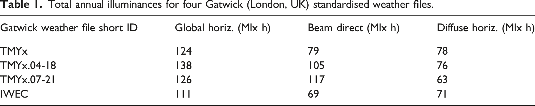
There are marked differences in the annual totals for illuminance. On what basis should the user decide which one of the four to use when evaluating EN 17037 daylighting performance criteria? How to address this question became the impetus for the investigation described in this article. The method devised by the authors was to compare each of the four TMYs against 10 years of recent solar radiation data (2013–2022) derived from satellite remote-sensing observations. And hence to assess if it was possible to identify which of the four TMYs most closely reproduced the distributions in 10 years of observed patterns for: global horizontal, beam normal and diffuse horizontal illuminances. Comparison would be made based on the frequency distributions for a full year of data for each of the three illuminance quantities.

Weather files and other sources of solar radiation data

The two essential weather parameters for CBDM are direct beam irradiance and diffuse horizontal irradiance. A desirable (but not essential) parameter is the dew point temperature. The direct beam and diffuse horizontal irradiances are converted to their illuminance equivalents using a luminous efficacy model. The most commonly used in CBDM is the Perez efficacy model which has distinct formulations for the direct beam and diffuse horizontal components. ⁸ The dew point temperature is desirable because the Perez efficacy model has this in the formulation, though the overall effect on an annual basis is believed to be very small, perhaps insignificant. Until recently, all implementations of the Perez luminous efficacy model in CBDM tools/workflows used a fixed dew point temperature, e.g. 11°C. The sections below give an outline of the basis for the solar radiation data found in standardised weather files (IWEC and TMY), but also that derived from remote sensing, i.e. satellite observations.

IWEC files

International Weather for Energy Calculation (IWEC) files were commissioned by ASHRAE in the early 2000s to provide weather files for worldwide locations other than in the United States and Canada. As the authors of the main report on IWEC state, solar radiation modelling was a fundamental part of the research project as solar radiation was not available as a direct measurement like most other variables, and instead sourced from satellite records. ⁶ The model eventually adopted to derive solar radiation was a combination of the METSTAT model (for all components of clear skies), ⁹ the Kasten model (for global irradiance under cloudy skies) ¹⁰ and the Perez model (for splitting the global component into direct and diffuse parts). ¹¹ Input data included dry-bulb and dew-point temperatures, pressure, Earth-sun geometry, aerosol optical depth and total cloud cover. The model parameters were calibrated against daily radiation data sourced from the World Radiation Data Center (WRDC). Data that form the IWEC database were all collected in the period 1982–1999.

Thevenard and Brunger wisely warned colleagues regarding the dangers of ‘piling up models’: “Even if one hopes that, on average, diffuse illuminance is properly calculated by this succession of models, there is no doubt that a comparison of hourly values contained in the IWEC files to values that would be measured at the same site would not be very good. Unfortunately, there is little that can be done to alleviate this problem; the best that can be done is to use some caution and judgment when using these calculated values.” ⁶

TMYx files

Solar radiation in TMYx files ¹² is sourced from the ERA5 atmospheric reanalysis dataset, produced by the Copernicus Climate Change Service (C3S) at the European Centre for Medium-Range Weather Forecasts (ECMWF). The term ‘reanalysis’ refers to the recombination and crosschecking of historical data coming from the core Numerical Weather Prediction (NWP) model, from ground observations, and from satellite imagery. This postprocessing step improves the accuracy of the initial numerical predictions. The dataset provides hourly values of global horizontal irradiation (called ‘Surface short-wave radiation downwards’) derived from a Radiative Transfer Model, and not directly assimilated by the reanalysis process, i.e. not directly corrected against measurements of solar irradiance at ground level. Global horizontal irradiation, in J/m², can be used to calculate mean global horizontal irradiance centered on the half hour. ¹³ Spatially averaged values are given on a 31 × 31 km grid. ¹⁴

Copernicus CAMS data

The Copernicus Atmosphere Monitoring Service (CAMS) provides freely available satellite-derived radiation data covering Europe, Africa, the Middle East and parts of South America. The period of record is February 2004 to the present day. The CAMS data are provided by the Meteosat Second Generation (MSG) weather satellites which are positioned variously within 10° of the prime meridian (i.e. 0° longitude) in a geostationary orbit ∼36,000 km above the equator. An approximate full-disc view of the Earth from Meteosat 10 is shown in Figure 1. The visible disc has an extent of −66 to 66° in both latitudes and longitudes. Data for locations towards the edge of the field of view are unreliable because cloud properties cannot be determined with sufficient accuracy at large satellite viewing angles. Usable data is generally considered to be that within a region of −60 to 60° in both latitudes and longitudes for satellites positioned at 0° longitude – see bold lines in Figure 1. The following sections give an outline of the CAMS solar radiation data and the justification for using CAMS as a reference source of irradiation data for the derivation of daylight quantities.

Figure 1.

Approximate full disc view of the Earth from Meteosat 10. Dashed lines show parallels of latitude and meridians of longitude both with 30° spacing.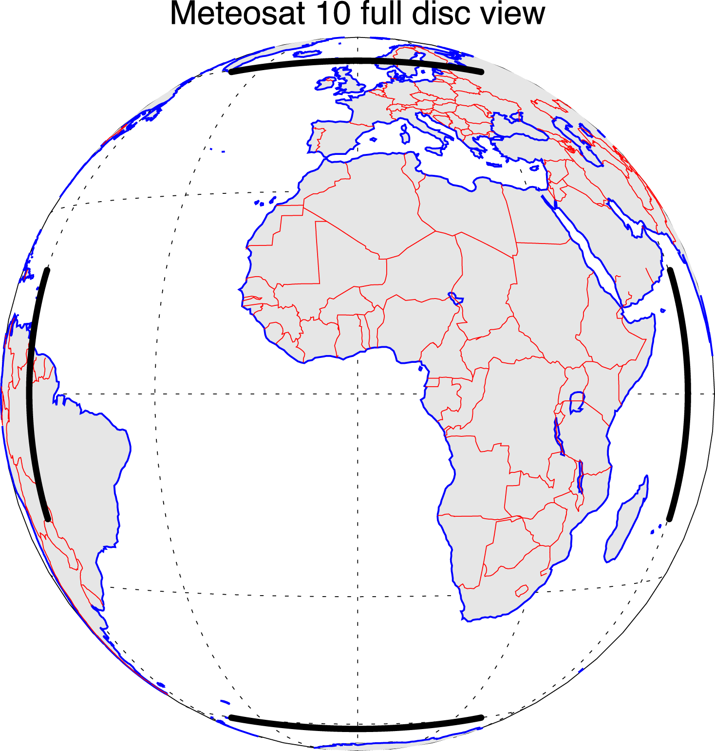

Irradiation data provided by the Copernicus Atmosphere Monitoring Service (CAMS) are based on a combination of the McClear clear sky model and satellite cloud observations (Heliosat-4 method).^15,16 The McClear (v3) physically-based model takes data provided by the CAMS global forecast and reanalysis on aerosols, ozone and water vapour column content, and the surface reflective properties as inputs; these are used to derive global and direct irradiation under cloud-free conditions. ¹⁷

To provide irradiation data for all sky types, the clear-sky results are then combined with cloud information extracted by satellite imagery and processed by the McCloud model. The validation of the Heliosat-4 method against irradiance values measured at 13 stations from the Baseline Surface Radiation Network (BSRN) found overestimating biases between 0–12% and RMSEs between 15–43% for the global component, and biases between −40 and +8%, with RMSEs between 26–85% for the direct component. These ranges include locations at the edge of the satellite viewing angles (Northern Europe, above latitudes of 58°), which are affected by larger parallax errors and by the presence of persistent snow. For all other locations, direct irradiance is estimated with biases between -19–8% and RMSEs between 26–53%. ¹⁵

While ground measurements and reanalysis datasets provide cumulative irradiation values over each of the considered time steps, satellite data are formed by instantaneous ‘snapshots’ taken at the time of the image capture. Values for a specific location are bi-linearly interpolated from a 4 × 4 km grid. ¹⁴ Salazar et al. ¹⁴ performed a thorough comparison study of satellite and reanalysis models, assessed against irradiance values measured at the BSRN station of Petrolina (BR). Results indicated a better overall performance of CAMS data than ERA5 data, in particular for estimates of direct sunlight irradiance. This finding was confirmed at other locations, e.g. by a study conducted with data from Spain and Switzerland. ¹⁸

Rationale for using CAMS as a reference source of daylight data

Given the aforementioned good agreement between CAMS irradiation data and ground measurements, the use of illuminance data derived from CAMS would appear to be a potentially valuable resource for the characterisation and simulation of actually occurring daylight conditions. To test this hypothesis, illumination values derived from 60 and 15 min CAMS irradiation data were compared against ground measurements for 610 full days taken sequentially at three locations in the UK during the years 2015, 2016, 2019 and 2022. The validation methodology and a summary of the results are described below. The complete set of 610 daily plots is included as Supplemental Data to this article (available online).

Method I: the validation dataset

Beginning in 2015, Mardaljevic and Cannon-Brookes carried out a series of daylight conservation projects in partnership with the National Trust (UK).^19–21 In addition to monitoring internal illumination conditions, external daylight conditions were measured using a BF5 Sunshine Sensor produced by Delta-T Devices (Cambridge, UK). The BF5 Sunshine Sensor is a solid-state device with no moving parts, Figure 2.

Figure 2.

BF5 device in the grounds of Ickworth House (2015).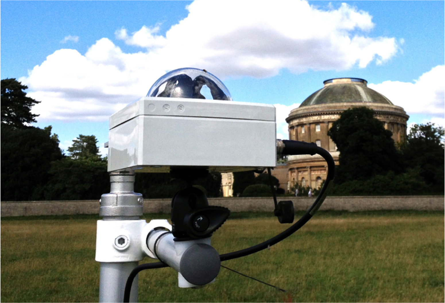

The BF5 has an array of photodiodes together with a shading pattern to measure incident solar radiation from which the device calculates global horizontal and diffuse horizontal illuminance. A validation of an earlier Delta-T instrument (BF3) using similar technology but measuring irradiance was published in 2003. ²² For illuminance, the BF5 device has a claimed relative accuracy of ±12% for global horizontal and ±15% for diffuse horizontal, and an absolute accuracy of ±0.600 klx for both quantities. The resolution is given as 0.060 klx, i.e. 60 lx.

The locations

The National Trust used the BF5 device to record external conditions at 1 min intervals for three locations in England: Ickworth House (Bury St Edmunds), Ham House (London) and Belton House (Grantham), Table 2. In total, there were 610 complete days of 1 min measurements: 191 days and 180 days at Ickworth House (in 2015 and 2016, respectively); 123 days at Ham House (in 2019); and, 116 days at Belton House (in 2022). For each location, the BF5 was sited in a position that had a largely unshaded view of the entire sky dome.

Table 2.

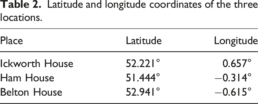
Latitude and longitude coordinates of the three locations.

Place	Latitude	Longitude
Ickworth House	52.221°	0.657°
Ham House	51.444°	−0.314°
Belton House	52.941°	−0.615°

Converting CAMS irradiance values to illuminance

Annual 60 min and 15 min CAMS data were downloaded from the Soda-Pro.com portal for the three locations: Ickworth (2015 and 2016); Ham House (2019; and, Belton House (2022). Global horizontal illuminance $E_g^{\mathit{CAM}}$ was derived from CAMS values for diffuse horizontal irradiance $I_d^{\mathit{CAM}}$ and beam normal irradiance $I_b^{\mathit{CAM}}$ as follows:

$E_g^{\mathit{CAM}}=K_d{I}_d^{\mathit{CAM}}+\left(K_b{I}_b^{\mathit{CAM}}\right)\sin \alpha$

(1)

where K _d and K _b are, respectively, the (instantaneous) luminous efficacy coefficients for diffuse and beam radiation calculated using the Perez models, and α is the solar elevation. ⁸ The diffuse horizontal illuminance $E_d^{\mathit{CAM}}$ shown in the daily plots is, of course, equal to the first term following the equals sign. A fixed dew point temperature of 11°C was used for the conversion of CAMS irradiation because temperature data are not available directly from the Soda-Pro.com portal. However, the dew point temperature is known to be a small factor in the conversion of irradiance to illuminance, ²³ and its significance unlikely to be detectable given the error characteristics of the BF5.

Compiling the validation dataset

Only complete days of data for both CAMS and BF5 were included in the validation dataset. As expected, the dowloaded CAMS data did not contain any missing irradiance values at either the 60 min or 15 min time-steps. For the 1 min BF5 data, only days with 24 × 60=1440 values recorded were included in the dataset. For three of the four years, the BF5 time stamp needed to be corrected by 1 hr to convert from BST to GMT. The BF5 1 min data were averaged across 15 min and 60 min periods for comparison with the respective CAMS data. For the 15 min daily plots, the mid-point of the time increment was used, e.g. the 7¹/₂, 22¹/₂, 37¹/₂ and 52¹/₂ minute marks. There was no noticeable drift in the BF5 clock, e.g. from conspicuous misalignment with CAMS on clear sky days.

Results I: validation of CAMS-derived illuminance data

The validation focuses on the comparison of GHI measured directly by the BF5 with GHI derived from CAMS diffuse horizontal and beam normal irradiance data. The presentation of results comprises six parts:

1. A brief discussion of ten sample daily plots of GHI selected to illustrate the various types of sky conditions found in the dataset.

2. Evaluation of GHI daily totals for all 610 days – scatter plot and table.

3. Evaluation of 60 min GHI data – density map scatter plot and table.

4. Evaluation of 15 min GHI data – density map scatter plot and table.

5. Evaluation of the daily variability in GHI for both 60 min and 15 min GHI data – scatter plot and tables.

6. The full set of 610 daily plots – Supplemental Data available online.

Ten example GHI daily plots

Example comparisons between the BF5 measurements for GHI with CAMS-derived illuminance data for ten days are shown Figure 3. The 1 min BF5 data were averaged to 15 min intervals and plotted together with 15 min CAMS-derived illuminances. The ten days were selected to show the range in the agreement obtained – the sample should not be taken to be representative of the 610 days. The plots also show DHI, largely to indicate when the contribution of BNI was present. The day number shown on the daily plots (top right) is the Julian day number JD reset to 1st January 2015:

$\text{Day\hspace{0.17em}number}=JD-J{D}^{1/1/2015}+1$

(2)

Figure 3.

Sample ten days comparison of BF5 measurements (red curves) with CAMS-derived illuminance data (blue curves) for GHI (solid lines) and DHI (dashed lines).

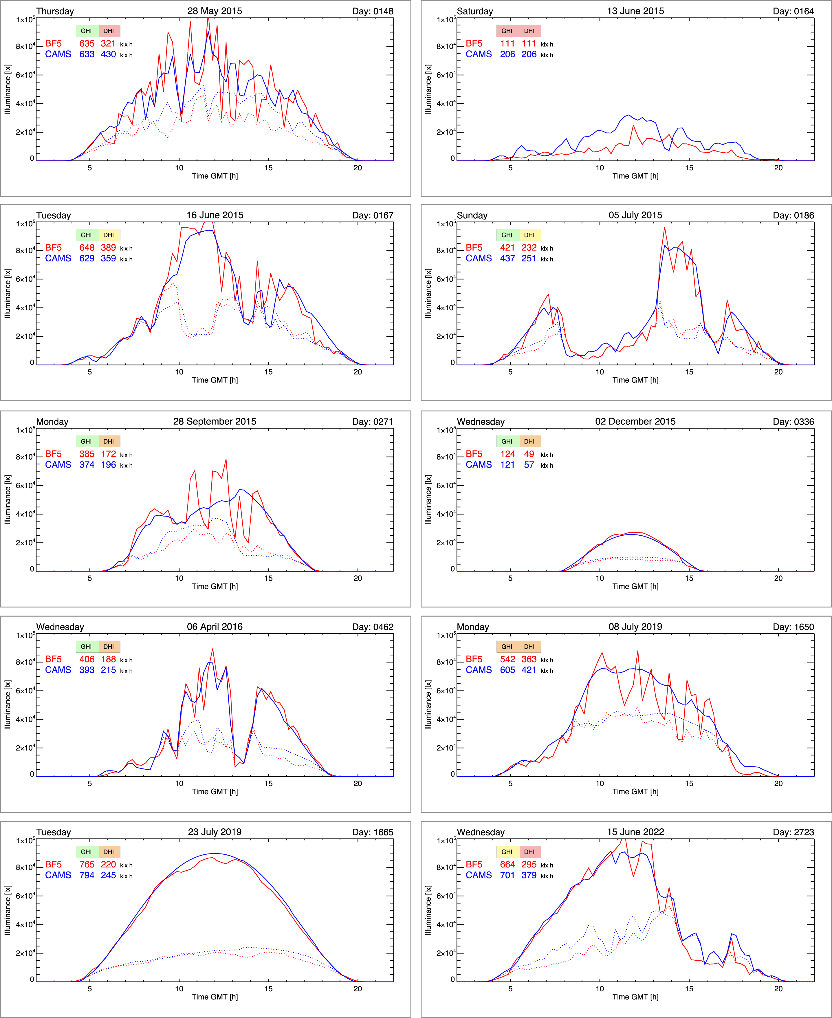
Each plot is annotated with the daily totals for GHI and DHI (units klx h). To aid speedy assimilation of the agreement in the daily totals, the GHI and DHI text annotations are shaded to show the percentage difference in four ranges:

• Green shading for agreement better than 5%.

• Yellow shading for agreement in the range 5% to 10%.

• Amber shading for agreement in the range 10% to 25%.

• Red shading for agreement worse than 25%.

Thus, the green and yellow shades indicate where, for all practical purposes, the BF5 and CAMS daily totals are considered to be in full agreement within the limits of what can decided on the basis of ‘ground truth’ validation results, i.e. within ±10%.

Day 0148 shows a fairly bright spring day with marked short timescale ( $<$ 1 hr) variability in GHI. For some of the variation the CAMS (GHI) time-series is closely aligned with the BF5, e.g. between 09:00 and 12:00, though the amplitude of BF5 variability is generally greater than that for CAMS. The GHI daily totals agree within ±5%.

Day 0164 was a particularly dull/overcast day for June, with no detectable BNI component. The CAMS GHI values are markedly greater than that measured on the ground.

Days 0167, 0186 and 0462 all show distinct periods of fully overcast and largely clear skies. Variability is pronounced, with transitions between overcast and clear skies occurring at the time-step scale, i.e. 15 mins. Notwithstanding this variability, the CAMS GHI curves closely follow those of the ground measurements. The GHI daily totals for these three days all agree within ±5%.

Days 0271 and 1650 exhibit short-term variability, but without distinct overcast and largely clear sky periods. For these two days, the CAMS curves follow the prevailing pattern of the BF5 curves, but without closely following the short-term variability. Nevertheless, the differences in GHI totals are still small: within ±5% (day 0271) and just outside the ±10% range, i.e. 11.8% (day 1650).

Days 0336 (winter) and 1665 (summer) both exhibit typical ‘bell-curve’ clear-sky GHI diurnal patterns, with only tiny ‘wiggles’ in the BF5 measurements showing minimal deviation from the ideal curve shape. The GHI daily totals for both days agree within ±5%.

Lastly, day 2723 (six days short of the summer solstice) shows largely clear sky conditions from shortly after dawn until around 11:00 when partial clouds become evident. From around 14:00 the sky becomes largely overcast. The GHI daily totals agree within ±10%.

For the daily 15 min time-series plots discussed above (plus the other 600 in the Supplemental Data), the authors were more than a little surprised at the remarkably good agreement between the CAMS-derived GHI and the BF5 measurements. In particular, the often close alignment between the curves on a sub-hourly scale for days with partial/transient cloud was not expected given the potential for geostationary remote sensing observations to be affected by parallax.

Daily total GHI

A scatter plot of daily total GHI for 15 min averaged BF5 data and 15 min CAMS GHI (derived from BNI and DHI irradiation values) data for all 610 days is given in Figure 4. The dashed green lines show the ±10% and ±25% boundaries relative to the equality line.

Figure 4.

Scatter plot of daily total GHI for BF5 measurements against CAMS 15 min GHI derived from beam normal and diffuse horizontal irradiances.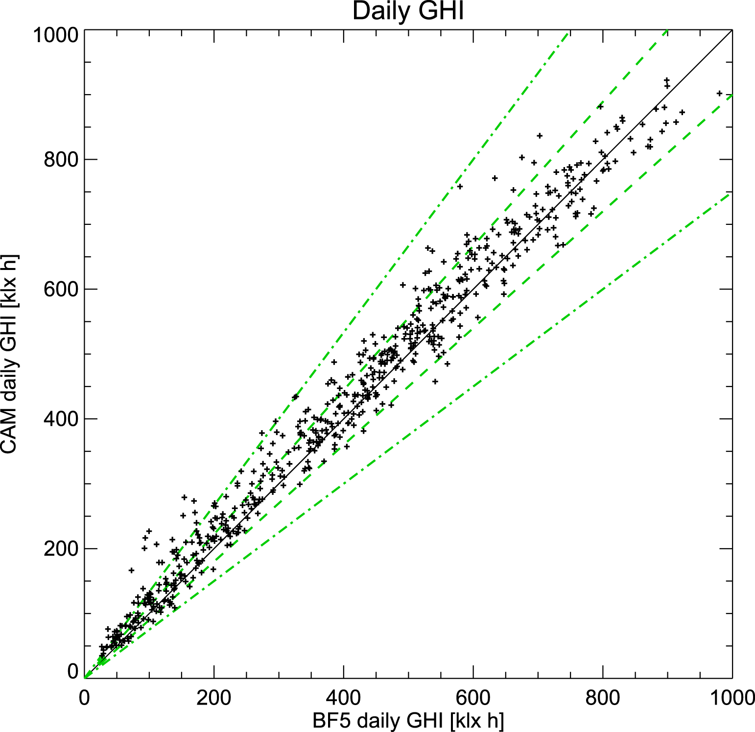

The overall mean bias and root mean square percentage errors in CAMS daily totals relative to BF5 measurements are given in Table 3. The first row is for the entire validation dataset of 610 days – the MBE is 9.0% and the RMSE 10.0%. Which can be considered to be good agreement. The subsequent rows sub-sample the dataset to include only those data pairs where the BF5 daily total exceeded the value shown in the first column. For example, when the BF5 daily total GHI condition is 100 klx h (second row), the number of data pairs reduces from to 545 (from 610). For GHI daily totals of increasing magnitude, the contribution of BNI to the CAMS-derived GHI totals will, of course, become increasingly more important. The trend which is visible in the scatter plot (Figure 4) becomes much clearer in Table 3: the MBE gradually diminishes from 9.0% to less than ±2%, and the RMSE from 10.0% to 4.1%.

Table 3.

Daily total GHI errors for 15 min data.

GHI Day > (klx h)	N data pairs	MBE (%)	RMSE (%)
0	610	9.0	10.0
100	545	6.4	9.3
200	456	4.7	8.4
300	388	3.8	7.8
400	315	3.2	7.3
500	222	2.7	7.0
600	126	1.2	5.7
700	72	−0.4	4.8
800	25	−1.6	4.1

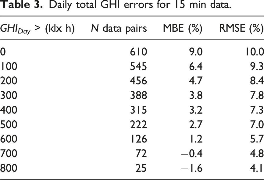
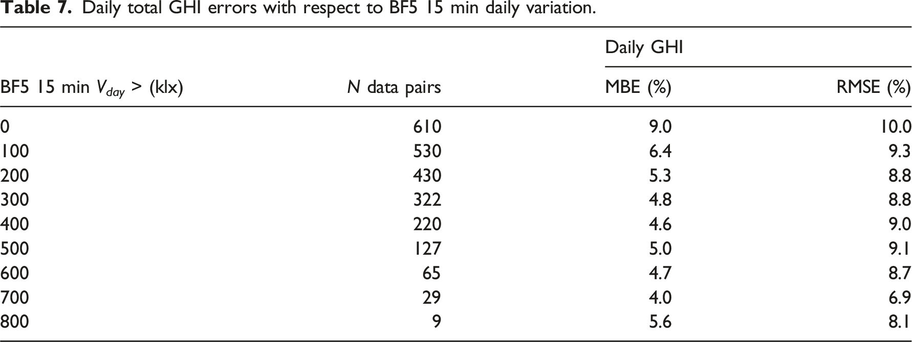
The purpose here is to demonstrate that the agreement, which is already good when the entire dataset is considered, becomes no worse when only those days with high levels of sunlight are selected. In fact, the opposite is clearly the case: the agreement improves to a degree which must be considered quite remarkable for a direct comparison of satellite-derived illuminance values against ground measured data.

Comparison of 60 min and 15 min GHI

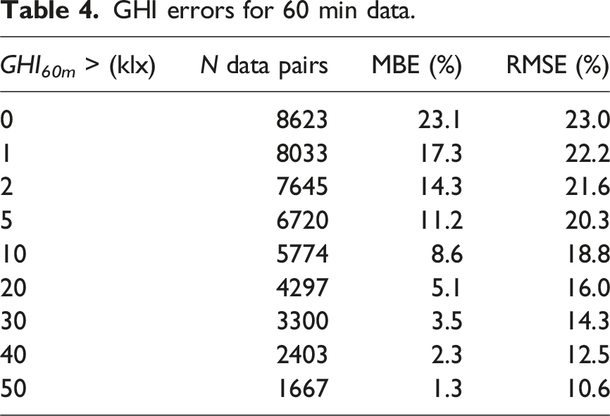
In this section the time-step GHI values for all 610 days are compared for two cases:

i. 60 min (i.e. hourly) CAMS-derived illuminance data against 60 min averaged BF5 measurements; and,

ii. 15 min CAMS-derived illuminance data against 15 min averaged BF5 measurements.

The scatter plot data are presented as density maps given the high number of data pairs: 8623 for the 60 min time-step, and 33,235 data pairs for 15 min time-step. The density map for the 60 min time-step data is shown in Figure 5. The bin size is 2.5 klx, and the colour scale mapping for the density plot is logarithmic with a range from 10 to 250 data points. Bins containing a number of data points between 1 and 4 are shaded light grey, and those in the range 5–9 are shaded dark grey. The dashed green lines show the ±10% and ±25% boundaries relative to the equality line. Judging from visual impression, the agreement appears largely good, with the scatter tending to decrease for higher values of GHI, i.e. for values 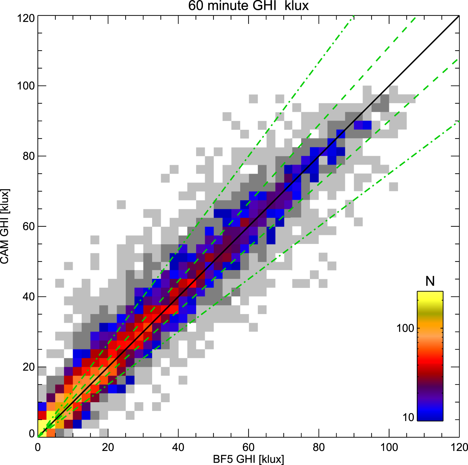$>$ 40 klx.

Figure 5.

Density map for GHI scatter plot of CAMS versus BF5 for 60 min data (8623 points).

Similar to what was done for the daily GHI totals, the overall MBE and RMSE numerical values are shown in Table 4 for all data pairs (row 1), and for subsequent rows where the BF5 GHI value exceeds the amount shown in the first column. For all 8623 data pairs, the MBE was 23.1% and the RMSE 23.0%. Given that the absolute precision of the BF5 device was stated as ±0.600 klx, GHI values below 1 or 2 klx must be considered unreliable. Indeed, removing those data pairs where the (BF5) GHI is less than 2 klx reduces the MBE to 14.3% (with also a marginal improvement in RMSE – row 3 Table 4). Considering the 5774 data pairs for (BF5) GHI greater than 10 klx, the MBE reduces to 8.6% and the RMSE to 18.8%. With each additional 10 klx increment the MBE and RMSE values steadily diminish, reaching a remarkably low MBE of 1.3% and RMSE of 10.6% for the 1667 data pairs where the (BF5) GHI are greater than 50 klx.

Table 4.

GHI errors for 60 min data.

GHI 60m > (klx)	N data pairs	MBE (%)	RMSE (%)
0	8623	23.1	23.0
1	8033	17.3	22.2
2	7645	14.3	21.6
5	6720	11.2	20.3
10	5774	8.6	18.8
20	4297	5.1	16.0
30	3300	3.5	14.3
40	2403	2.3	12.5
50	1667	1.3	10.6

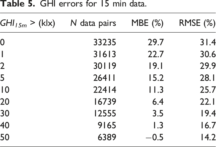
Repeating the evaluation for the 15 min time-step data, results in a similar density plot, but with visibly greater scatter, Figure 6. The total number of data pairs is 33,235, and so the logarithmic colour scale now covers the range 10 to 1000. The bins containing 1 to 9 points are shaded grey as before.

Figure 6.

Density map for GHI scatter plot of CAMS versus BF5 for 15 min data (33,235 points).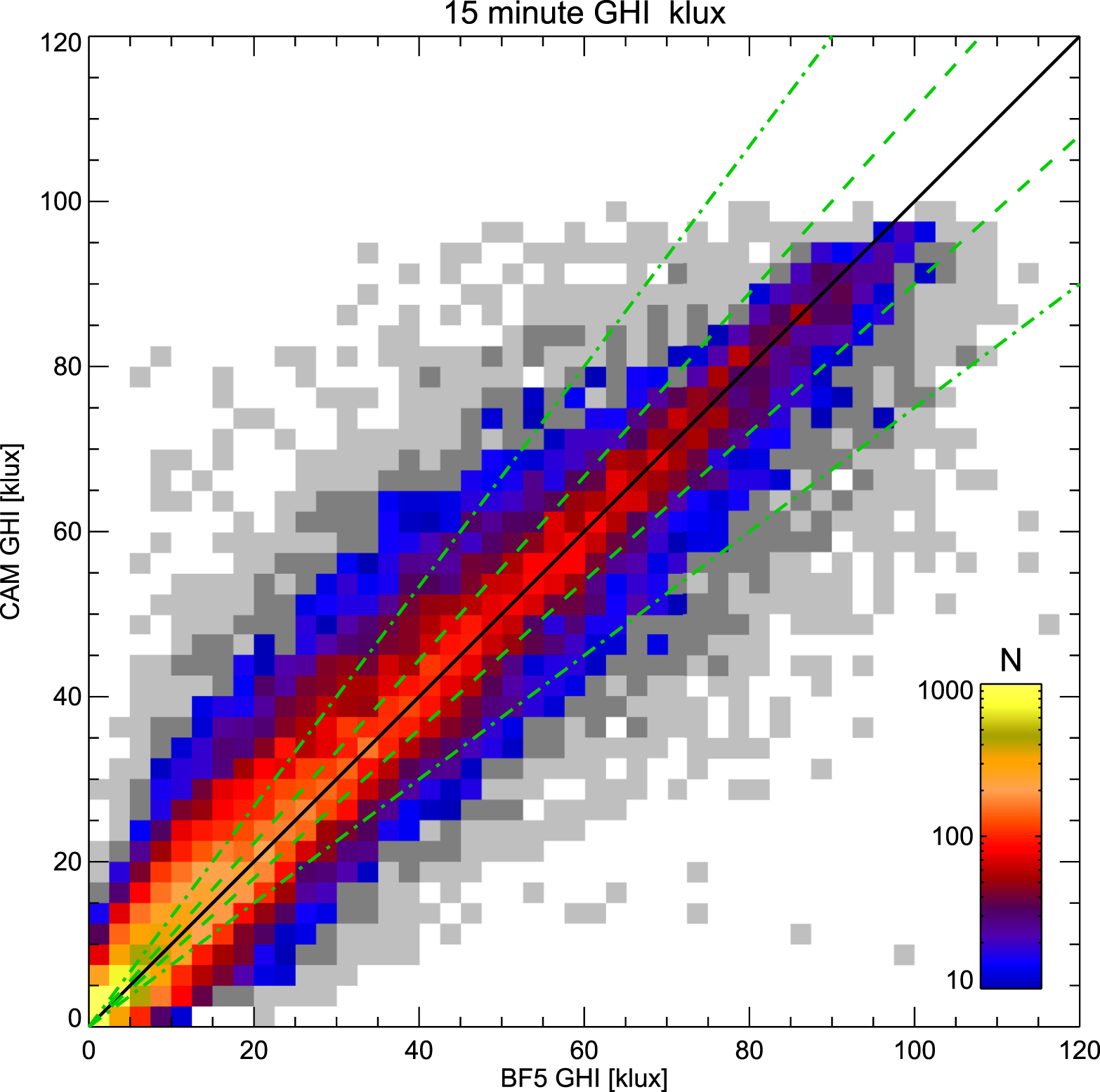

The MBE and RMSE data in Table 5 follows the same form as the previous table for the 60 min data. The row 1 values for all 33,235 data pairs gives an MBE of 29.7% and an RMSE of 31.4% – markedly higher than the comparative values of the 60 min data. However, considering only those data pairs where (BF5) GHI is greater than 10 klx, the difference narrows: MBE/RMSE now 11.3%/25.7% (15 min data) against 8.6%/18.8% (60 min data). For progressively higher GHI values, the MBE values for 15 min data actually converge to those of 60 min data, i.e. they become negligible. And, for GHI greater than 50 klx, the RMSE value for 15 min data (14.2%) is only marginally higher than that for 60 min data (10.6%) even though there are ∼4 times as many data pairs in the 15 min data. An outcome that the authors did not expect.

Table 5.

GHI errors for 15 min data.

GHI 15m > (klx)	N data pairs	MBE (%)	RMSE (%)
0	33235	29.7	31.4
1	31613	22.7	30.6
2	30119	19.1	29.9
5	26411	15.2	28.1
10	22414	11.3	25.7
20	16739	6.4	22.1
30	12555	3.5	19.4
40	9165	1.3	16.7
50	6389	−0.5	14.2

Daily variability in GHI: 60 and 15 min

The final part of the validation section is an examination of differences in daily variation of GHI between the 60 min and 15 min time-steps for the CAMS and BF5 datasets. The measure of daily variation (V _day ) is illustrated in Figure 7 which shows a hypothetical GHI time-series for days n and m. The changes in GHI are marked by the δ labels. The total variation V in GHI for either day is simply the sum of the absolute value for all the time-step changes in the GHI time-series for that day:

$V_{\mathit{day}}=\sum _{\mathit{day}}|\delta E_i|$

(3)

Figure 7.

Illustration of daily variability in GHI as the sum of incremental changes during the day.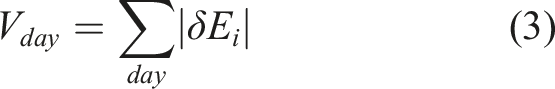

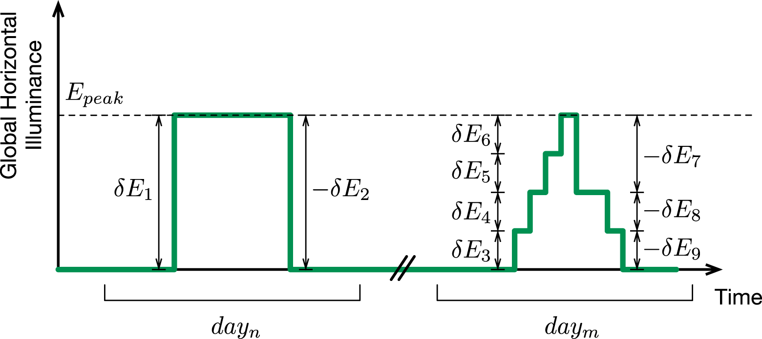
Evidently, for day n the total variation is:

$V_n=\delta E_1+|-\delta E_2|=2E_1$

(4)

Also evident is the observation that the variation for both days shown in Figure 7 must be the same, i.e. V _n = V _m . Thus, provided the change in GHI (for any particular day) exhibits a monotonic rise, reaching a maximum E _peak , and then followed by a monotonic decrease, the numerical measure of time-step variation for that day V _day will always equal twice E _peak irrespective of the time-step or any of the rates-of-change. This idealised condition does in fact occur in the dataset, and almost exactly for all practical purposes – but only for very clear days where the sun is unobscured by any cloud from dawn to dusk. i.e. the ‘classic’ clear-sky bell-shaped curve for GHI (see days 0336 and 1665 in Figure 3 for a close approximation).

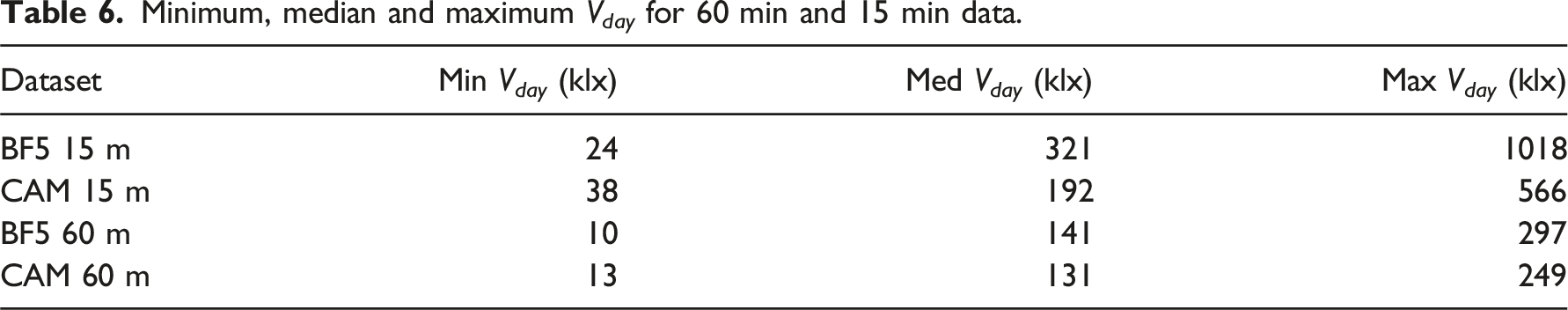
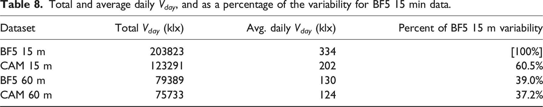
The V _day metric was used to compare measures of daily variation in GHI for the BF5 and CAMS datasets using both 60 min and 15 min data. The scatter plots for both 60 min and 15 min data are shown in the same plot, Figure 8. The 60 min data pairs are plotted using a small red square, and the 15 min data using a small black cross symbol. Firstly, the 60 min data points are largely clustered around the equality line, with a maximum daily variation less than 300 klx. The 15 min data cover a much larger range with a larger scatter. The higher values greater than 300 klx are typically below the equality, i.e. the CAMS measures of V _day are generally smaller than that measured by the BF5. The minimum, median and maximum V _day values for the four datasets are summarised in Table 6.

Figure 8.

Scatter plot of GHI daily variation for CAMS versus BF5 for 60 min and 15 min data, plus 15 min GHI time-series plots for three illustrative days.

Table 6.

Minimum, median and maximum V _day for 60 min and 15 min data.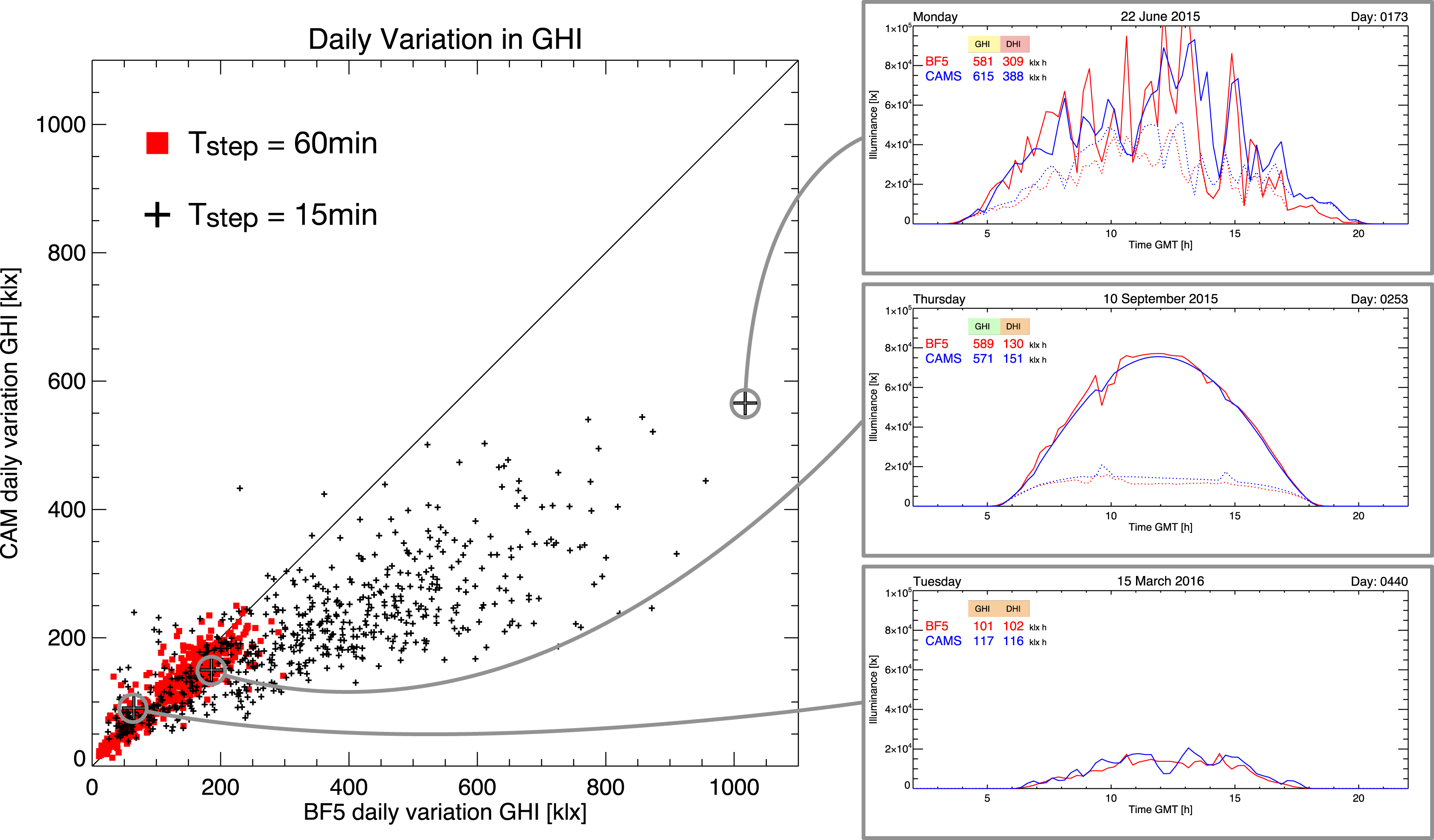

Dataset	Min V day (klx)	Med V day (klx)	Max V day (klx)
BF5 15 m	24	321	1018
CAM 15 m	38	192	566
BF5 60 m	10	141	297
CAM 60 m	13	131	249

To the right of the scatter plot are 3 days illustrating different types of variability. Each daily plot has a grey line which ‘connects’ the daily time-series to the corresponding datapoint on the scatter plot. The topmost plot is for day 0173 (22nd June 2015). This day had the highest recorded V _day value. It can be seen in the daily plot that the amplitude of variability in the CAMS data is less than that for the BF5 – hence that data point falls markedly short of the equality line in the scatter plot. However, the daily total GHI for CAMS (615 klx h) is still within ±10% of the BF5 value (581 klx h). The middle plot is for day 0235 (10th September 2015) – a clear sky day with an almost ideal GHI ‘bell curve’ for the CAMS data, and a small degree of variability shown in the BF5 time-series. Here, the GHI daily totals are within ±5% (i.e. green shade for GHI label). As noted above, for such curves the daily variability is approximately twice the peak GHI value. The bottom-most curve is for a very dull day: 0440 (15th March 2016). The GHI daily total is only 101 klx h (BF5), and the CAMS value is 117 klx h – the agreement falling just outside the ±10% range (amber shading).

Thus far, for both the 60 and 15 min data, the time-step agreement between CAMS and BF5 data-pairs improved markedly as the GHI values increased – see Tables 4 and 5. For days with high degrees of variability (such as day 0173 – Figure 8), one would not expect the 15 min time-step data points to show good agreement. However, does higher daily variability in GHI lead to increasing MBE/RMSE in the daily totals of GHI? In other words, does higher daily variability tend to lead to a systematic bias and/or greater scatter in the daily totals for GHI? This hypothesis was tested by calculating the daily GHI MBE/RMSE values for those days where the (BF5 15 min) V _day exceeded a threshold value: from 0 klx (i.e. all the data points) to 800 klx in steps of 100 klx. The results are shown in Table 7. Since the minimum V _day was, of course, greater than zero, the first row of Table 7 is identical to the first row of Table 3. The 80 days where 0 < V _day < 100 will tend to be those with lowest levels of GHI. Excluding those, the daily MBE in GHI improves from 9.0% to 6.4%. For those days where V _day > 200 klx, the MBE (in daily GHI) reduces further to 5.3%. Thereafter, the MBE fluctuates slightly, but staying within the range 4.0% to 5.6%. Contrary to what one might expect when comparing 15 min satellite-derived illuminance data with ground measurements, those days which exhibit the highest degree of (15 min) variability nevertheless still result in GHI daily totals that show a remarkable degree of agreement, i.e. MBE values around 5%. In other words, whilst the CAMS data cannot reproduce the full extent of GHI variability as measured on the ground, the agreement in daily total GHI values is still very good. Thus, what was shown in the illustration (day 0173 in Figure 8) is, in fact, typical of the entire sample: the CAMS peaks and troughs might not match the full extent of those recorded by the BF5, but that does not introduce an overall bias in the daily levels. This is an important finding for what follows in part II of the article.

Table 7.

Daily total GHI errors with respect to BF5 15 min daily variation.

BF5 15 min V day > (klx)	N data pairs	Daily GHI
		MBE (%)	RMSE (%)
0	610	9.0	10.0
100	530	6.4	9.3
200	430	5.3	8.8
300	322	4.8	8.8
400	220	4.6	9.0
500	127	5.0	9.1
600	65	4.7	8.7
700	29	4.0	6.9
800	9	5.6	8.1

This section concludes with a comparison of total V _day (i.e. all 610 days) for all four datasets. The results are shown in Table 8. The average daily V _day is simply the dataset total divided by 610. The final column expresses the variability as a percentage of that exhibited by the BF5 15 min data. For the 60 min data, the difference between BF5 and CAMS variability is negligible. For the 15 min data, the BF5 variability is markedly greater than the CAMS variability. Nevertheless, the 15 min CAMS variability is also markedly greater than either of the 60 min datasets. In relative terms, the (15 min) CAMS variability is $\sim 1.5\times$ that of the 60 min data (i.e.  $\sim 50$ % greater). The significance of this for compiling AMY solar data will be discussed following the part II Method and Results below.

Table 8.

Total and average daily V _day , and as a percentage of the variability for BF5 15 min data.

Dataset	Total V day (klx)	Avg. daily V day (klx)	Percent of BF5 15 m variability
BF5 15 m	203823	334	[100%]
CAM 15 m	123291	202	60.5%
BF5 60 m	79389	130	39.0%
CAM 60 m	75733	124	37.2%

Summary of validation results

In short, the authors were more than a little surprised at the remarkably good agreement between the CAMS data and the BF5 measurements for GHI. In particular, the often close alignment between the curves on a sub-hourly scale for days with partial/transient cloud was not expected given the potential for remote sensing observations to be affected by parallax. At latitudes between 51.444° and 52.941° (less than 10° away from the 60° cutoff), the data for these three places are likely to be affected more by parallax than lower latitude locations.

As noted, the CAMS GHI illuminance values were derived from the CAMS beam normal and CAMS diffuse horizontal irradiance data. Consequently, we consider the very good agreement with the BF5 GHI ground measurements to offer convincing, albeit indirect, validation of both the beam normal and the diffuse horizontal irradiance data supplied by CAMS.

For the comparison of annual weather datasets that follows in Part II of the article, we believe that the validation described above amply justifies the assertion that CAMS-derived illuminance data are indeed a reliable indicator of long-term actually occurring sunlight (i.e. BNI) and skylight (i.e. DHI) daylight conditions.

Note, the first of Meteosat’s Third Generation Imager (MTG-I) series of satellites became fully operational in December 2024. Now designated Meteosat-12, full disc images of the Earth are captured every 10 min, rather than every 15 min for the previous generation of Meteosat imaging satellites. A second MTG-I satellite is scheduled for launch in 2026 which will acquire images of just Europe every 2.5 min. Spatial resolution will also be improved. Although not yet confirmed, it seems likely that ground irradiation data derived from the more frequent sampling of the Third Generation Imager satellites will eventually become available.

CAMS as a daylight resource

The application of CAMS data for the evaluation of TMY solar data and daylight modelling purposes is described in the Discussion section toward the end of the article. However, it should be noted that the validation described here shows CAMS to be a high-quality daylight resource, the value of which appears to have been overlooked until now. There is now considerable research activity to quantify the so-called non-image forming (NIF) effects of illumination on humans, for example, circadian photoentrainment. ²⁴ Personal light exposure field studies involving subjects wearing illumination recording devices to determine the light received by the eye are now commonplace. ²⁵ However, unless there was a dedicated (or available) weather station nearby that recorded, say, GHI, daylight conditions during the field study could not be reported. This confounds attempts to apportion the relative and/or absolute contributions of daylight and electric light to personal light exposure. For personal light exposure studies carried out within the CAMS region of coverage, the CAMS irradiation data could be used to derive ‘boundary’ (i.e. outside) daylight conditions. In order to make use of CAMS as a post hoc source of daylight data, the addition of lat/lon location information to the standard protocol for reporting personal light exposure studies has been proposed. ²⁶

Method II: comparison of weather files

The weather file locations selected for the analysis described here were Gatwick (London, UK), Fiumicino (Rome, IT) and Arlanda (Stockholm, SW). For each of these locations there were four standardised weather files available: three from Climate OneBuilding and one from the Energy Plus websites. For each location a full decade of AMYs (2013-2022) were compiled using both 60 min and 15 min CAMS data. Thus there were 24 weather files for each location; 72 weather files in total. Hereafter, the term AMY(s) is used to refer the 60 files generated from CAMS data as a basis for CBDM simulations. The labelling for the CAMS data gives the time-step and the year, e.g. C15M-2013 refers to a 15 min time-step AMY for the year 2013. The term IWEC is used to refer to the three weather files from the Energy Plus website. The term TMYx is used to refer to any of the nine weather files from the Climate OneBuilding Web site. Lastly, as noted earlier, the term TMY(s) is user to refer to the TMYx and/or the IWEC standardised weather files.

Compiling AMYs from CAMS data

CAMS radiation data were sourced from the Soda-Pro.com portal. The site-specific inputs required are: latitude; longitude; altitude; start date; end date; time-step (1 min, 15 min, 60 min, day or month); and, time reference (universal time or true solar time). The data can be downloaded manually using the website interface, or via custom written scripts. The latter approach was chosen for efficiency – 60 CAMS-derived AMYs were created for this investigation.

At first it was decided to create AMYs based on 60 min time-step CAMS data, i.e. commensurate with the hourly time-step of standardised weather files. However, the aforementioned validation revealed remarkably good time alignment between 15 min CAMS data and ground measurements (see Figure 3). Accordingly, it was decided to create 10 years of AMYs using CAMS data at both the 60 min and 15 min time-steps, i.e. 20 AMY files per location. Whilst it was to be expected that 60 min and 15 min CAMS AMYs should have largely identical characteristics, as far as we are aware this had not been tested for the comparative method (i.e. frequency histograms) described in the next section.

The parameters extracted from the CAMS data for the CBDM AMYs were: year; month; day; hour; minute; global horizontal irradiation (Wh/m²); beam irradiation on horizontal plane (Wh/m²); diffuse horizontal irradiation (Wh/m²); beam normal irradiation (Wh/m²); and, a reliability flag. The sun altitude and azimuth were calculated from the time-stamp and location information, and routine consistency checks performed on the data. No issues were encountered. For leap years, data for 29th February were removed to ensure all AMYs contained data for 365 days – the same as the TMY weather files.

Converting irradiance to illuminance: AMYs and TMYs

For both the AMYs and TMYs, diffuse horizontal and beam normal illuminance values were derived from irradiance (or irradiation) using, respectively, the Perez luminous efficacy models for diffuse and beam radiation. ⁸ Since the TMY files contained the time-series for dew point temperature, this factor was included in the efficacy models. Whereas a fixed dew point temperature of 11°C was used for the CAMS AMYs. As noted, the effect of including this factor is known not to be significant. ²³

Global horizontal illuminance was determined as the sum of diffuse horizontal illuminance and the horizontal component of beam normal illuminance. This is preferred to using the simpler one-step approach of applying the Perez luminous efficacy model for global radiation because the global model is inherently less reliable than applying the individual component models. Hereafter, the terms GHI, BNI and DHI are used, respectively, to refer to global horizontal illuminance, beam normal illuminance and diffuse horizontal illuminance.

Annual illuminance frequency distributions

Frequency histograms for GHI, BNI and DHI were determined for all 72 weather files. The first part of the analysis was largely visual. For each location, the frequency data for GHI, BNI and DHI in turn, were superposed to allow for visual comparison of the various weather files. The histogram data were plotted as frequency polygons since this gives a clearer representation of similarities/differences in the distributions. A bin width of 5000 lx was used, and the bin centre was used as the abscissa point for plotting the frequency polygons. Thus, the first abscissa point for the polygon is plotted at the 2500 lx mark.

Pairwise comparison of frequency distributions

The numerical measure of similarity (or difference) between any two illuminance frequency histograms for a particular location is based on the sum of the absolute differences between the two histograms. In the absence of a justification for determining a population mean for the weather files that can be guaranteed to be without bias, it was decided that all numerical evaluations would be on a pairwise basis. Consider the illustration of a generalised example shown in Figure 9. The abscissa scale x denotes an illuminance quantity, say global horizontal illuminance (GHI) which will typically have a maximum around 100,000 lx for UK weather files. The red and green lines delineate the frequency histograms for the (binned) degree of occurrence (e.g. number of hours) of GHI for weather files r and g, respectively. The bin size is Δx and, for a distribution with n bins, the magnitude of x at the bin centres is indicated using the bin number, i.e. x₁, x₂ up to x _n . Thus, at bin b, the bin centre has an illuminance value x _b and the number of hours where an illuminance value from each distribution ‘falls into’ bin b are r _b and g _b for weather files r and g, respectively. There is considerable variance between the weather files for the frequency occurrence in the first non-zero bin of the distributions. Hence the first bin is excluded from the summations of the absolute difference between any two weather files.

Figure 9.

Illustration showing calculation of the ‘distance’ between the distributions for weather files labelled r (red) and g (green).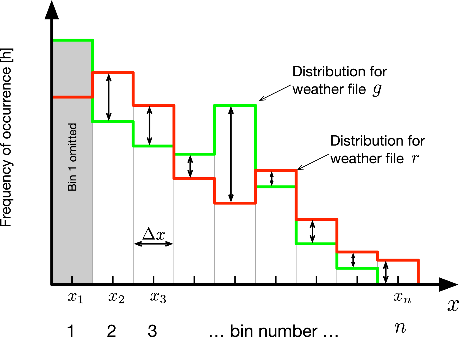

The numerical measures of difference between any two distributions r and g are quantified in two ways:

1. The sum in hours of the absolute difference $D_{rg}^N$ in the frequency of occurrence of an illuminance quantity in each bin for weather files r and g.

2. The sum in lux hours of the absolute difference $D_{rg}^M$ in the magnitude of the illuminance quantity in each bin for weather files r and g.

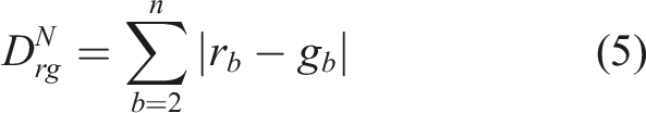
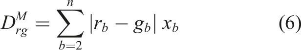
The formulation used to calculate $D_{rg}^N$ is therefore:

$D_{rg}^N=\sum _{b=2}^n|r_b-g_b|$

(5)

whereas, for the magnitude quantity $D_{rg}^M$ , the difference per bin can be estimated as the absolute difference in number of hours (per bin) times the illuminance at the bin centre, Thus, the magnitude sum can be calculated using:

$D_{rg}^M=\sum _{b=2}^n|r_b-g_b|x_b$

(6)

This is an estimate since, all the individual occurrences within any particular bin b will have a range of illuminance values Δx centred on x _b . For the work described in this paper, an exact calculation was used rather than equation (6). However the discrepancy between the exact calculation and the estimate turned out to be negligible, and so the more compact formulation (equation (6)) is given for brevity. Hereafter, the various plots based on the two formulations are labelled ‘frequency’ (units h) and ‘magnitude’ (units klx h).

Results II: comparison of decade AMYs against TMYs

The extent to which CAMS-derived illuminance data compare well or otherwise with equivalent measures derived from commonly used IWEC and TMY weather files will be demonstrated in this section. First, the differences between the illuminance derived from the CAMS data and IWEC and TMY weather files will be discussed for Gatwick (London). Then the evaluations will be repeated using data for Fiumicino (Rome) and Arlanda (Stockholm).

Gatwick frequency polygons for GHI, BNI and DHI

The frequency polygons for GHI, BNI and DHI giving the number of hours per bin for all 24 Gatwick weather files are shown in Figure 10. In order to maximise legibility, the legend identifying the colour with a particular weather file is spread over the three plots (the additional number in brackets refers to the label used in the pairwise plots that follow). The 20 CAMS AMYs are shaded using increments along a continuous red–orange–yellow scale. Whereas the four TMYs are shaded using contrasting colours: magenta, green, blue and cyan. The complex nature of the data and the importance of appreciating the underlying patterns revealed in the plots are such that readers will need to refer to the online colour version to fully understand the findings.

Figure 10.

GHI (a), BNI (b) and DHI (c) frequency polygons for all 24 Gatwick weather files. The legend is spread across the three plots to maximise readability.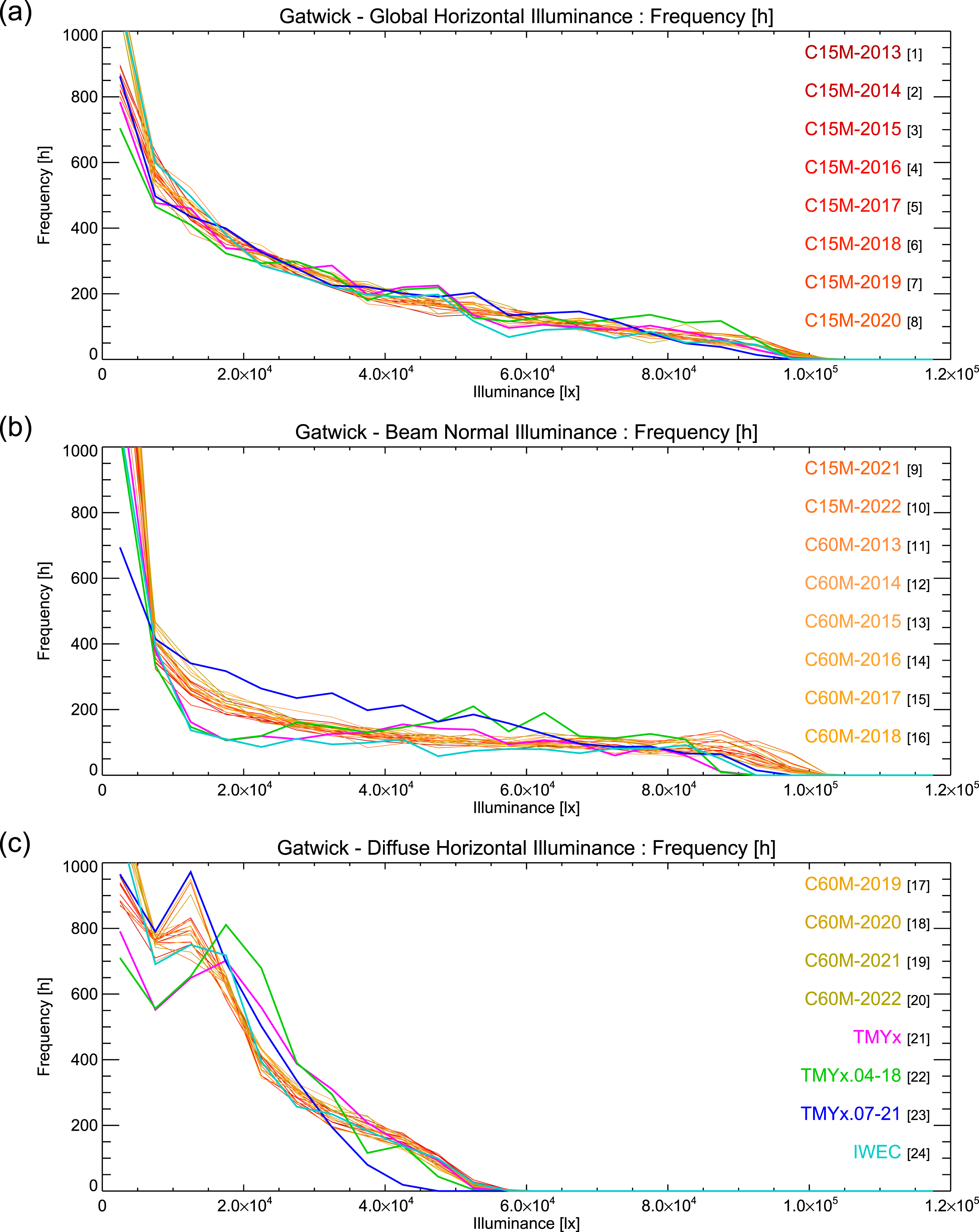

The distributions for GHI appear broadly similar for all weather files, Figure 10(a). However, it is noticeable that the CAMS AMY lines form a fairly smooth and close-knit ‘braid’, whilst the four TMY lines vary with values both above and below the AMY ‘braid’. For the CAMS data, the BNI (Figure 10(b)) has a similar shape to the GHI: there are fewer hours of high BNI. The peak BNI is approximately 10% higher for the CAMS data compared to all TMYs. The TMY and IWEC files consistently fall outside the envelope of the CAMS data. The biggest discrepancy is for the TMY 2007–2021 which has a smaller peak in low BNI (the lowest non-zero value) and then consistently has a greater frequency of higher illuminances. Distinct differences can be observed for the DHI, Figure 10(c). The general shape is similar with a smaller number of hours with a high illuminance, and a double peak at low illuminance, i.e. the first non-zero illuminance are between 1 × 10⁴ and 2 × 10⁴ lx. But there are distinct differences between the TMYs and the CAMS data. There is a clear shift in the low illuminance frequencies where the secondary peak is shifted by 5000 lx for the TMYx and TMYx 2004–2018 as well as a reduction in the peak illuminance for both TMYx and TMYx 2007–2021. Only the IWEC file sits within the envelope of the CAMS data.

Gatwick pairwise frequency comparisons for GHI, BNI and DHI

There appear to be fundamental differences between the distribution of the illuminance within TMYs and the CAMS data, but the magnitude of the differences are not obvious from inspection alone. The pairwise comparison plots provide a numerical measure for the degrees of similarity or difference between the distributions. Using equation (5), the sum of the absolute difference (SAD) between distributions was determined for all possible pairs of weather files. In other words, taking each of the 24 weather files in turn, the sum of the numerical difference with each of the other 23 weather files was computed. Thus, 24 sets of pairwise comparisons are produced. These results are presented in Figure 11. Each set of 23 pairwise values (computed using equation (5)) is presented as a column of points.

Figure 11.

GHI (a), BNI (b) and DHI (c) pairwise comparison for each Gatwick weather file with every other showing the sum of the absolute difference [h] between the frequency histogram pairs. Box is the envelope enclosing the data points for the CAMS AMYs.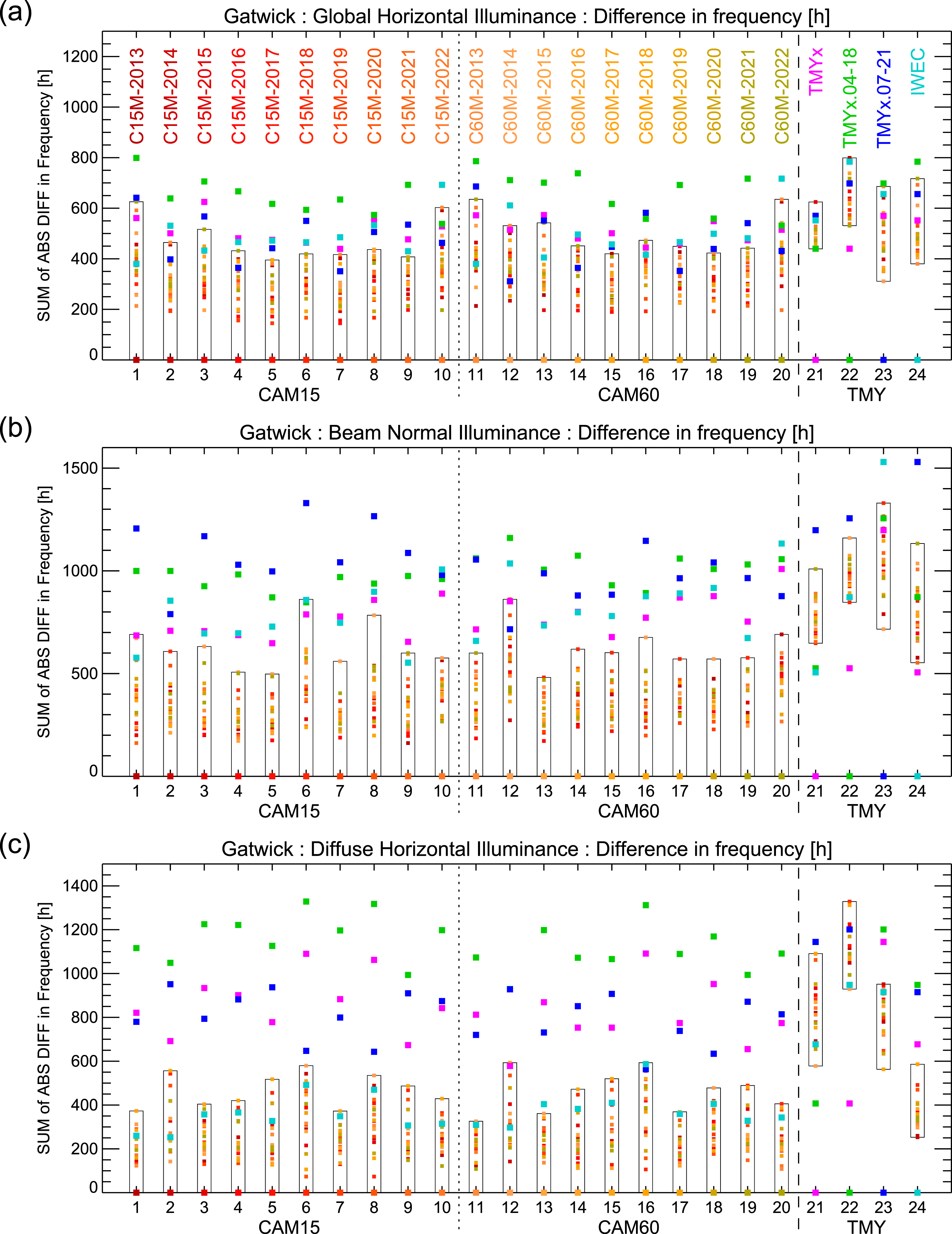

Consider the first column labelled C15M-2013 in the legend of the GHI plot (Figure 11(a)) and also ‘1’ on the abscissa for each of the three plots. The point on the abscissa is the SAD in GHI distributions between the (Gatwick) weather file C15M-2013 and itself, i.e. zero. The other points in the column give the SAD between the GHI distribution for C15M-2013 and the other 23 weather files. The points are shaded using the same colour scheme as for the frequency polygon plot. The more numerous CAMS AMY points are plotted using smaller symbols than the four TMY points. A final embellishment is an ‘envelope’ (i.e. box) enclosing the spread in the SAD for the CAMS AMY data points. Thus the envelope gives a numerical measure of the ‘tightness’ of the braid evident in the AMY distributions seen in Figure 10.

The pairwise plot presentation clearly reveals the extent to which the distributions are dissimilar. Clear differences can be seen between the CAMS data and the TMYx and IWEC weather files for GHI, BNI and DHI. However, the difference between the weather files and the CAMS data is much greater than the inter-year difference of the CAMS data. As anticipated from Figure 10, the difference between the weather files and CAMS data is greatest for BNI and DHI.

Statistic analysis such as mean absolute error, root mean square error and the coefficient of variation of the root mean square error has been used to quantify the difference between the overall distribution from the CAMS data, individual years from the CAMS data set and with the weather file illuminance data. However, the results reflect the visualisation shown by Figure 10. The magnitude of each measure is in general much larger for the weather files compared to the individual years. For example, the BNI root mean square error ranges between 3.5 × 10³ h and 6.0 × 10³ h for the weather files compared to between 0.6 × 10³ h and 4.0 × 10³ h for the CAMS years.

Gatwick magnitude polygons for GHI, BNI and DHI

Since the distributions of the illuminance from the weather files are distinct from the CAMS data, there is a need to visualise the magnitude of the difference to infer the potential impact on building design. Figure 12 shows the magnitude of the total klux hours as the sum of the frequency times the magnitude of the bin for all data for GHI, BNI and DHI (see equation (6)). The differences found in Figure 10 at low illuminance do not show up since the illuminance is too small to make a difference to the total number of klux hours. However, where the GHI looked similar in Figure 12, the differences have been amplified which shows that the total illuminance at various bins is very different to that found in the CAMS data. For example, weather file TMYx 2004-2018 has a total magnitude at bin centre 8.75 × 10⁴ lx which is 49% greater than the maximum found in the CAMS data. The TMY distributions of magnitude of BNI and DHI as measured by the total klx h are very distinct from the CAMS data. For BNI, the CAMS data peaks above 8.5 × 10⁴ lx whereas for the TMYs the highend peak is at a much lower bin. For DHI, all data sets peak at around 2 × 10⁴ lx, but the magnitudes (in klx h) are higher for the TMY files.

Figure 12.

GHI (a), BNI (b) and DHI (c) magnitude polygons for all 24 Gatwick weather files.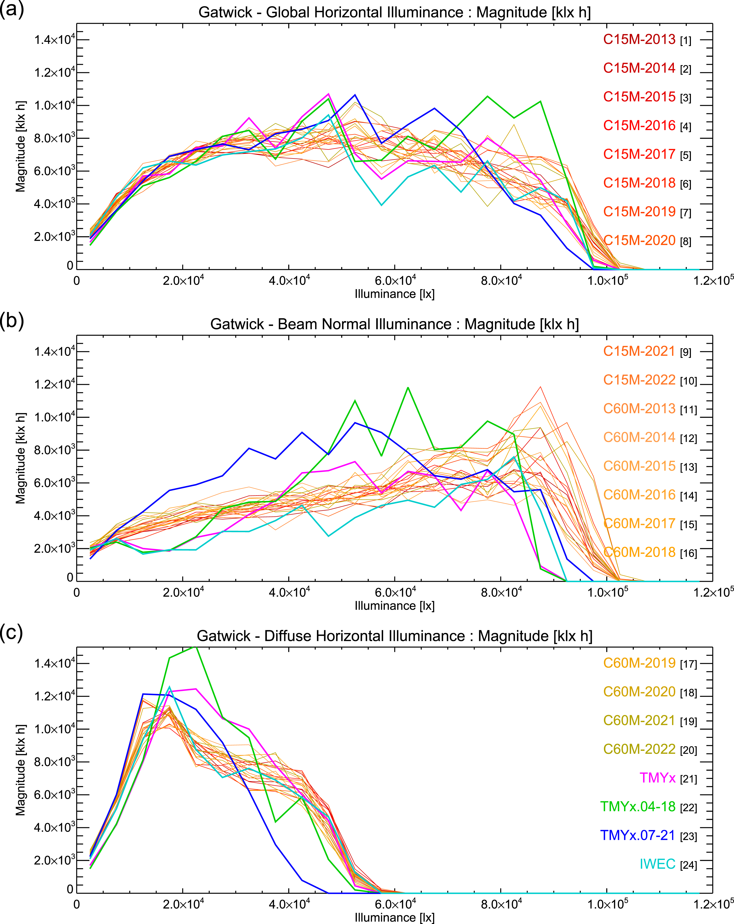

Gatwick pairwise magnitude comparisons for GHI, BNI and DHI

The pairwise magnitude comparison plots giving the difference in klux hours between the distributions for GHI, BNI and DHI are shown in Figure 13. The pattern of differences largely follows those seen in Figure 11. As before, the difference in the distributions between the CAMS and the TMY data is evident for GHI, but much more so for BNI and DHI. The distinctiveness of the CAMS distributions with respect to the TMYs is perhaps even more apparent for the magnitude than the frequency plots.

Figure 13.

GHI (a), BNI (b) and DHI (c) pairwise comparison for each Gatwick weather file with every other showing the sum of the absolute difference in magnitude between the histogram pairs. Box is the envelope enclosing the data points for the CAMS AMYs.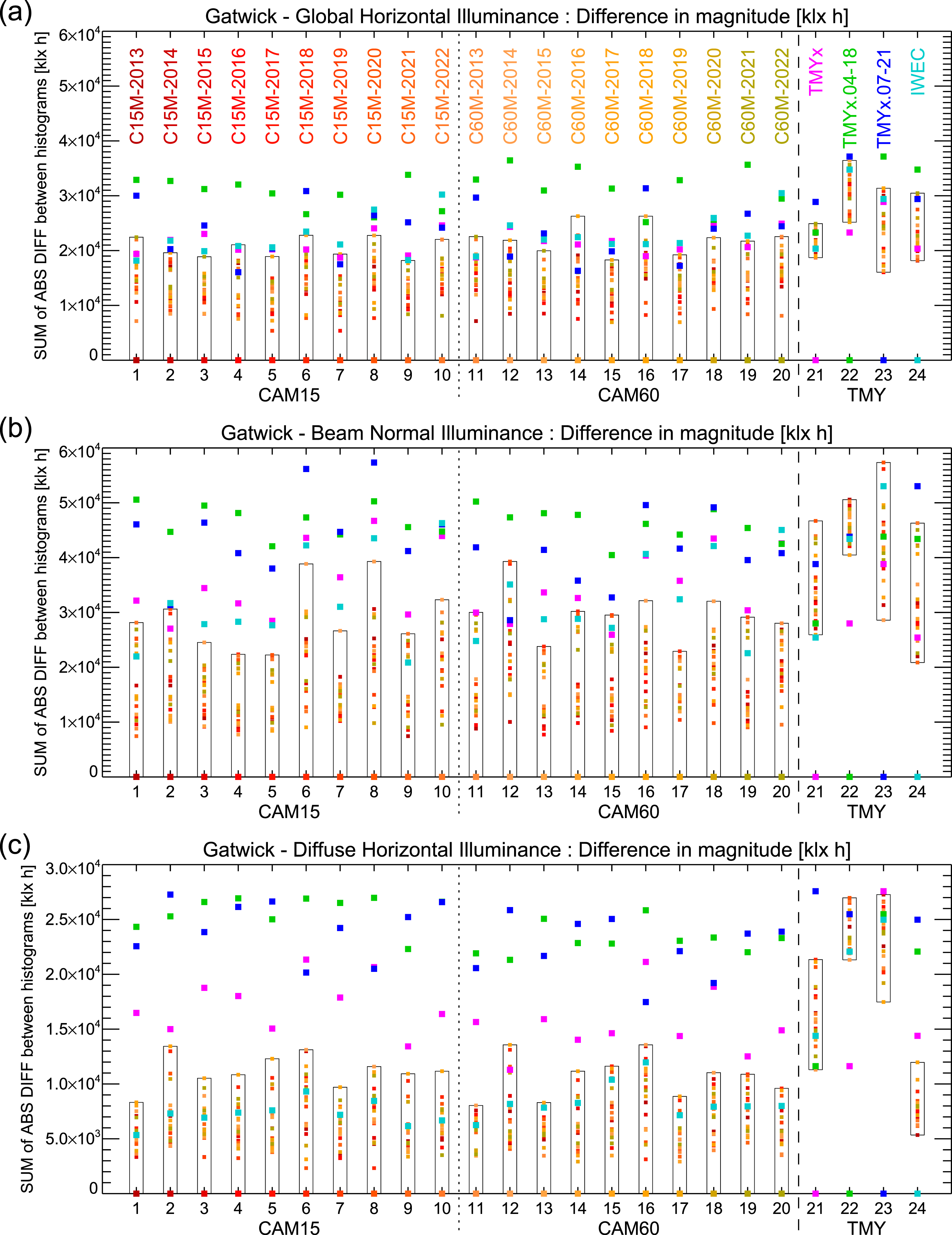

Fiumicino (Rome) and Arlanda (Stockholm) results

There are clear differences between the CAMS data and the standardised weather files for Gatwick. The authors found the degree of difference so remarkable, and thus potentially consequential for building simulation in general, that it was important to immediately expand the study to test other locations. Rome and Stockholm were chosen as locations with climates that are, respectively, sunnier and more overcast than London. The particular sites of Fiumicino and Arlanda were chosen to match the composition of the weather files used for Gatwick. Figures A1–A8 in the Appendix show the same comparisons for Fiumicino (Rome) and Arlanda (Stockholm) that were shown for Gatwick (Figures 10–13). Comparisons of the histograms show the same differences between the CAMS data and the standardised weather files for both the frequency and the magnitude plots. There are clear similarities in the GHI but the distribution of BNI and DHI follow similar shapes but have very different magnitudes and slopes suggesting very different distributions. Comparing the differences on the basis of both frequency and magnitudes, compared to all other actual years considered, shows that the standardised weather files are fundamentally following a different distribution and the differences are greatest for BNI and DHI. It is clear therefore that the findings from the Gatwick data are not a spurious outcome, and very similar findings were determined for two other locations in different countries having differing degrees of sunlight and skylight availability. For all three locations the differences between the CAMS data and the TMYs were evident in GHI, but markedly greater for BNI and DHI.

Dissimilarity matrices

With the scope of the analysis now expanded to three locations, a compact means of summarising the findings was needed. A dissimilarity matrix seemed suitable for this task. However we were not aware of this approach having been used before for the comparison of weather files, so a brief exposition precedes the presentation of the results.

In general terms, a dissimilarity matrix D describes the pairwise distinction between n objects. It is a square symmetrical n × n matrix, i.e. d _ij = d _ji . Thus the matrix is mirrored along the diagonal. The diagonal elements are usually equal to zero, i.e. the distinction between an object and itself is zero. The element d _ij is equal to the value of a chosen measure of distinction between the i-th and the j-th objects. Here, the ‘objects’ are the pairwise SADs of the distributions in GHI, BNI and DHI for the 24 weather files giving either the number of hours per bin (Figure 11) or the amount of klux hours per bin (Figure 13). Consider the plot showing the GHI number of hours per bin pairwise comparison for Gatwick (Figure 11(a)). The dissimilarity matrix (DM) which results from that pairwise plot has dimensions 24 × 24, and each element contains the numerical value from the pairwise comparison shaded using false colour. Thus the DM shows the data from each of the pairwise comparison plots as a ‘heatmap’. As noted, the points are duplicated on either side of the (mirror line) diagonal.

For the 24 weather files under evaluation, the DM comprises various regions according to the source of the data. These regions are illustrated in Figure 14. There are three main regions in the DM: a 20 × 20 region where the comparison is CAMS AMYs with CAMS AMYs; a 4 × 20 region where TMYs are compared with CAMS AMYs; and, a 4 × 4 region where the comparison is TMY with TMY. The 20 × 20 CAMS region comprises three 10 × 10 sub-regions where the comparisons are: CAM15 with CAM15; CAM60 with CAM60; and, CAM15 with CAM60. For the last of these regions, a short dashed-line diagonal marks where a CAM15 AMY is compared with a CAM60 AMY from the same year.

Figure 14.

Annotated illustration of a dissimilarity matrix.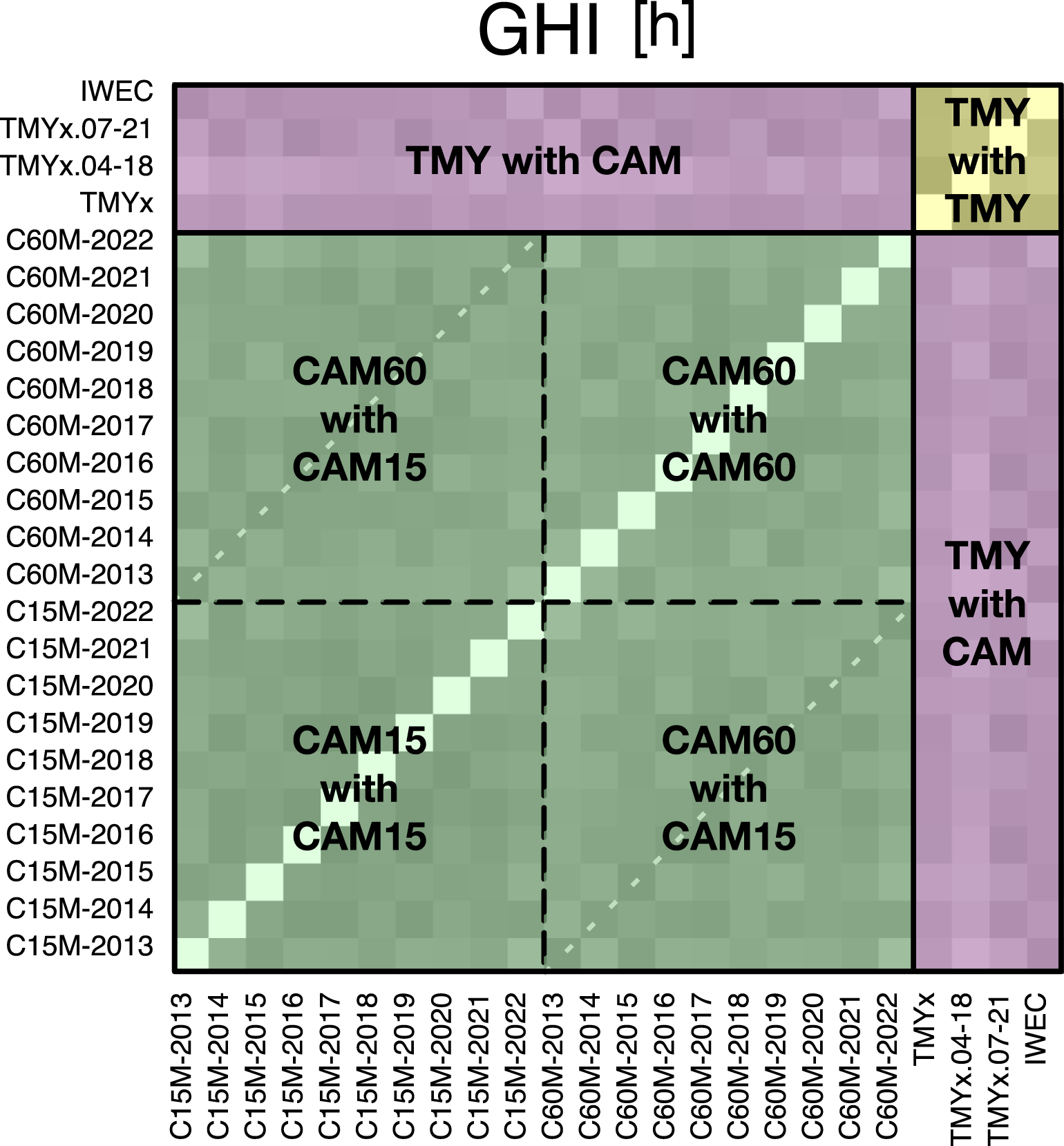

The GHI, BNI and DHI dissimilarity matrices for all three locations (Gatwick, Fiumicino and Arlanda) giving the sum of the absolute difference in hours per bin between the distributions are shown in Figure 15. To recap, the top row (a) for Gatwick shows the three DMs derived directly from the pairwise comparison data shown in Figure 11. As expected for GHI, the overall dissimilarity between the 24 weather files is less than for BNI and DHI. Nevertheless, even with GHI, pairwise comparisons with any of the four TMYs (i.e. the top four rows or the [mirror] last four columns) largely show greater dissimilarity than the comparisons within the CAMS AMY data. For BNI and DHI the dissimilarity of the TMYs with the AMYs is much more conspicuous, and the 4 rows (or mirrored 4 columns) for the TMYs stand out as markedly dissimilar to the AMYs. The exception is the (Gatwick) IWEC data for DHI which shows less dissimilarity with the AMYs than the three TMYx files. This is evident also in Figure 11(c) where the IWEC data point was the only one of the four TMYs to fall within all 20 envelopes (i.e. the differences within the CAMS AMY data).

Figure 15.

Dissimilarity frequency matrices for GHI, BNI and DHI showing the sum of the absolute difference (SAD) in hours across all pairs of distributions for Gatwick (a), Fiumicino (b) and Arlanda (c).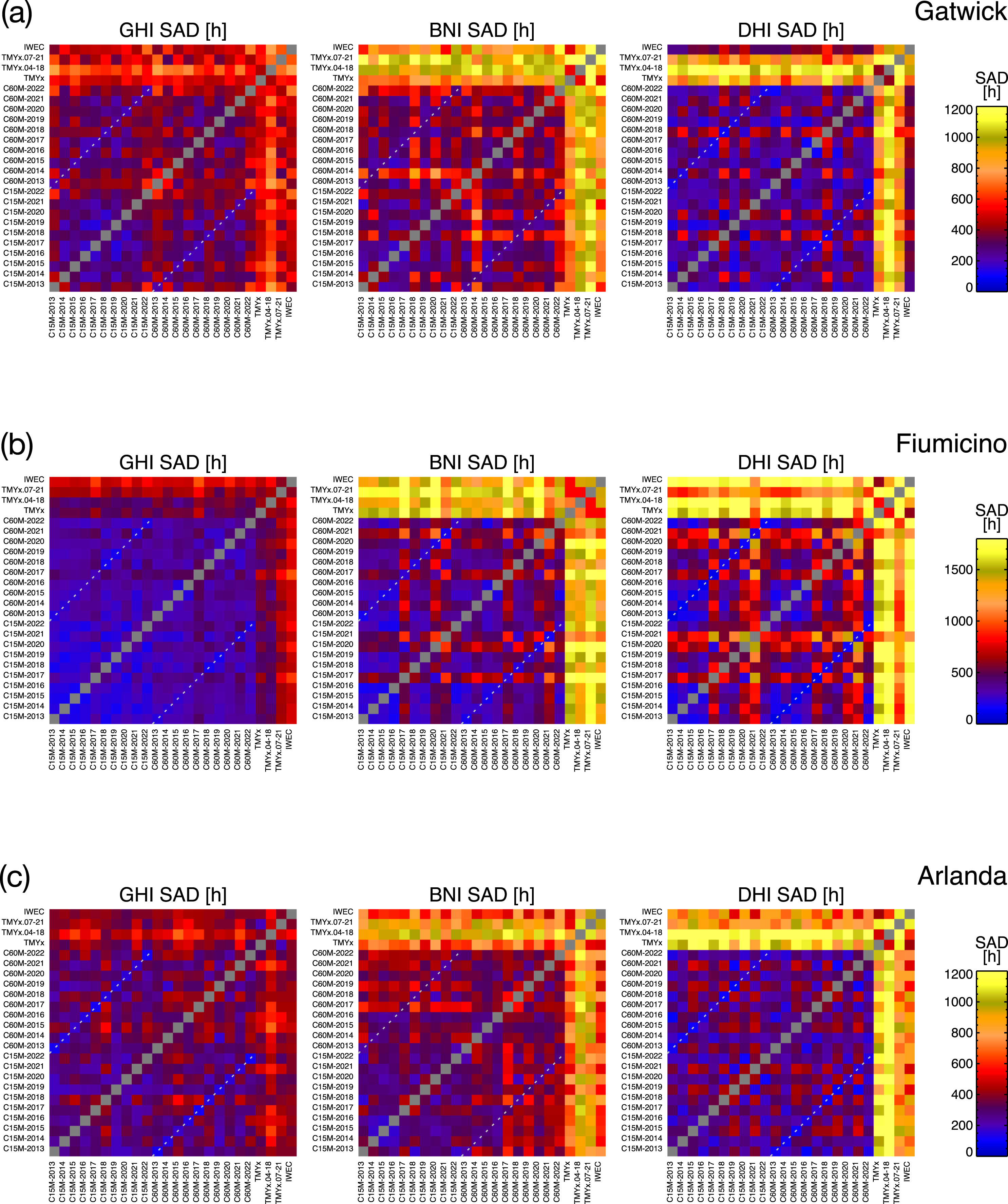

For Fiumicino (Figure 15(b)) the dissimilarity between the CAMS AMYs and the TMYs is much more pronounced, especially for BNI (note the false colour scale maximum is 1800 h). For Arlanda (Figure 15(c)) a similar pattern of dissimilarity between the TMYs and the CAMS AMYs is evident, what is perhaps notable here is that the TMY dissimilarity is greater for DHI than BNI.

Discussion

The analyses conducted in this paper call – or perhaps ‘shout’ – for more routine checks on the weather files that are used globally to design most buildings. Their applicability for representation of outdoor luminous conditions (and of solar radiation) is questioned, as comparisons of Typical against Actual Meteorological Years resulted in significantly different frequency distributions. As a consequence of these findings, we believe there is sufficient evidence to justify the case for a reassessment of weather files against historical data. This is even more important in view of the effects of climate change, which are disrupting typical climates in ways that are hard to predict and incorporate in building performance analysis. If such routine checks cannot be guaranteed, should the TMY methodology itself be placed under scrutiny and perhaps replaced by something more robust?

Of course, the analysis described here needs to be extended to include other locations. Also it is important to understand why the frequency distribution analysis appears to have uncovered differences that have hitherto gone unnoticed. The authors have considered the possibility that the frequency distribution approach is somehow too revealing of differences between, say, the TMY weather files. In other words, ‘amplifying’ differences that are in fact small. This, however, seems unlikely. Firstly, there is the marked variance in the TMY total annual illuminance values, particularly for BNI, Table 1. Next, if the approach were ‘too revealing’, it would be expected that the CAMS data would show marked variability across the ten years evaluated. Lastly, it would also be expected that whatever the inter-year variance in the CAMS data, the standardised weather files – if representative of the ‘ground truth’ – would sit within the range of the CAMS data. This was, evidently, not the case.

In addition to the analysis presented, we also used a Kolmogorov–Smirnov (K-S) test to check the likelihood of whether the TMYx and IWEC illuminance data could have been drawn from the overall distribution of the CAMS data. While the K-S test suggested that it was extremely unlikely they were sampled from the CAMS data, the same was found for some individual years from the CAMS data proving the overall comparison inconclusive. We consider this may be due to the restricted number of years in the CAMS data set used, i.e. just ten.

To recap, the authors did not expect the analysis of BNI and DHI distributions to reveal a pair of distinct populations: one fairly homogeneous consisting of ten years of satellite data (at either 15 min or 60 min), and the other comprised of four standardised weather files which exhibited much greater variance with each other than that shown between years in the AMYs. Consequently, it was not possible to address one of the original aims of the investigation: the identification of the TMY that most closely reproduced the distributions in 10 years of satellite-derived data for BNI and DHI. This led us to consider other approaches to addressing the underlying issue – how to identify and apply location-specific solar data for the CBDM evaluation of daylight standard criteria. But also the use of solar data more generally for building simulation. The following sections describe some of the ideas that resulted from these deliberations. These are presented to stimulate debate and ideas for further research to address these issues.

Multi-year AMYs as a replacement for standardised TMYs

Rather than basing the outcome of a CBDM evaluation on a single standardised file, why not use multiple AMYs from recent years? The outcome is then assessed from a profile of results, say 10 in number if a recent decade of AMYs are used. We propose that this sequence of consecutive AMYs be termed a Recent Meteorological Decade or RMD. The previous decade of AMY data can be considered to be representative of the conditions here and now, but including, of course, the inherent (i.e. ‘typical’) variability of that decade’s weather. For, say, a pass/fail compliance criterion or recommendation, the number of passes out of 10 could be thought of as a measure of the design’s resilience with regard to variation in recent weather. Thus the outcome would be based on the evaluation criterion (e.g. EN 17037 50/50 target for 300 lx) and the score out of 10 indicating how many times it has been achieved.

The multi-year RMD approach has several appealing characteristics, the foremost being:

(i) It eliminates the necessity (and uncertainty) from having to choose between the various candidate standardised TMY files.

(ii) The RMD dataset would be routinely updated on an annual basis; thus the RMD would gradually ‘absorb’ any empirical data that captures the effects of climate change. Note, the periodic updating of standardised weather files does not follow any regular schedule and is essentially carried out on an ad hoc basis.

Additionally, a profile score based on outcomes from an RMD evaluation would allow for the identification of truly exceptional AMYs. For example, a test-case design has consistently passed with a score of 10/10 for a number of years, e.g. 2010–2019, 2011–2020, etc. But, with the addition of the latest full year (say, 2023) to the test decade, the design then consistently fails for that most recent full year. This could be an exceptionally rare weather year or possibly indicative of accelerating climate change.

The case for sub-hourly weather files

Since the establishment of repositories of weather data for building simulation in the 1980s, an hourly time-step has been the accepted standard. Thus nearly all standardised TMY weather files contain 8760 rows of data (plus header information). Building simulation programs however (e.g. Energy Plus) typically operate at sub-hourly time-steps in order to accurately model energy flows, etc. Additionally, the programs can read sub-hourly weather data (usually for specialised studies) and/or output a time-series of results at sub-hourly time-steps. Sub-hourly values for, beam normal illumination (or irradiation) can be created by: interpolation of hourly data ²⁷ ; application of a stochastic generator ²⁸ ; or, some combination of the two. There is now a considerable body of research on various models to (synthetically) increase the resolution of solar and wind time series for energy system modelling. ²⁹

Rather than introducing uncertainty by using synthetic sub-hourly variation for solar radiation, the CAMS data could prove to be an empirical source of 15 min variability for BNI and, less importantly, DHI also. A 15 min time-step for solar radiation offers a significant positional improvement over an hourly increment: the sun traverses an arc of 3.75° rather than 15°. This refinement could be achieved by interpolating the hourly data to 15 min. However, this would not introduce variability in, say, BNI (as defined by equation (3)) because the 15 min interpolated points would be along the existing lines joining the 60 min data points. In contrast, the CAMS 15 min data clearly exhibit a significant component of the sub-hourly variability that is reflected in ground measurements. And thus is a more accurate representation of actually occurring variability than interpolation alone. It can be argued that 15 min solar data is in fact more ‘typical’ of actually occurring variability than 60 min data. See the illustration in Figure 16 for high variability day 0173. The daily variability is: 1018 klx h (BF5 15 min); 566 klx h (CAMS 15 min); and, 182 klx h (CAMS 60 min). If CAMS 60 min data were interpolated to 15 min, the measure of daily variability (182 klx h) would remain unchanged, despite any improvement in positional accuracy for the sun and ‘smoother’ changes in solar intensity.

Figure 16.

Illustrative comparison of 15 min and 60 min CAMS GHI with 15 min BF5 for day with high variability.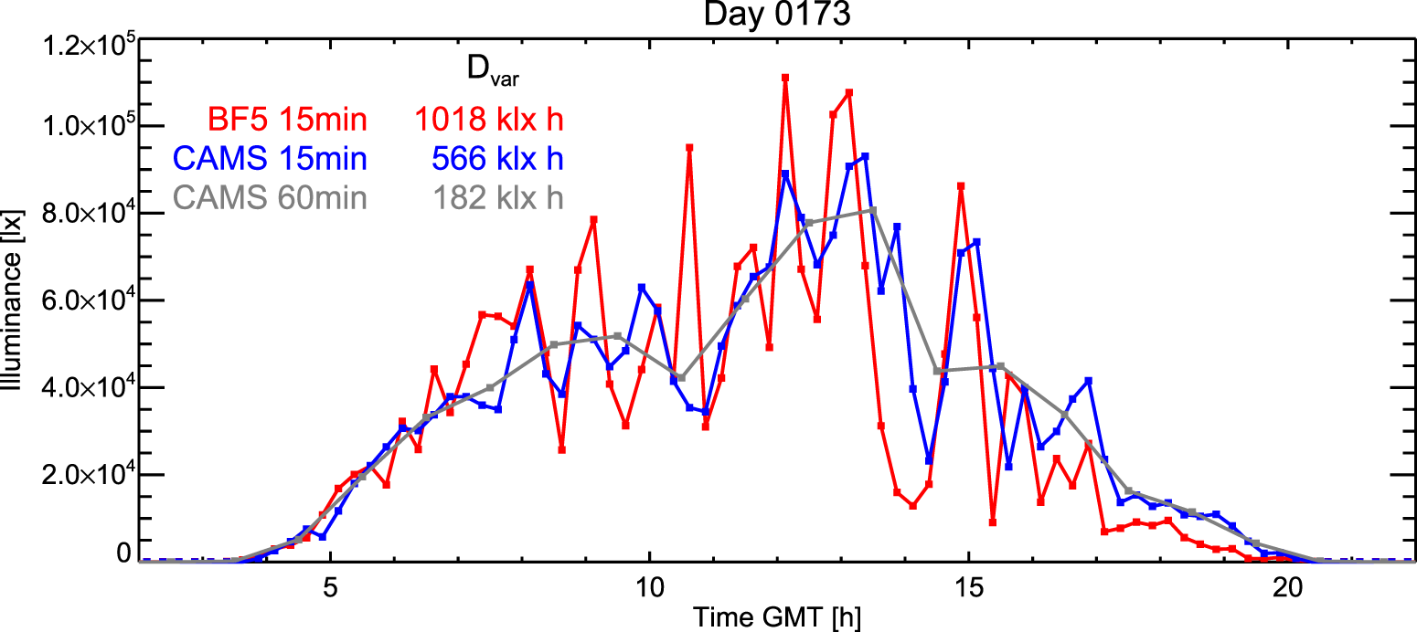

AMYs and the validation/calibration of future climate TMYs

The creation and maintenance of AMY repositories could provide a valuable means for the eventual validation and calibration of future weather files. For example, the CAMS solar data already comprises (at the time of writing) nearly two decades, with extensive geographical coverage across Europe. In 2012 Eames et al. described a set of future weather files for the epochs 2030s, 2050s and 2080s generated using a variety of means. ³⁰ The authors noted that “on an hourly basis there are clear issues with the distribution of the sunshine hours and the distribution of direct and diffuse irradiation”. In less than a decade it will be possible to test the predictions for the 2030s against satellite observations for solar radiation. Equally important, continuous long-term data (in the form of routinely updated AMYs) could provide an essential resource to support the continuous calibration/refinement of models for future weather.

AMYs and the in-situ validation of CBDM predictions

The difficulty of validating CBDM predictions under real world settings has been used to support the argument that the traditional daylight factor approach is inherently more reliable than CBDM. ³¹ Necessarily, validation of CBDM predictions requires a sufficient number of sun/sky configurations to ensure that much of the range of experienced conditions have been included in the evaluation. CBDM metrics are most often predicted for horizontal work planes, i.e. those that will generally be occupied (that is, disturbed/obstructed) by the users of the building. Thus the reliability of the measurements will be compromised by the building occupants. It is however practicable to attempt comparison of CBDM predicted internal illuminances with measured values using sensor point locations that are much less likely to be rendered unreliable than those on the horizontal, e.g. on the wall above head height. A proof-of-principle study using this approach was demonstrated by Brembilla et al. ³² The authors of that study used nearby ground measurements taken by a Delta-T SPN1 pyranometer to generate sun and sky conditions – the availability of global and diffuse horizontal irradiance time-series from a nearby weather station at Loughborough University was fortuitous. The early findings from the CAMS validation study suggest that the same quantities measured by satellite could be an equally effective resource for CBDM validation studies.

Conclusion

A validation of CAMS satellite-derived daylight data against 610 days of ground measurements for GHI has been presented. The CAMS GHI was derived from beam normal and diffuse horizontal irradiances. The evaluation was carried out in terms of: daily total GHI; 60 min and 15 min GHI; and, a comparison of daily variability calculated using the 60 min and 15 min time-series data. For all the comparisons excepting that for daily variability, the agreement between CAMS-derived GHI and that measured on the ground was very good, perhaps remarkably so. For daily variability, the CAMS and BF5 results for 60 min data were very similar. For 15 min data, CAMS could not reproduce the full degree of variability in GHI measured on the ground. However, 15 min CAMS variability was markedly greater than that exhibited by the 60 min data. More generally, CAMS was shown to be a high-quality daylight resource, with practical application for a variety of experimental purposes, e.g. post hoc retrieval of boundary daylight data for personal light exposure field studies. For the specific purpose of this article, we believe the validation is amply sufficient to justify the use of CAMS data as a basis for the evaluation of solar data in TMYs.

Satellite derived illuminance time-series of GHI, BNI and DHI for ten years (2013–2022) were compared with the same parameters from four standardised weather file sources for three locations in Europe: London (Gatwick), Rome (Fiumicino) and Stockholm (Arlanda). The evaluation was based on the difference in frequency distributions on a pairwise basis. The satellite data were sourced from the Copernicus Atmosphere Monitoring Service (CAMS). Using this approach, the ten years of CAMS data exhibited remarkably homogeneous distributions. Whereas the distributions in the TMY files were heterogeneous – differing with each other to a much greater extent than the inter-year variation seen in the CAMS data. Consequently, for all three locations it was not meaningful to attempt to identify a TMY which most closely matched the (relatively close-knit) distributions seen in the CAMS data.

The large degree of divergence between the TMY and the CAMS distributions was surprising, and certainly requires further investigation. The existing validation work on CAMS has often found it to the most reliable source of remote-sensing irradiance data. The preliminary results from the validation of CAMS-derived illuminance for GHI and DHI against ground measurements is extremely encouraging. This, together with the noted lack of agreement between CAMS and TMY distributions, suggests that AMYs derived from CAMS data could in fact offer a more reliable representation of ‘typical’ sun and sky conditions than that currently found in TMYs. And thus, potentially a more reliable basis than TMYs for the evaluation of building designs using the new daylight standards. This supposition is founded on the analysis of BNI and DHI illuminance for the purpose of CBDM. However, the findings are likely to apply equally to beam normal and diffuse horizontal irradiation, and therefore to more general building simulation, e.g. energy consumption and overheating predictions. The authors have extended the evaluation described here to irradiation and other key parameters in weather files, e.g. dry bulb temperature – that work will be reported in due course.

Supplemental Material

Supplemental Material - Daylight solar radiation AMY data derived from satellite remote sensing: Validation against ground measurements and comparison with TMYs

Supplemental Material for Daylight solar radiation AMY data derived from satellite remote sensing: Validation against ground measurements and comparison with TMYs by John Mardaljevic, Eleonora Brembilla and Matt Eames in Building Services Engineering Research & Technology