
Abstract
Summertime overheating in UK dwellings is seen as a risk to occupants' health and well-being. Dynamic thermal simulation programs are widely used to assess the overheating risk in new homes, but how accurate are the predictions? Results from two different dynamic thermal simulation programs used by four different experienced modellers are compared with measurements from a pair of traditional, semi-detached test houses. The synthetic occupancy in the test houses replicated curtain operation and the CIBSE TM59 internal heat gain profiles and internal door opening profiles. In one house, the windows were always closed and in the other they operated following the TM59 protocol. Sensors monitored the internal temperatures in five rooms and the local weather during a 21-day period in the summer of 2017. Model evaluation took place in two phases: blind and open. In the blind phase, modellers received information about the houses, the occupancy profiles and the weather conditions. In the open phase, modellers received the test house temperature measurements and, with the other modellers, adjusted their models to try and improve predictions. The data provided to modellers is openly available as supplementary information to this paper. In both phases, during warm weather, the models consistently predicted higher peak temperatures and larger diurnal swings than were measured. The models' predicted hours of overheating were compared with the measured hours using the CIBSE static threshold of 26℃ for bedrooms and the BSEN15251 Category II threshold for living rooms. The models developed in each phase were also used to predict the annual hours of overheating using the CIBSE TM59 procedure. The inter-model variation was quantified as the Simulation Resolution. For these houses, the blind phase models produced Simulation Resolution values of approximately 3% ± 3 percentage points for TM59 Criterion A and 1% ± 1 percentage point for TM59 Criterion B. The Simulation Resolution concept offers a valuable aid to modellers when assessing the compliance of dwellings with the TM59 overheating criteria. Further work to produce Simulation Resolution values for different dwelling archetypes and weather conditions is recommended.
Introduction
Summertime overheating in dwellings across the UK has been demonstrated.1–3 Reducing the risk of overheating is important due to the health implications of high indoor temperatures,4–6 and the increase in electricity demand if more air conditioning is used.7–9 As the recent UK Environmental Audit Select Committee notes, ‘The Committee on Climate Change has repeatedly recommended a standard or building regulation to prevent overheating in new buildings, however thermal comfort is still not addressed in the building regulations’.10,a The Committee points to dynamic thermal simulation (DTS) programs and CIBSE Technical Memoranda TM52 11 and TM5912,b as potential enablers of such regulation. 10
DTS programs are the obvious and, in most circumstances, the only, viable approach to assess overheating risk in homes and other buildings. Such studies are routinely undertaken by consultants and have been frequently reported in the literature (e.g.13–18). To be viable for demonstrating regulatory compliance, however, DTS programs need to steer designers towards low risk designs by correctly predicting the relative overheating experienced by alternative design proposals. This paper firstly examines the differences between models' predictions of summertime temperatures and temperatures measured in two test houses, i.e. empirical validation. Secondly, it examines the predicted differences in overheating using the test houses as a case study, i.e. inter-model comparison.
Formative research into the reliability of DTS programs19,20 has classified the errors that cause inter-model prediction variability as either external, e.g. differences in the data input to models and the way that modellers use the programs, or internal, which are embedded in the algorithms and sub-models in DTS programs. Recently, for example, Strachan et al. 21 observed significant user errors in a large multi-modeller exercise. In empirical validation exercises, differences may also exist between the actual building and the data fed into programs; a further source of external error and one that is very hard, if not impossible to remove when a validation exercise is based on measurements in real occupied buildings.
The prediction of overheating risk is especially difficult for DTS programs because it relies on accurate modelling of the highly dynamic interactions between thermal mass, air flow (i.e. ventilation) and solar radiation and other heat gains. It is precisely when these thermo-physical interactions are most pronounced, i.e. on hot sunny days when natural ventilation cooling is used, that reliable predictions are most needed. For example, in inter-model comparison work where, as far as possible, all external errors were removed, it was shown that quite small differences in daily peak temperature prediction (ca. 2℃) could amplify into differences in the predicted hours above an overheating threshold that differed by a factor of 2.5 (250%).20,c The concept of Simulation Resolution (SR) was used to quantify the inter-program variability in predictions. 22 The predictions were shown to be especially sensitive to the internal surface heat transfer algorithms used in the programs; 22 a point reiterated recently in the work of Petrou et al. 23 Elsewhere, Mourkos et al. 24 report that two models were ‘consistent’ in the prediction of overheating hours in contrast to Petrou et al. 25 who reported different overheating risks from different programs.
In an International Energy Agency (IEA) empirical validation exercise involving 17 DTS programs, run by 20 practitioners, from 11 countries, 26 it was shown that, after stringent efforts to remove all external errors, the peak temperature predictions still differed by up to 6 K (from 27 to 33℃ around a measured value of 31℃). d The study also showed that the programs differed in their assessment of whether one test cell was more or less likely to overheat than another. From a methodological perspective, the IEA study participants were unanimous in recommending that, in empirical validation work, a first phase should be conducted blind, i.e. without knowledge of the actual measurements, with a second phase being open, i.e. with the measured data available. A similar approach was used in the IEA Annex 58 validation work (e.g. Strachan et al. 21 ). More recently, Symonds et al. 27 reported similar discrepancies between simulation results and measurements in relation to overheating in 823 English dwellings, and Simson et al. 28 attribute greater-than-measured overheating predicted by programs to differences in the way they modelled heat dissipation between zones and through cross-ventilation.
Together, these studies sound a note of caution with regard to the reliability of DTS programs for overheating prediction. However, results can be very case specific, and it is the performance of contemporary DTS programs, when used by experienced modellers, which is of particular interest – especially when the programs are applied to real, typical UK homes, exposed to warm summer conditions with real, or pseudo-real, occupants, following behaviours specified in, for example, TM59.
Against this background, this paper reports the results of a collaborative study between four energy consultants and a monitoring and validation team. The consultants were keen to understand how well predictions compared to reality and to the predictions of other programs. They used two different DTS programs to predict the indoor temperatures, and thus the extent of overheating, in five rooms of two adjacent, nominally identical, semi-detached houses in the English Midlands. The rooms had ‘synthetic occupants’ to produce the TM59 internal heat gain profiles and the TM59 window and door opening profiles. Of the three sets of side-by-side experiments, the measurements made in the 21-day period during which overheating occurred are the subject of this paper. In this period, one house had operable windows and in the other the windows were closed, e in both curtains and blinds were closed at night.
Predictions were made ‘blind’ and then ‘open’ with knowledge of the measurements and other modellers’ predictions. In both phases, two types of predictions were made: Type 1, predictions of hourly temperatures during the experiments, and the hours over the CIBSE static overheating threshold of 26℃ for bedrooms 29 and the BSEN15251 Cat. II 30 threshold for living spaces, were compared with the corresponding measured values; and Type 2, predictions of the annual overheating risk, made using a standard CIBSE Design Summer Year (DSY1). The inter-model differences in these predictions are quantified using the SR concept.
Description of the test houses and measurements
House description
The measurements were made in a pair of adjoining, three-bedroom, semi-detached houses, built in the 1930s, and located in a suburban residential area of Loughborough in the East Midlands region of UK. The houses have been described in a number of previous publications.31–33
The houses have the same geometry, construction, window configuration and central heating systems,
f
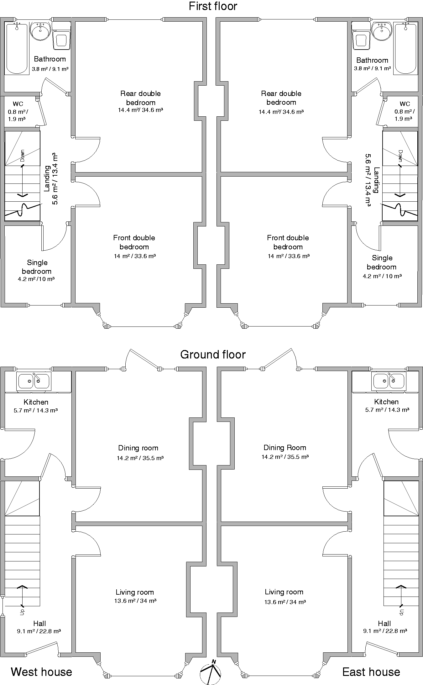
while the room layout is mirrored about the party wall (Figures 1 and 2). The front facade faced (almost) due south (Figure 2). On the ground floor, there is a south-facing living room with a bay window, a similar sized, north-facing dining room and a separate kitchen. On the first floor, at the front (south), there is a small single bedroom and a larger double bedroom with a bay window. A similar-sized double bedroom is at the rear (north). The small east and west facing windows were covered with insulating board to preclude unmatched heat losses and solar gains.
Loughborough matched pair test houses viewed from the front (a) and rear (b). The front doors face south (a). The left house in photograph (a) is the West house and the right the East house. Loughborough matched pair test houses: floor plans and dimensions to internal walls.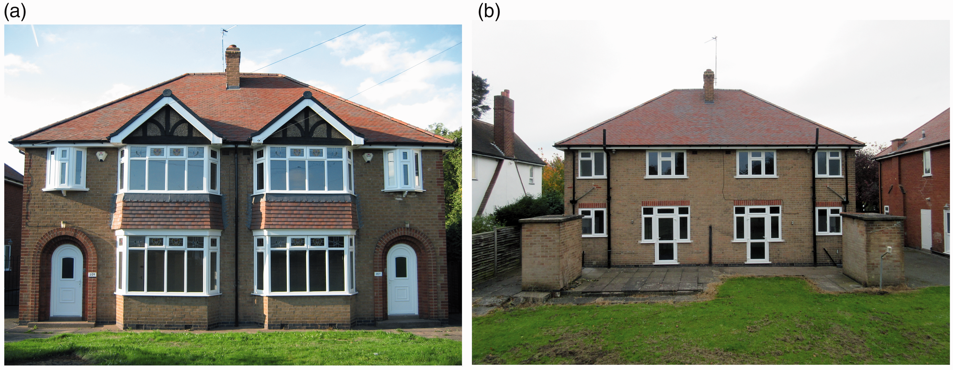
The houses' geometry was measured using calibrated laser measurement with multiple readings being taken. Some geometry was assumed, based on earlier assumptions, 34 where access was not possible, notably the depth of the floor voids. The cavity in the party wall between the houses was inspected using a borescope, although it was not possible to tell if the top of the cavity was sealed to inhibit cavity air flow.
The houses had the same uninsulated cavity wall construction, a raised wooden ground floor with a ventilated void below and ventilated roof space (loft). Both houses had recently been retrofitted with 300 mm of insulation above the first floor ceiling and double glazing to all doors and windows, which had identical operable elements. Being at least 80 years old, the houses' fabric may have deteriorated, and the condition in non-visible areas is unknown. The dwellings' fabric was therefore described by the materials and layer thickness. The thickness of the kitchen floor slab could not be determined, so was estimated as 100 mm thick based on assumptions. 34 The frame and window specifications for the double glazed windows and doors installed in 2016 were known.
The whole house infiltration rate was known from multiple blower door tests undertaken by the monitoring team. 33 The measured whole house air permeability at a pressure of 50 Pa (q50) and the corresponding air change rate (n50) were 14.7 m3/h m2 and 15.3/h, respectively, in the West house, and 14.9 m3/h m2 and 15.6/h in the East house. The air flows through the ventilated roof space, below the raised floor and through open windows were unknown.
The overall heat transfer coefficient (HTC) of each house was measured via co-heating test following the method of Johnston et al. 35 Very similar values and were recorded for the two houses: West house 223 W/K and East house 216 W/K. 33
Monitoring
Measurement of the weather conditions, synthetic occupancy and room temperatures.
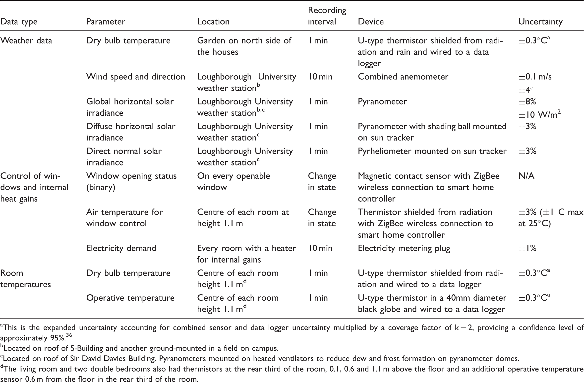
This is the expanded uncertainty accounting for combined sensor and data logger uncertainty multiplied by a coverage factor of k = 2, providing a confidence level of approximately 95%. 36
Located on roof of S-Building and another ground-mounted in a field on campus.
Located on roof of Sir David Davies Building. Pyranometers mounted on heated ventilators to reduce dew and frost formation on pyranometer domes.
The living room and two double bedrooms also had thermistors at the rear third of the room, 0.1, 0.6 and 1.1 m above the floor and an additional operative temperature sensor 0.6 m from the floor in the rear third of the room.
To ensure that the desired synthetic occupancy heat gains were being produced, the electricity demand of the electric heaters in every room was recorded with plug load meters. The status of each window, i.e. open or closed, was recorded by a contact sensor whenever a change in state occurred. Video cameras enabled the status of doors, and curtains and blinds to be checked remotely.
The indoor air and operative temperatures were measured at one-minute intervals using best practice, with air temperature sensors shielded from solar radiation and 40 mm black globe sensors for operative temperature g positioned out of direct sunlight. 33 Air and operative temperatures were measured at 1.1 m from floor at the centre of each room. To assess the spatial variation of room temperatures, additional air temperatures were measured at 0.1, 0.6 and 1.1 m from the floor and operative temperature 0.6 m from floor in the living rooms and both the front and rear double bedrooms at the rear third of the room, furthest from windows. The air temperatures at 0.6 and 1.1 m differed by less than 0.1 K, with values up to 1 K lower being recorded at 0.1 m indicating some stratification. Operative temperatures measured in the centre of the room at 1.1 m from floor and rear third of the room at 0.6 m differed by only 0.2 K.
The synthetic occupancy
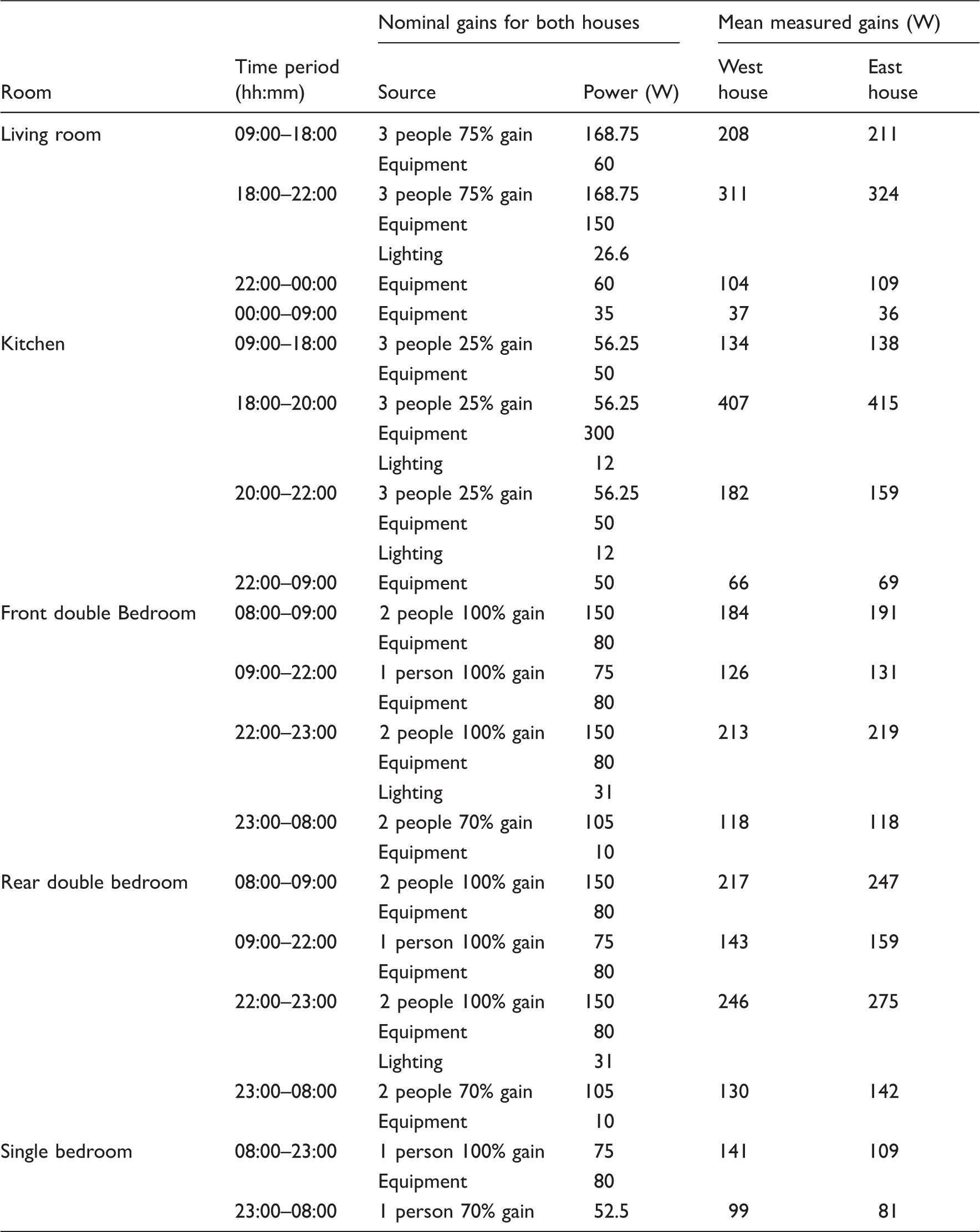
In all the experiments undertaken in the test houses, the heat gain profile in each room and the door, window and shading (i.e. curtain and blind) schedules was, wherever possible, set to mimic those recommended in CIBSE TM59. The internal heat gain profile and the internal door operating schedules were the same in both houses for all the experiments. The schedule of windows and shading operation differed between the houses depending on the experiment being undertaken.
Heat gain profiles: nominal TM59 values and actual measured values for each room.
The small top-hung windows i in the rooms were operated differently depending on the experiment, but they were either fully open or completely closed, never partially open. In rooms with more than one operable window (the living room and front bedroom), all windows were opened or closed at the same time. In the experiment where the windows were opened, they were controlled to open when the room was occupied, and the dry-bulb air temperature in the room exceeded 22℃, as defined in TM59. All rooms had the potential for window opening, except for the bathroom and dining room which were never occupied according to TM59. The windows were operated by chain actuators in response to signals from a wireless thermistor in the same room and took less than one minute to open or close. To ensure that the windows were operating correctly, their status was logged using a contact sensor reporting to an online database with room sensor temperature also being recorded. The trickle vents were closed in all tests, and there was no mechanical ventilation at any time in either house.
The curtains in the living room, dining room and bedrooms and the blinds in the kitchen and bathroom were automatically opened or closed depending on the experiment. Curtains and blinds took less than 10 s to open or close. Bedroom doors were operated by chain actuators and were closed from 23:00 to 08:00 and open at all other times in accordance with TM59 schedules. All other internal doors were always open.
The test house experiments
The experiments: timing, duration and window/shading schedules.
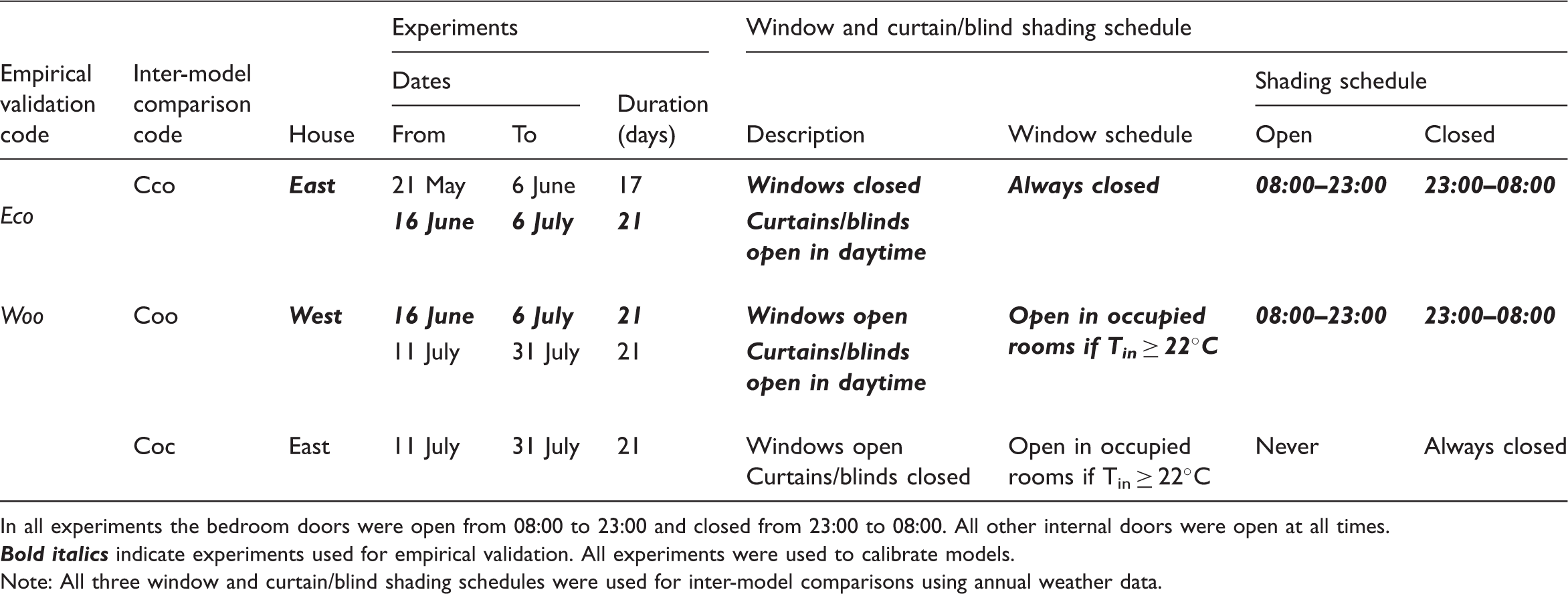
In all experiments the bedroom doors were open from 08:00 to 23:00 and closed from 23:00 to 08:00. All other internal doors were open at all times.
Comparisons between measurements and predictions were made for all three experimental periods. However, this paper focuses on the second experimental period, from 16 June to 6 July 2017. During this period, there was a spell of hot weather which caused overheating and thus stressed the reliability of the models for making accurate predictions of overheating risk. Both operative and air temperature were measured in the test houses and predicted by models, but only operative temperature is analysed in this paper because it is the most commonly used temperature metric in overheating assessment.
The chosen 21-day experimental period also enables a direct, side-by-side, comparison of the measured and predicted influence on overheating of having windows either permanently closed or operable. In the East house, windows were always closed, and the blinds and curtains were open from 08:00 to 23:00 and closed from 23:00 to 08:00, in accordance with TM59 sleeping schedule (Experiment Eco j ). In the West house, the blind and curtain schedule was the same, but the windows were opened if the room air temperature exceeded 22℃ and it was occupied (according to the TM59 occupancy profiles, Table 2) and closed if the air temperature fell below 22℃ or the room became unoccupied (Experiment Woo k ).
Assessing the DTS programs
The programs, modellers and predictions
Four highly skilled modellers carried out the modelling. They were all employed in professional organisations and had relevant professional experience ranging from 8 to 20 years. None were involved in the experimental work or had prior knowledge or experience of the test houses.
Modeller code, program code and program version.
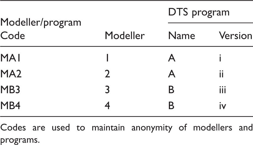
Codes are used to maintain anonymity of modellers and programs.
Following the recommendations from previous empirical model validation exercises,21,26 predictions were first made ‘blind’, i.e. without knowing the temperatures measured in the houses. Thereafter, in an ‘open’ phase, the measured room temperatures and the blind phase predictions of all four models/modellers were revealed. The initial blind phase more closely resembles the situation encountered by modellers who are making overheating risk assessments of new l or existing buildings.
Modellers were asked to make two types of prediction in each phase:
Type 1: Predictions of the hourly room temperature
m
using the measured internal heat gains and the measured weather for experiments Eco and Woo (Table 3). Type 2: Predictions of the annual incidence of overheating for three window opening and shading schedules (Cco,
n
Coo
o
and Coc
p
) using annual DSY1 weather data for the location and TM59 overheating Criteria A and B (Table 3).
Type 1 predictions enable comparisons between hourly averaged measurements and hourly predicted temperatures in each of the five rooms, the living room and kitchen downstairs and the front bedroom single bedroom and rear bedroom upstairs. The comparisons were made using temperature against time plots as well as by deriving standard metrics to quantify the differences (errors) between the two: mean error, 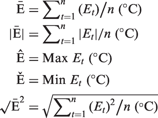

It was also possible to compare the measured and predicted hours for which the bedroom temperatures exceeded the static CIBSE threshold of 26℃ during the synthetic sleeping hours, 23:00–08:00: 189 h total for each 21-day experiment. Also compared were the measured and predicted hours for which the living room and kitchen exceeded the BSEN15251 thermal comfort threshold during the synthetically occupied hours, 09:00–22:00: 273 hours total.
BSEN15251
30
is an adaptive comfort threshold derived from the exponentially weighted running mean of outdoor air temperature (Trm). Category factors are applied to comfort thresholds based on the building type and assumed occupant vulnerability level. As the test houses had been recently renovated, the Category II threshold (±3 K) was selected as this is appropriate for adults of normal thermal expectations in new or renovated dwellings. Overheating was determined by counting the number of hours above the Category II upper comfort threshold (Tupp), where

The Type 2 predictions enable an inter-model comparison of the predicted hours over the TM59 threshold temperatures and a comparison of whether or not the predictions provide a similar assessment of overheating risk as judged by the TM59 Criteria. 12 Criterion A, which applies to living rooms and bedrooms during occupied hours, is based on the adaptive overheating assessment method outlined in CIBSE TM52, 11 which is based on the BSEN15251 adaptive comfort standard. 30
For each hour between 09:00 and 22:00 in living spaces
r
and all hours in the day for bedrooms, the difference between the predicted operative temperature (Top) and the Category II upper temperature threshold (Tupp) is calculated to derive ΔT, which is rounded to the nearest whole degree

The number of hours where ΔT ≥ 1℃ between May and September is then calculated. Criterion A is failed if the number of hours is more than 3% of the occupied hours between May and September: 1989 h for living spaces and 3672 h in bedrooms.
Criterion B is a static comfort criterion applicable to bedrooms only. The number of annual hours for which the predicted bedroom operative temperature exceeds 26℃ between 22:00 and 07:00 is calculated. Criterion B is failed if the number of such hours exceeds 1% of annual hours between 22:00 and 07:00, which is 3285 h. s
The blind phase
In the blind phase, the four modellers were provided with: a description of the test houses; the overall measured infiltration rates and HTCs; the synthetic occupancy profiles and the window, door and shading schedules; the weather data and information already published about the houses.31–34,39 Other than these data, the modellers were given complete freedom to model the dwellings as they chose. Each modeller was aware that others were involved in the project but did not confer. The experimental team acted as an information point and if a question was posed by one modeller, the question and the answer were provided to all other modellers. This ensured that, at all times, all four modellers had the same information.
Two weather files were provided to each modeller in the format required by their own DTS program. The first contained the hourly outdoor dry-bulb temperatures, solar radiation and wind data as measured between 21 May and 31 July 2017 (see ‘Monitoring’ section). They thus had the data and house descriptions necessary to precondition the model prior to making predictions. The second weather file was the CIBSE DSY1 file for the 2020s, high emissions, 50% percentile scenario, for Nottingham, which is 23 km north of the test houses.
The modellers were also provided with a document that detailed the houses' geometry, construction and occupancy profiles. Geometry included: site location, orientation and plan; the house plans, elevations and surroundings; roof overhangs and shading; ceiling heights on each floor; internal and external door dimensions; window reveal and sill dimensions and window frame and opening geometry. The construction details included: material layers and thickness; glazing thermal and solar transmission properties; curtain and blind fabric solar transmission properties and subfloor airbrick sizes and locations.
The thermal conductivity (and density) of the materials used in the construction of the test houses was not known, and modellers were encouraged to use whichever values they felt appropriate based on look-up tables within their simulation tool, their personal experience or other references. t Modellers also had to calculate glazing ratios based on the window and frame geometry provided.
Blind stage U-values calculated from the construction layers used by modellers.
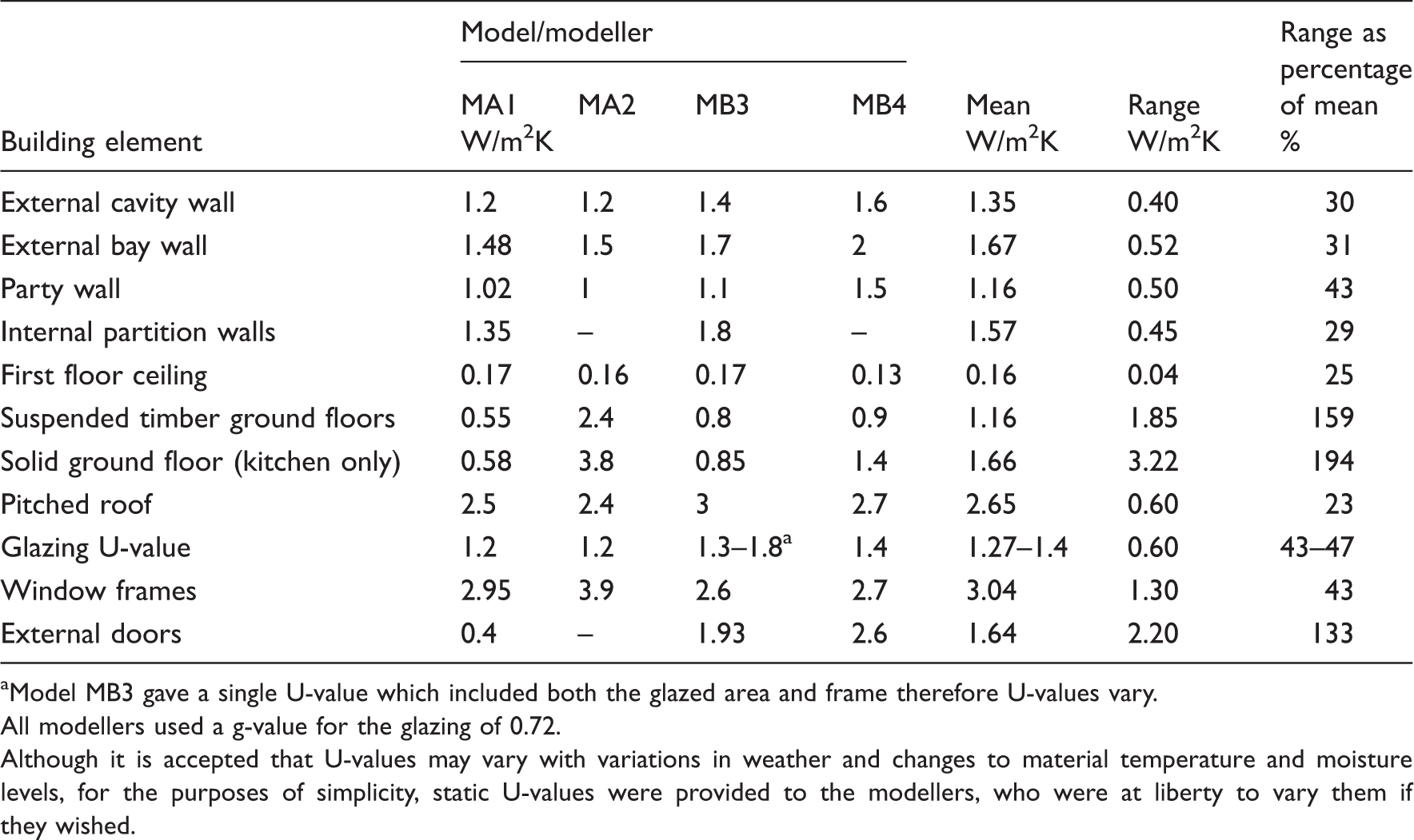
Model MB3 gave a single U-value which included both the glazed area and frame therefore U-values vary.
All modellers used a g-value for the glazing of 0.72.
Although it is accepted that U-values may vary with variations in weather and changes to material temperature and moisture levels, for the purposes of simplicity, static U-values were provided to the modellers, who were at liberty to vary them if they wished.
The infiltration rate of the houses is perhaps the most significant source of uncertainty. Although the ventilation rates in the roof space and below the raised floor were unknown, the modellers were provided with a whole house value of air leakage, q50, and ventilation rate, n50, as calculated from the blower door tests (‘House description’ section). To derive a value for the infiltration rate at ambient pressure, all the modellers converted q50 into an equivalent whole-house air change rate at ambient pressure using the conventional K–P model approach of dividing by 20 (e.g.40,41). This approach has been shown to be rather approximate 42 with divisors of 10–30 showing better results depending on the building in question. 43 Furthermore, at any given instant, the actual infiltration rate will depend on wind pressures and indoor to outdoor temperature differences; as summertime tracer gas decay measurements made in the test houses have shown. Some models modulate infiltration with external wind speed to account for this variability. The sensitivity of models’ predictions to the infiltration rates was explored by the modellers in the open phase.
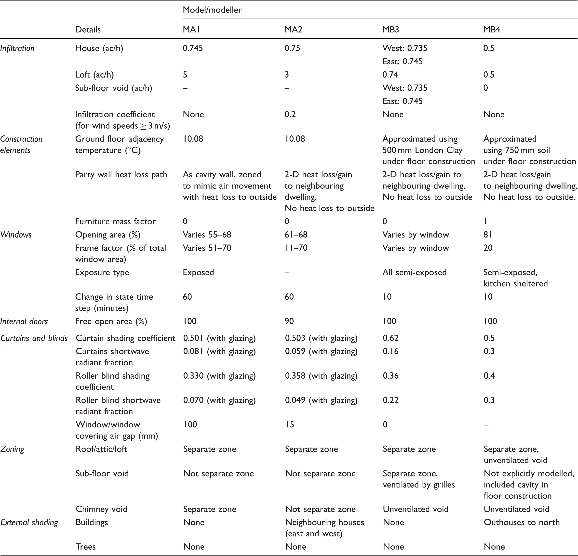
Blind stage assumed and calculated model inputs for each modeller.
The open phase
The open phase comprised two one-day workshops where the modellers were encouraged to openly compare their models and assumptions with each other and to consider the relationship between their DTS program's predictions and the measurements. The modellers undertook sensitivity analyses to see which, if any, of the parameters used by the programs contributed to the difference between the measured and modelled results.
The modellers suspected that the main source of difference between the models and the measurements was: the infiltration rate, solar gains, fabric U-values and the internal thermal mass. They therefore undertook sensitivity analyses to explore the effect of variations in these factors on their programs' predictions. They also corrected simple input errors made in the blind phase. The modellers returned their open phase predictions within two weeks of the second workshop.
Open phase adjustments made by each modeller.
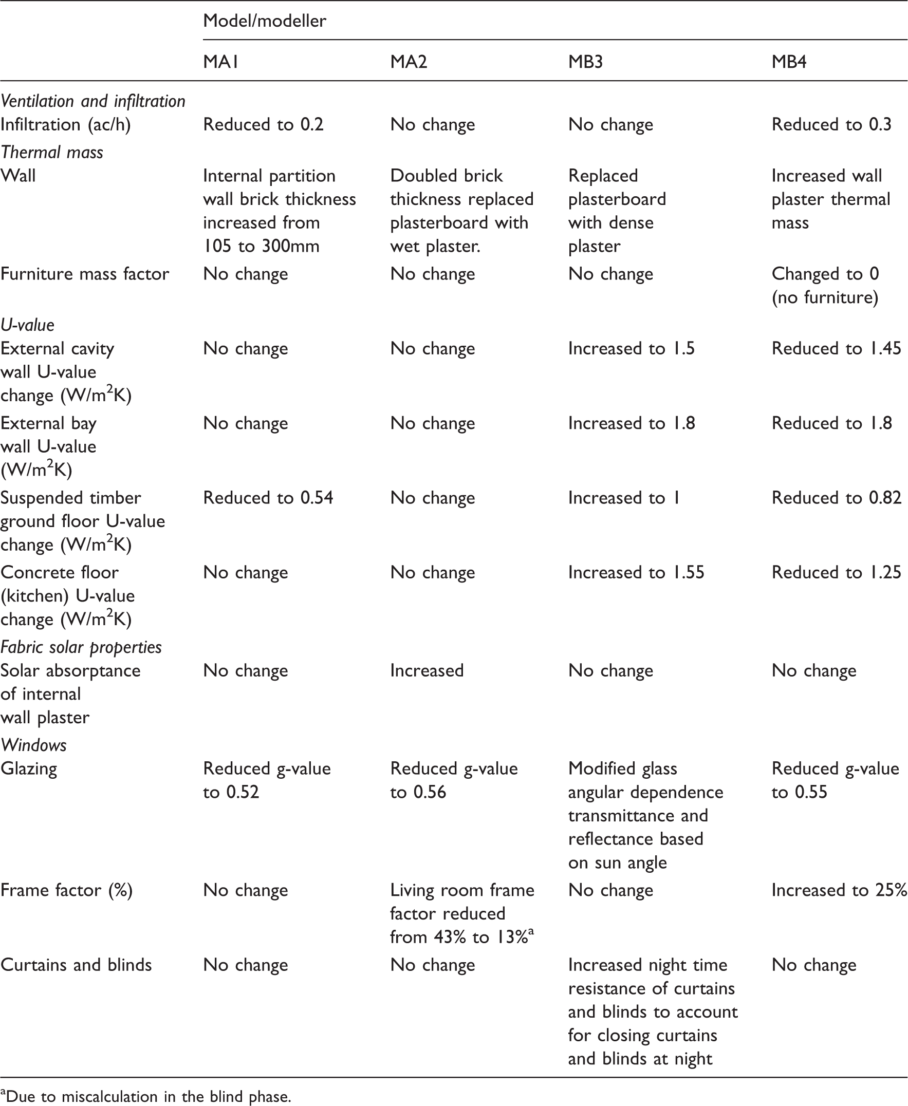
aDue to miscalculation in the blind phase.
The impact of infiltration rate was also investigated with modellers varying the value between 0 and 4 ach to try and understand the effect on the absolute predicted temperatures and the diurnal swings in temperature. w Interestingly, the changes altered the absolute temperatures but not necessarily the diurnal temperature swing. Ultimately two modellers made only small changes to the infiltration rates used in the blind phase.
Overheating is often driven by solar radiation, and so the reliability of the weather station solar data was examined. To this end, the experimental team supplied modellers with two further weather data sets that were recorded within 500 m of the original weather data at Loughborough University; using these data, there was negligible difference in the model predictions. x It was concluded that any uncertainty in the weather data was not a significant cause of uncertainty in model predictions.
The g-value assumed for the windows was revisited by the modellers and found, not surprisingly to have a noticeable impact on the predicted internal room temperatures on sunny days. Consequently, three of the modellers reduced the g-value of 0.72, which was used in the blind phase, by between 22 and 28%.
Changes to fabric U-values also directly affected the predicted peak room temperatures, with lower U-values causing higher daily peaks. The modellers using program A made limited or no changes to the fabric U-values, whereas those using program B did adjust the assumed U-values.
At the open phase workshop, infrared photographs of the houses were also examined after one modeller suspected that air was being drawn through the cavity from the air bricks at the bottom, up the cavity and either into the roof or out of the air brick at the top. Cavity wall ventilation represents a source of modelling uncertainty that might not be present in modern dwellings.
Results: Comparisons between predictions and measurements and between the predictions of the different models
Empirical validation: Comparison of measurements and predictions
Analysis of the measured results focuses on the period from 16 June to 6 July 2017. Between 17 and 21 June, there was a five-day warm spell during which the outdoor temperature reached an hourly peak temperature of 29.7℃ on 18 June with a peak global solar irradiance of 936 W/m2 on 5 July. The final day of the experimental period, 6 July, was also warm. Between these dates, the outdoor temperature rarely exceeded 21℃ (e.g. Figure 3(e)).
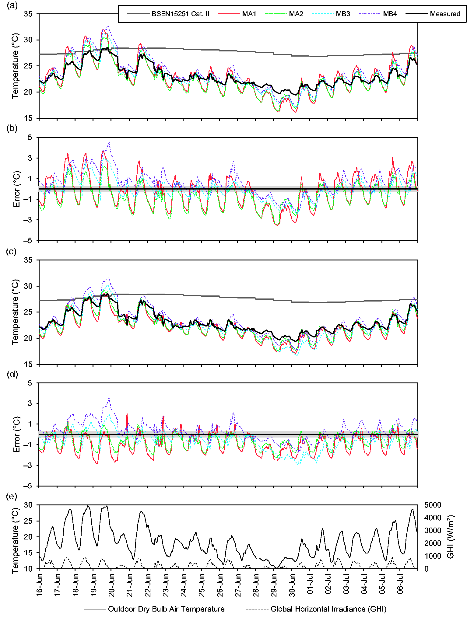
Experiment Eco: operative temperatures measured in the living room and the temperatures predicted by each model: (a) measured and predicted, blind phase; (b) difference between measured and predicted, blind phase; (c) measured and predicted, open phase; (d) difference between measured and predicted, open phase; (e) outdoor air temperature and global horizontal irradiance. Grey shading around measurements on plots b and d indicate 0.3℃ measurement uncertainty.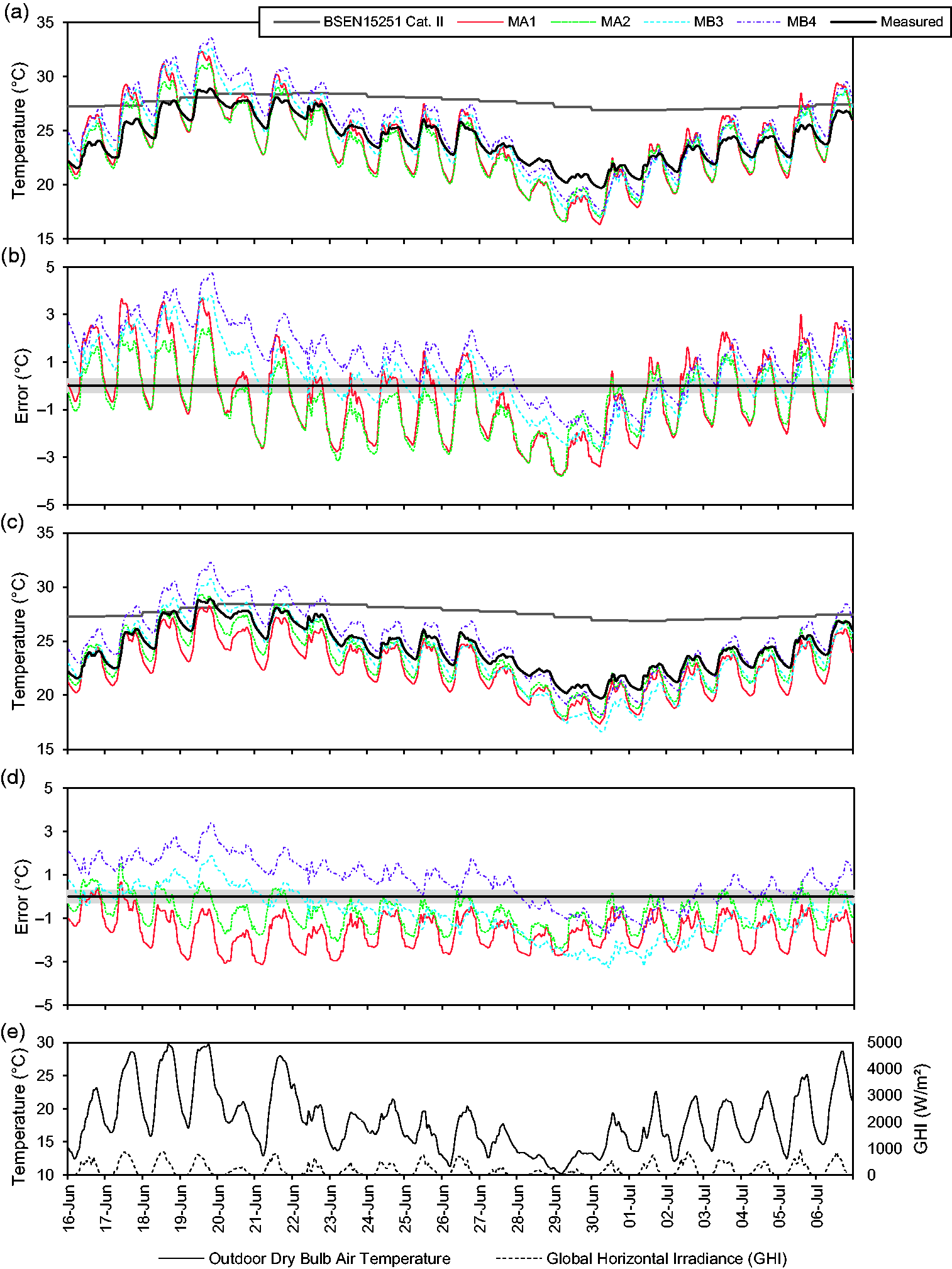
During the experimental period, both houses had the curtains open during the day, the East house had windows closed at all times (Experiment Eco), whereas in the West house, the windows were open if the room temperature exceeded 22℃ during occupied hours (Experiment Woo). Illustrative plots comparing the measured and predicted temperatures are shown for the living rooms and front double bedrooms only, Eco (Figures 3 and 4) and Woo (Figures 6 and 7) but the comparative statistics are provided for all the rooms in both houses (Tables 8 and 9) as are the measured and modelled predictions of hours of overheating (Figures 5 and 8). During the experiments, the highest measured operative temperature
y
in any room was recorded on 19 June in the single bedroom of the East house (32.2℃); the lowest was 19.2℃ in the kitchen of the West house on 30 June.
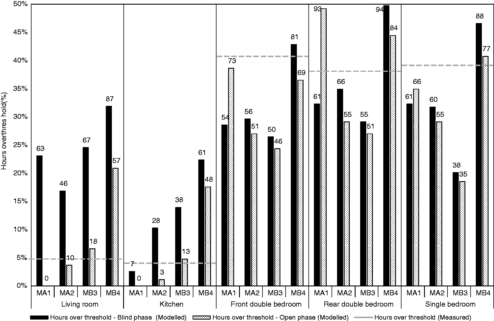
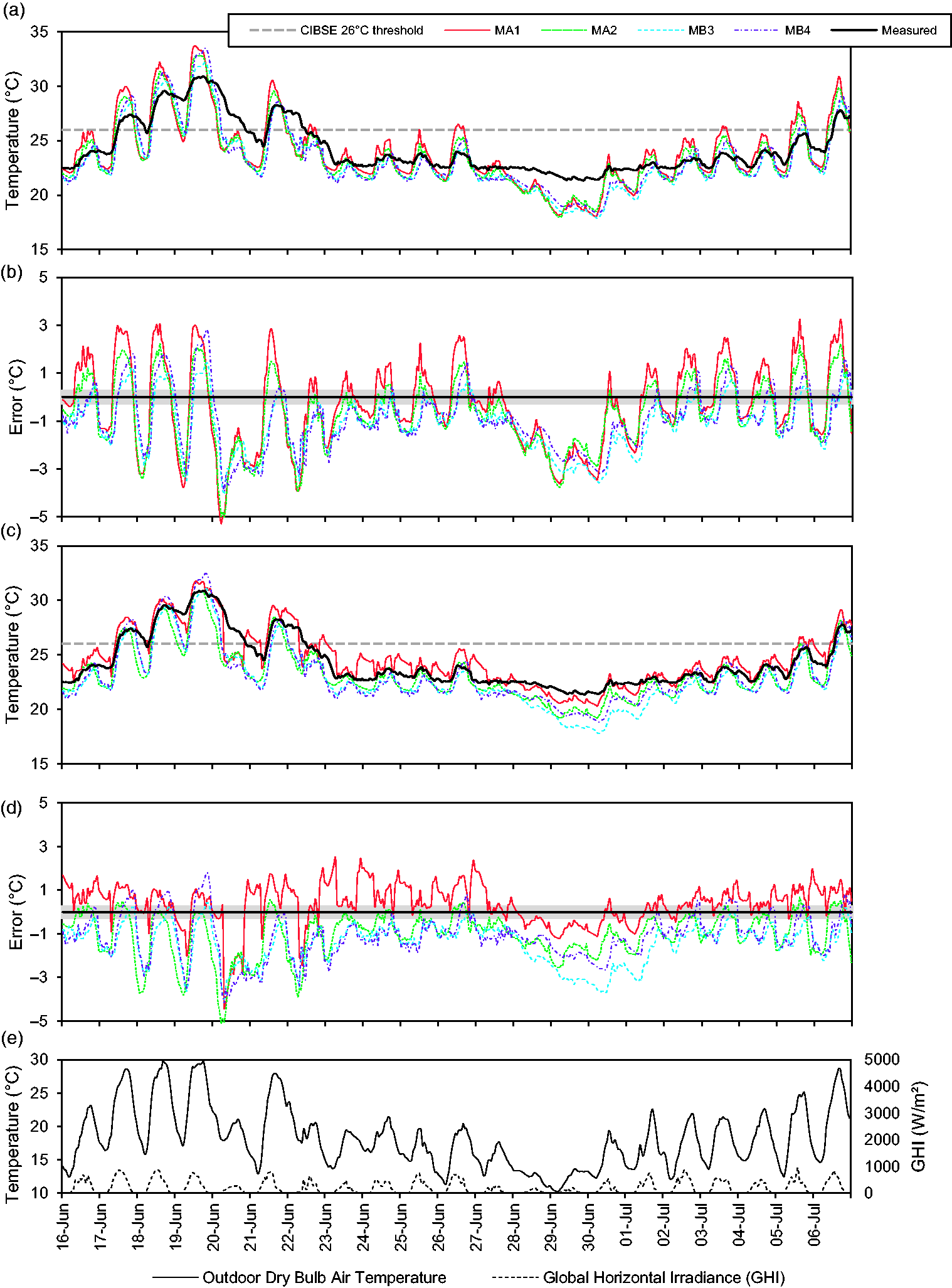
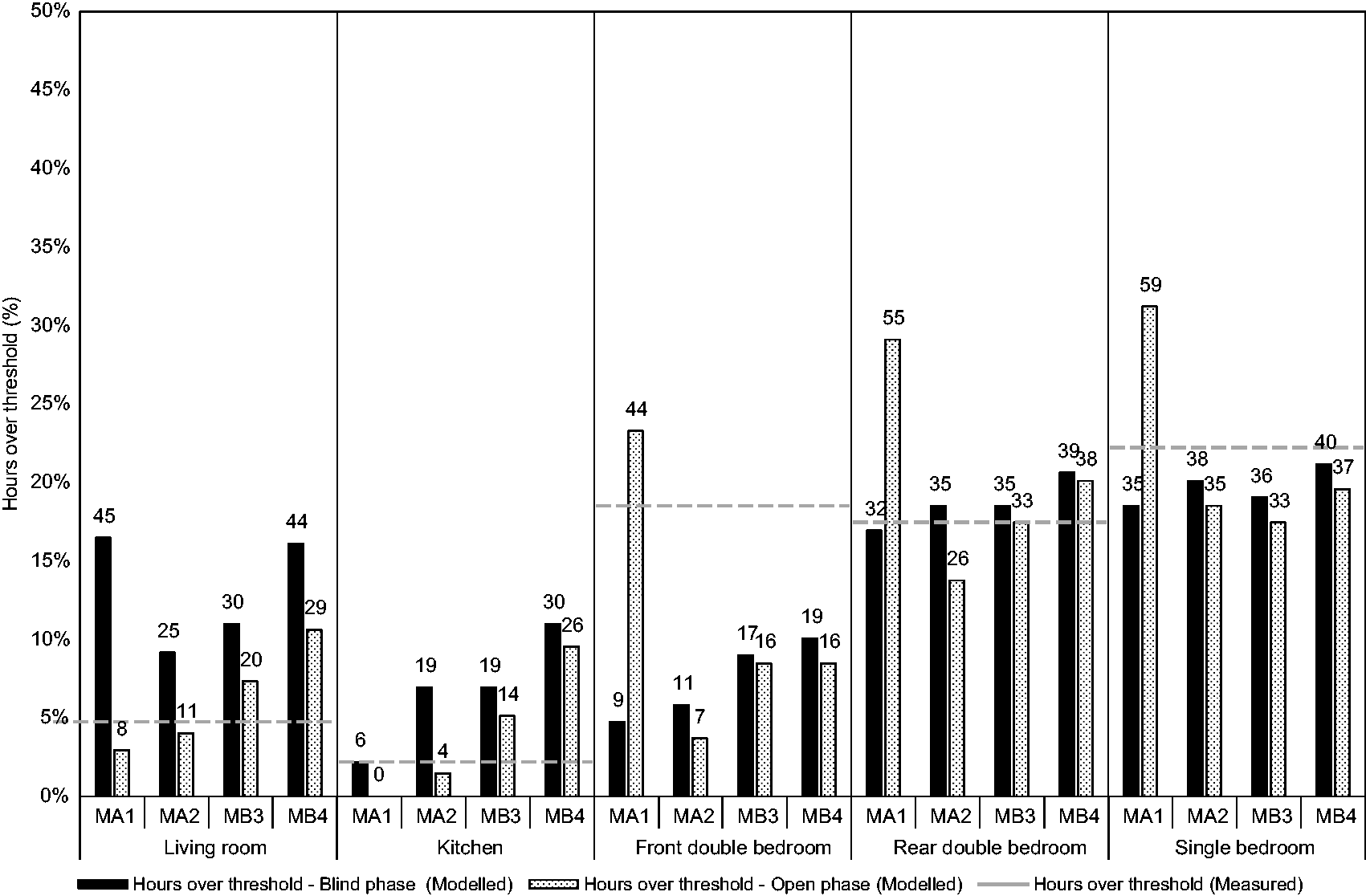
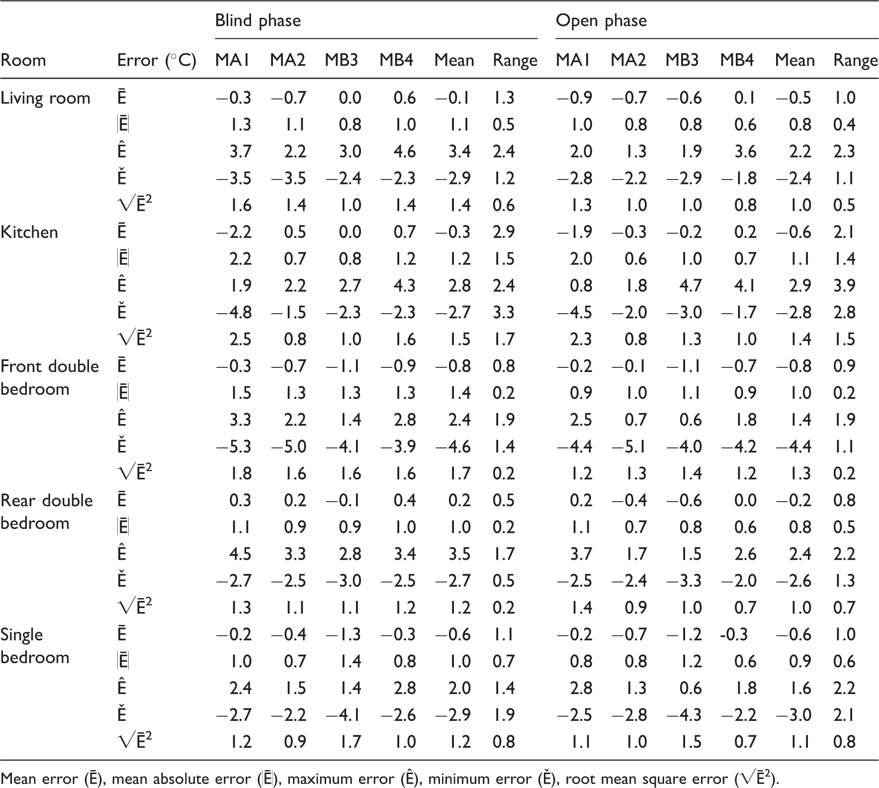
Experiment Eco: operative temperatures measured in the front bedroom and the temperatures predicted by each model: (a) measured and predicted, blind phase; (b) difference between measured and predicted, blind phase; (c) measured and predicted, open phase; (d) difference between measured and predicted, open phase; (e) outdoor air temperature and global horizontal irradiance. Grey shading around measurements on plots b and d indicate 0.3℃ measurement uncertainty. Experiment Eco: measured and predicted occupied hours of overheating: BSEN15251 Category II threshold in living room and kitchen and CIBSE threshold temperature of 26℃ for bedrooms. Numbers on bars are the number of hours above the overheating threshold. Experiment Woo: operative temperatures measured in the living room and the temperatures predicted by each model: (a) measured and predicted, blind phase; (b) difference between measured and predicted, blind phase; (c) measured and predicted, open phase; (d) difference between measured and predicted, open phase; (e) outdoor air temperature and global horizontal irradiance. Note: Grey shading around measurements on plots b and d indicate 0.3℃ measurement uncertainty. Experiment Woo: operative temperatures measured in the front bedroom and the temperatures predicted by each model: (a) measured and predicted, blind phase; (b) difference between measured and predicted, blind phase; (c) measured and predicted, open phase; (d) difference between measured and predicted, open phase; (e) outdoor air temperature and global horizontal irradiance. Note: Grey shading around measurements on plots b and d indicate 0.3℃ measurement uncertainty. Experiment Woo: measured and predicted occupied hours of overheating: BSEN15251 Category II threshold in living room and kitchen and CIBSE threshold temperature of 26℃ for bedrooms. Numbers on bars are the number of hours above the overheating threshold. Error statistics for experiment Eco: windows closed and curtains open during the day. Mean error (Ē), mean absolute error (|Ē|), maximum error (Ê), minimum error (Ě), root mean square error (√Ē2). Error statistics for experiment Woo: windows open in occupied rooms and windows operable to TM59 schedule, curtains open during the day. Mean error (Ē), mean absolute error (|Ē|), maximum error (Ê), minimum error (Ě), root mean square error (√Ē2).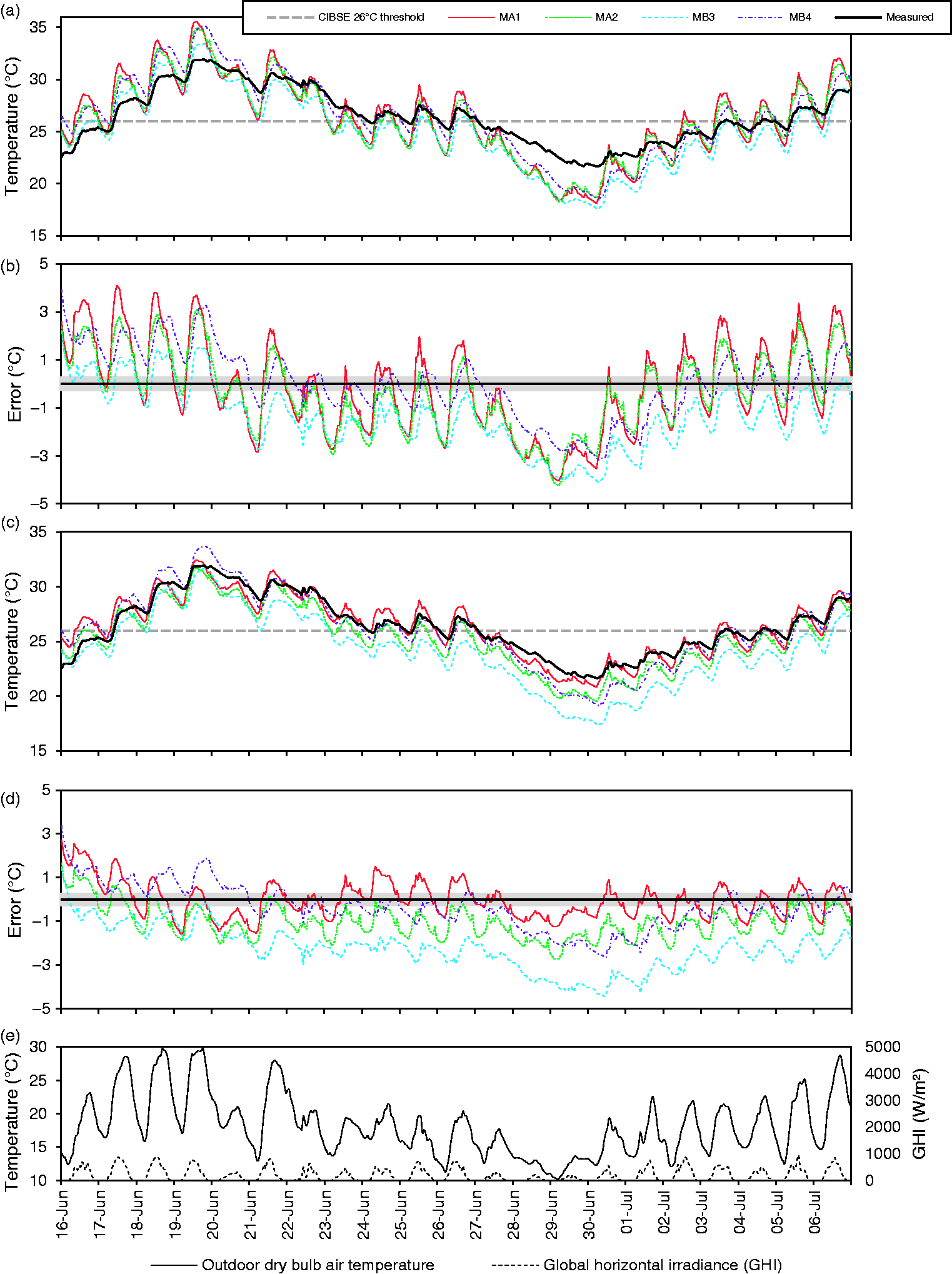
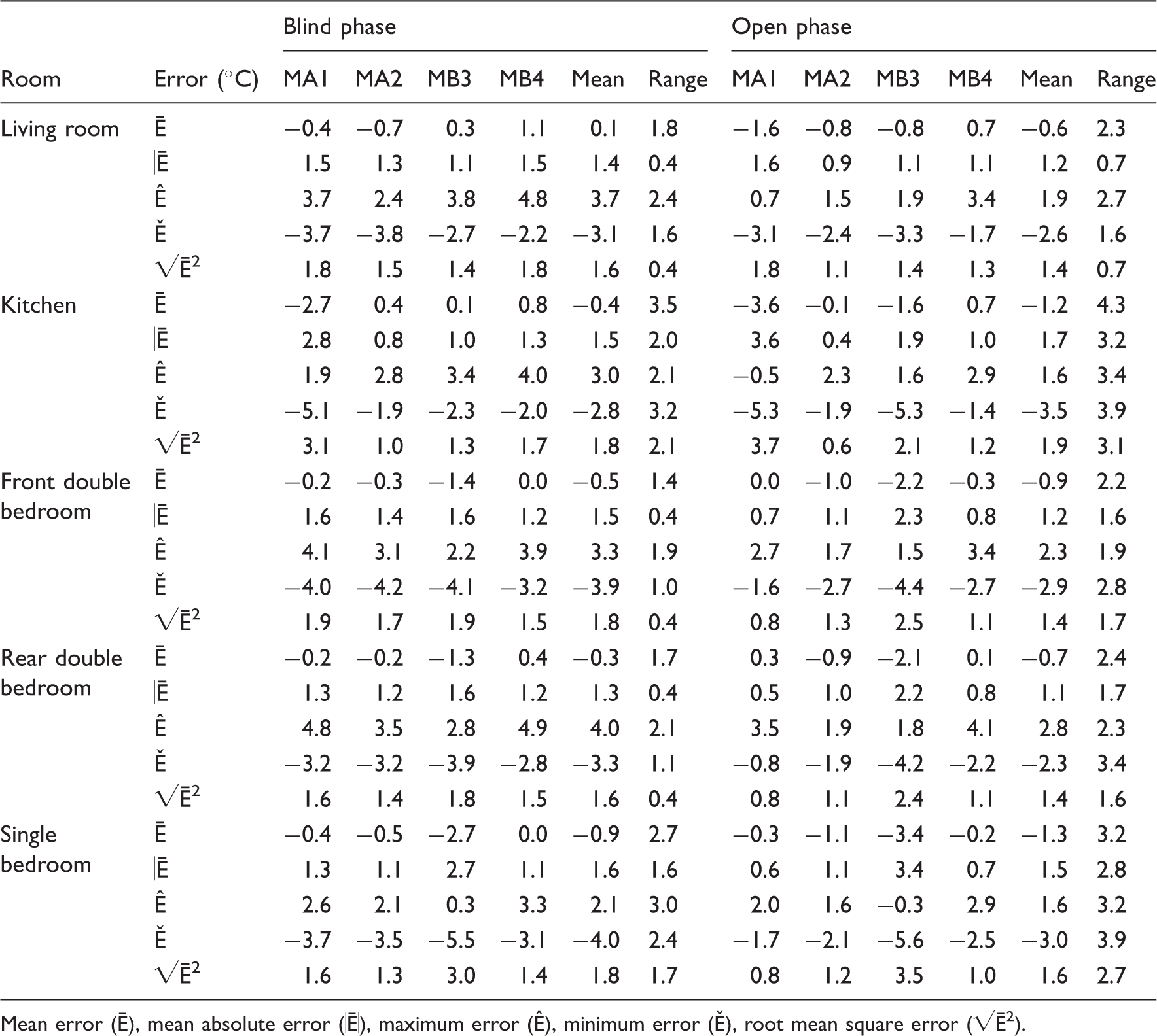
Experiment Eco: Windows closed and blinds and curtains open
Experiment Eco might be considered as unrealistic for an occupied urban house as the windows were kept closed at all times. The measured temperatures in the living room reached 28.9℃ on 19 June, the minimum was 19.7℃, in the early morning of 30 June (Figure 3(a) and (c)). The measured temperatures in the living room exceeded the BSEN15251 Cat. II threshold on the 18 and 19 June for 13 h (Figure 3(a) and (c)) which represented 5% of the occupied hours during the whole period (Figure 5). The temperatures measured in the bedrooms were higher than those recorded in the downstairs rooms. The peak temperature in the front double bedroom reached 31.9℃ (Figure 4(a) and (c)) with temperatures exceeding the 26℃ threshold during sleeping hours on 11 successive nights between 17 and 27 June and also between the 4 and 6 July. This resulted in overheating during 77 sleeping hours, i.e. 41% of sleeping hours during the experimental period (Figure 5). The measured sleeping hours of overheating were similar in all three bedrooms, even the north-facing rear double bedroom (Figure 5).
Turning now to the predicted temperatures for experiment Eco, during the blind phase the predicted living room temperatures had an overall RMS error (Table 8) of 1.4–1.8℃ depending on the model, z implying that temperatures were within ±2.7–±3.5℃ of the measured value for 95% of the experimental hours. However, the predictions were higher than those measured during the warm period (Figures 3(b) and 4(b)) with predicted peak temperatures exceeding the measured values by between 2.4 and 4.8℃ (Table 8). Thus, it was at just the time when predictions needed to be most reliable for assessing overheating that they displayed the greatest deviation from the measurements. The predictions also displayed much greater diurnal range than the measurements, e.g. between 5.2 and 7.5℃ on the 19 June compared to a measured range of 2.9℃. Thus, the predicted minimum temperatures in the living room were lower than those measured.
The higher predicted temperatures during the hot periods translated into substantially more predicted overheating hours in the living room (BSEN15251 Cat. II threshold) than was measured; predictions varying from 46 h, 17% of occupied hours (MA2), to 87 h, 32% of occupied hours (MB4); compared to 13 h, 5% of occupied hours as measured (Figure 5).
The predicted temperatures in the front bedroom during Experiment Eco also exceeded the measured values on the hot days (Figure 4(a) and (b)) by between 2.2 and 4.1℃ depending on the model (Table 8). As observed for the living room predictions, the predicted diurnal range in bedroom temperature was much greater than measured and the predicted minimum temperatures much lower than measured (Figure 4(a) and (b)). In the front double bedroom, the predicted sleeping hours of overheating (26℃ threshold) varied between the models from 50 h (26%) for MB3 to 81 h (43%) for MB4; with MA1, MA2 and MB3 predicting far fewer overheating hours than was measured (Figure 5). The predictions for the other bedrooms followed a similar pattern, with MB4 predicting slightly more overheating than measured and the other models somewhat fewer.
Overall, these results indicate that, although during the experiments, the overall mean error (i.e. difference between the predictions and the measurements) and the absolute mean error are small for all rooms (mean under 1.6℃) the models tended to over predict temperatures during the middle of the day, especially on hot sunny days and, because the diurnal range was also over predicted, tended to predict lower than measured night time temperatures. These same tendencies were manifest for all five rooms. These differences between the predicted and the measured temperatures translate into different outcomes with regard to overheating hours.
The modellers were struck by the differences between their predictions and the measured temperatures and how the differences occurred mostly on the sunnier days and at night. During the open phase, therefore, all four modellers made adjustments to their program's input data to try and improve the predictions (refer to ‘The open phase’ section). Consequently, for both the living room and front bedroom, the temperatures predicted on the warm days were lower than those predicted during the blind phase, and the diurnal temperature swings were less (Figures 3(c), (d), 4(c) and (d)), but still evident. The maximum temperature differences between the measured and predicted values were 0.7–3.4℃ (depending on the model) in the living room and 1.5–3.4℃ in the front bedroom (Table 8). Despite the changes to the models, the RMS errors were similar (Table 8), and there remained quite large differences between the predictions of peak temperatures.
The modellers discussed the possible reasons for these characteristic variations between model predictions. The modellers were frustrated that none of the parameters they varied closed the gap between measurement and prediction. Speculation turned to the underlying algorithms within the programs and particularly on how the models calculate the heat flux absorbed into and released by the building fabric. This perspective was supported by the observation that the relative ranking of the model predictions remained substantially the same in both the blind and open phases. For example, in all three bedrooms, MB3 predicted the lowest overheating hours, MA2 the next lowest and MB4 the most overheating hours (Figure 5, Table 8). The way the programs are used also has an influence (program A users predicted both the highest and lowest overheating hours, respectively).
It is also worth noting that the relative ranking of models' predictions varies from room to room. For example, in the open phase, MA1 predicted the lowest overheating hours in the downstairs rooms, but in the bedrooms, MA1 predicted the second highest overheating hours (Figure 5). Thus, it would be difficult to identify one modeller or program as tending to consistently over predict overheating risk and another tending to consistently under predict the risk.
Experiment Woo: Windows operable
In experiment Woo, the windows were open during occupied hours if the room temperature exceeded 22℃, which is the specified CIBSE TM59 window opening profile. The peak measured temperatures in all the rooms were generally lower than when the windows were always closed (Experiment Eco) (Figures 6 and 7, cf. Figures 3 and 4). The living room reached 28.5℃ on 19 June, and the minimum temperature was 19.4℃ in the early morning of 30 June (Figure 6(a) and (c)). The measured living room temperatures exceeded the BSEN15251 Cat. II overheating threshold for 13 occupied hours (Figure 8), which is the same as when the windows were closed (Experiment Eco) (Figure 5).
As in Experiment Eco, the bedrooms were warmer than the downstairs rooms with a peak temperature in the front bedroom of 30.9℃ (Figure 7(a) and (c)). Temperatures over 26℃ occurred during sleeping hours between 17 and 22 June for 35 h, i.e. 19% of sleeping hours during the whole period (Figure 8). The overall effect of the window operation was therefore to substantially reduce the measured hours of bedroom overheating, by about 22 percentage points (pp) in the front double bedroom, i.e. from 41% (Eco) to 19% (Woo), and by between 17 and 21 pp in the other two bedrooms (Figure 9).
Measured and predicted differences in overheating hours as a result of opening windows over: BSEN15251 Category II threshold in living room and kitchen and CIBSE threshold temperature of 26℃ for bedrooms. Numbers on bars are the difference in the number of hours above the overheating threshold.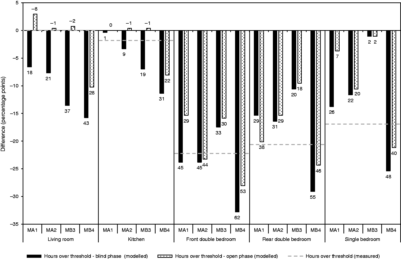
Turning to the predicted temperatures, it is apparent that in the blind phase the peak temperatures exceeded the measured temperatures on warm days, by 2.2–4.6℃ in the living room (Table 9), which is similar to the result when the windows were closed. In the front bedroom, however, predicted peak temperatures exceeded the measured values by 1.4–3.3℃ (Table 9), which is better than in experiment Eco. However, there was a greater diurnal swing compared to the measured swing than was observed in experiment Eco, suggesting that the models were over predicting the impact of the window opening. This was most marked in the front bedroom (Figure 7(b)) but also evident in the living room (Figure 6(b)). It is possible that the blinds impeded air flow at night in the test houses although they were assumed not to in the models.
The overall effect was that the models tended to over predict the number of overheating hours in the downstairs rooms, under predict for the front double bedroom and produce predictions that were similar to, and straddled, the measured overheating hours in the other bedrooms (Figure 8). The variability in the predicted hours of overheating between the models was also much less than in Experiment Eco, e.g. between 25 (MB2) and 45 h (MB1) in the living room and between 17 (MB3) and 19 h (MB4) in the front double bedroom (Figure 8).
In the open phase, following the refinement of the model input data, the diurnal swings in temperature in the downstairs rooms were reduced but were still much larger than was measured (cf. Figure 6(d) and (b)). In the bedrooms, however, predicted decrease in the night time hourly temperatures compared to the measurements was still evident, with a much sharper drop in the predicted temperature when the windows opened than was measured (cf. Figure 7(d) and (b)).
The changes to the predicted hours of overheating as a result of model refinement in the open phase were less marked than for Experiment Eco, with only small changes in predictions for models MA2, MB3 and MB4. Thus, the patterns of over and under-prediction that were observed in the blind phase prevailed in the open phase.
Effect of window opening
In a design context, it is important to know if models correctly predict the impact on overheating of a change to a dwelling and how accurately the magnitude of the change is predicted. Encouragingly, with five small exceptions, all the models correctly predicted that opening the windows would reduce the incidence of overheating and all but MB3 that the greatest reduction would occur in the bedrooms – as indicated by the measurements (Figure 9). The predicted changes in overheating were similar for the blind and open phases in the bedrooms, but showed greater variation in living rooms.
Inter-model comparison using DSY weather data
In addition to making predictions of the temperatures in the experimental houses, the modellers also made predictions of the annual incidence of overheating using the procedure and Criteria recommended in TM59. 12 It is therefore possible to compare the extent of agreement, or otherwise, in the models' identification of rooms that are deemed to be overheated. The Simulation Resolution, which is a measure of inter-model variability, could then be estimated.
Each modeller used the house descriptions they created in the blind and open phases and the DSY1 weather file for Nottingham (2020s, high emissions, 50th percentile scenario). Three comparisons (C) were made, each with a different window opening and shading schedule (Table 3).
Cco: with windows closed and the shading open (as in Experiment Eco), Coo: with the windows opening according to the TM59 protocol and the shading open (as in Experiment Woo), Coc: with the windows opening and the shading closed.
aa
Prediction of annual overheating risk in each house using TM59 Criteria and DSY1 weather year for Nottingham (bold indicates failing the Criteria). Criterion A: Values are a percentage of the occupied hours between May and September, which were: living room and kitchen 1989 h; bedrooms 3672 h. Criterion A is failed if the percentage value exceeds 3%. Criterion B: Values are a percentage of annual occupied hours between 22:00 and 07:00 in the bedrooms: 3285 h. Criterion B is failed if the percentage value exceeds 1%.
For each comparison, the percentage of hours exceeding the Criterion A thresholds (all rooms) and the Criterion B threshold of 26℃ (bedrooms only), and whether the result represented a pass or fail, was determined (Table 10). To pass, overall bedrooms must satisfy both criteria.
12
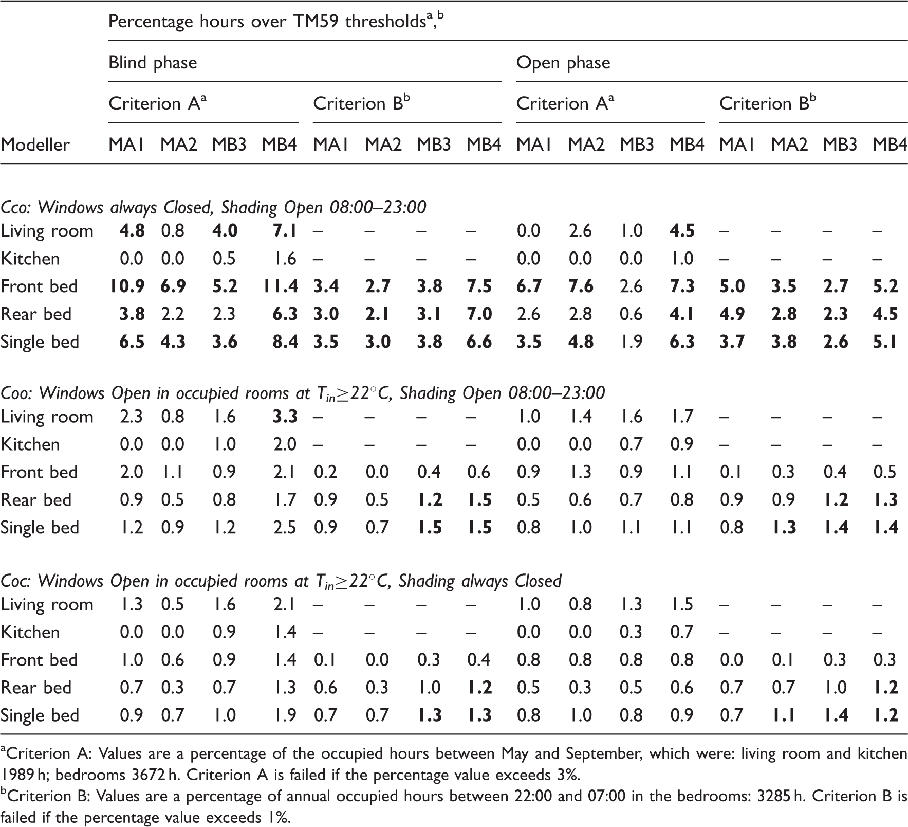
With the windows closed (Cco), all four models predicted that bedrooms would clearly fail Criterion B, the smallest number of predicted hours over the 26℃ threshold in any room was 2.1% (Table 10), more than twice as many hours as the 1% allowed by TM59 (Figure 10(b)).
Inter-model comparison Cco: predicted annual occupied hours over: (a) TM59 Criterion A threshold and (b) TM59 Criterion B threshold. Numbers on bars are the number of hours above the overheating threshold.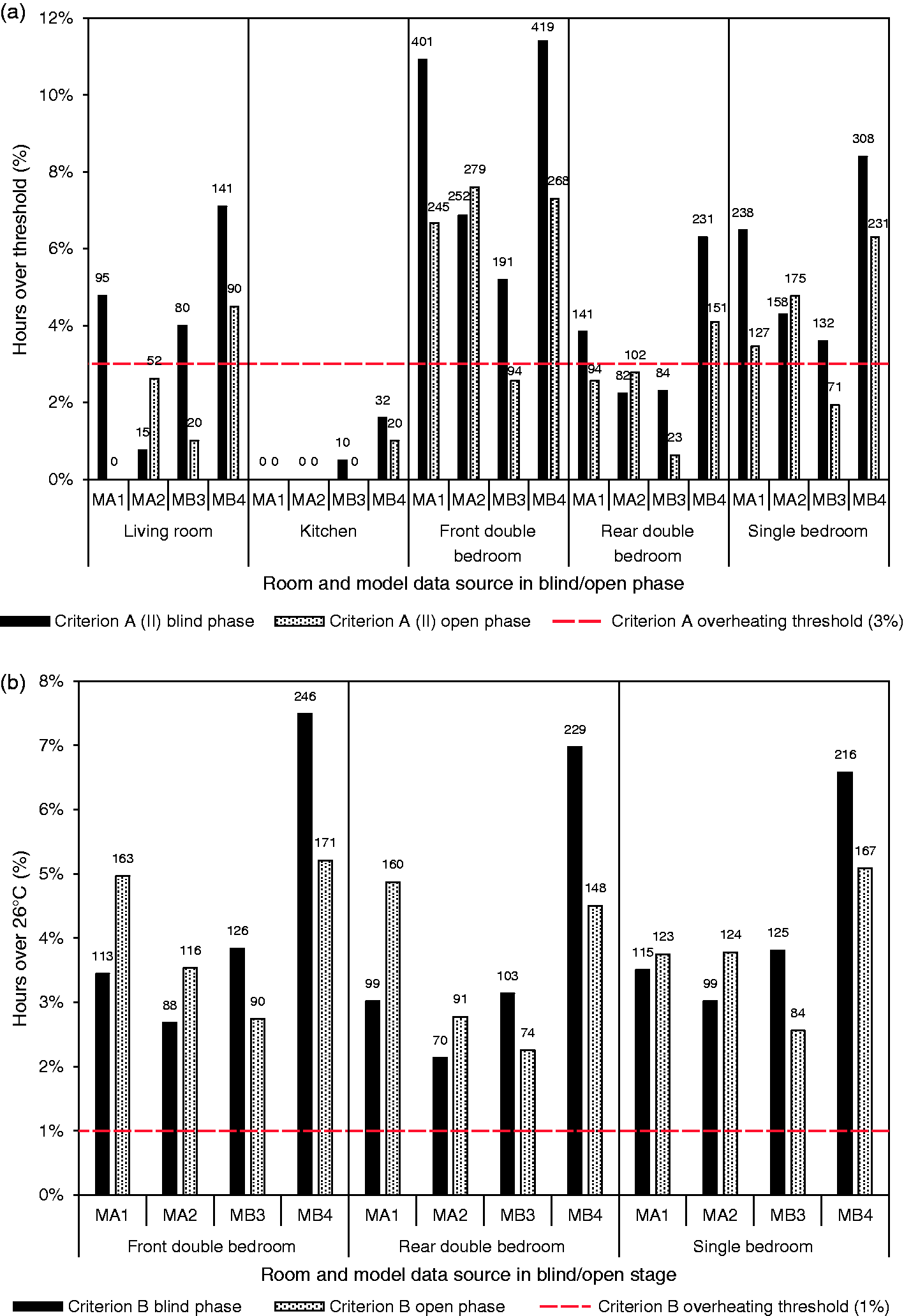
For both the blind and open phase models, some models predicted that some bedrooms would fail Criterion A but others that they would not. Using the open phase models, MB3 predicted that all bedrooms would pass yet MB4, using the same DTS program, that all would fail. Using their open phase models, all modellers predicted that the north-facing kitchen would not overheat but there was divergence between the assessment of the living room, between MB4 and the other models.
For inter-model comparisons Coo and Coc, for which the windows were operated in accordance with TM59,
bb
the overall pass/fail agreement between the models was much improved (Table 10, Figure 11).
Inter-model comparison Coo: predicted annual occupied hours over: (a) TM59 Criterion A threshold and (b) TM59 Criterion B threshold. Numbers on bars are the number of hours above the overheating threshold.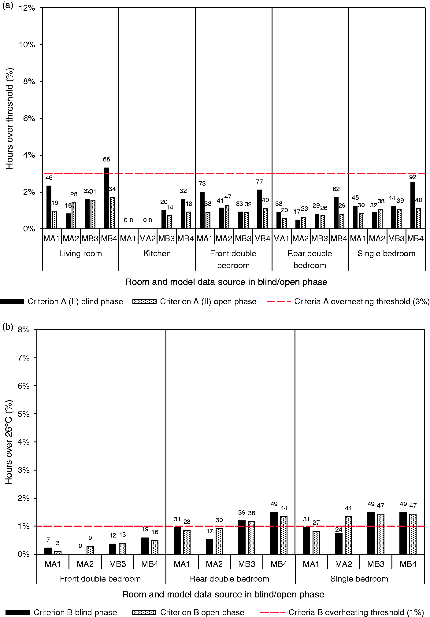
Using Criterion A, all four modellers, with both their blind or open phase models (with one minor exception), clearly predicted that none of the rooms would overheat (Figure 11, Table 10). For Criterion B, the predicted overheating percentages hovered close to the pass/fail boundary. All the models predicted that the front bedroom would overheat less than the rear and single bedroom by Criterion B; however, the users of model B predicted that the rear and single bedroom would fail Criterion B whereas the users of model A predicted that they might not.
When predictions are close to Criteria pass/fail boundaries, any variability in models’ predictions can result in a different pass/fail outcome. Therefore, knowing the resolution of predictions can assist modellers in deciding whether or not their overheating assessments are sufficiently robust to determine clearly whether a room passes or fails one or other Criteria, this matter is addressed in the ‘Simulation Resolution’ section.
In a design context, it is often important to know whether the difference in overheating as a result of a design change is reliably predicted. Comparing the results of inter-model comparison Coo with Cco (Figure 12), it is clear that the models were consistent in their prediction that overheating in the bedroom would decrease, as measured by either Criterion. There was, however, considerable variability in the predicted decrease in overheating hours. For example, for Criterion A, in the front double bedroom (open phase models), a decrease of 62 h was predicted by model MB3 compared to a decrease of 232 h predicted by model MA2. For the downstairs rooms, using Criterion A, the models predicted a much smaller reduction in overheating hours as a result of the window opening, and, with open phase models, MA1 and MB3 determined that window opening would actually increase the hours of overheating (other two models predicted the opposite effect). Knowing how reliable models are for predicting differences between competing design options would also be a useful aid to modellers.
Predicted difference in annual overheating hours as a result of opening windows: (a) over TM59 Criterion A threshold and (b) over TM59 Criterion B threshold. Numbers on bars are the difference in the number of hours above the overheating threshold.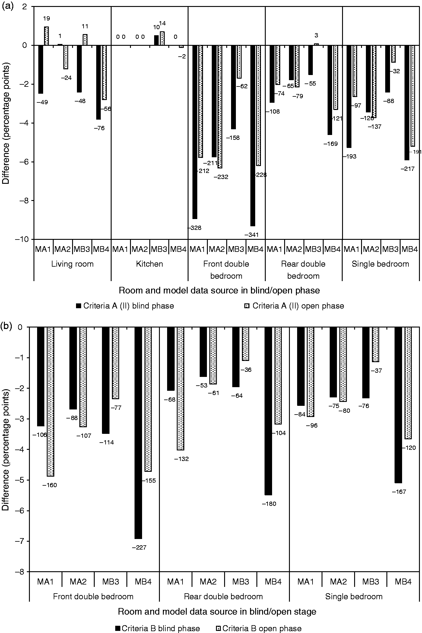
Simulation Resolution
Simulation Resolution seeks to answer the question ‘if a different, reputable DTS program were used by a skilled person for the same overheating analysis, by how much might the predictions vary?’. It is a value that could vary depending on the dwelling and room being analysed, the annual weather file used for the predictions and the overheating Criterion. By knowing the SR of dynamic thermal model predictions, it would be possible for modellers to know whether or not they could confidently assert whether a room (or dwelling) has passed or failed an overheating Criterion. A tentative formal definition of SR has previously been proposed
22
as: The Simulation Resolution, SR, is the value below which the absolute difference between the predictions of two programs (obtained by skilled users, for the same circumstances) may be expected to lie with a specified probability. In the absence of any other indication, the probability is 95%. Mean, minimum, maximum and range of predictions of annual overheating risk in each house using TM59 Criteria and DSY1 weather year for Nottingham. Criterion A: Values are a percentage of the occupied hours between May and September, which were: living room and kitchen 1989 h ; bedrooms 3672 h. Criterion B: Values are a percentage of annual occupied hours between 22:00 and 07:00 in the bedrooms: 3285 h.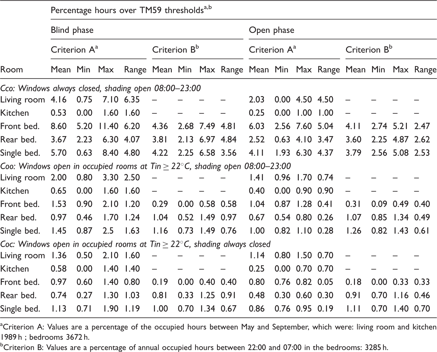
Although the number of results is small, a sense of the likely magnitude of the SR can be obtained by pooling the results for all three inter-model comparisons. The range in models' predictions as the mean predicted overheating hours increases is illustrated in Figure 13. For Criterion A, the range at a mean prediction of 3% overheating hours is same for both the open of blind phase models and is approximately 3 pp: this is the proposed SR value. Thus, if a DTS program predicts a Criterion A result that is 3% ± 3 pp, it would not be possible to assert with confidence whether the room/dwelling passes or fails the Criterion. For Criterion B, the SR values at 1% of overheating hours are estimated as 0.5 pp for the open phase models and 1 pp for the blind phase models; the latter most closely resembling the situation encountered in design practice. Thus, if a DTS program predicts a Criterion B result that is 1% ± 1 pp, determination of whether the room/dwelling passes or fails the Criterion would be unreliable. That the SR values are of a similar magnitude as the actual Criterion values might seem disappointing but, as noted earlier, the prediction of overheating is a particularly difficult task for DTS programs.
Comparison of range in model predictions with the mean predicted annual hours over: (a) TM59 Criterion A threshold and (b) TM59 Criterion B threshold.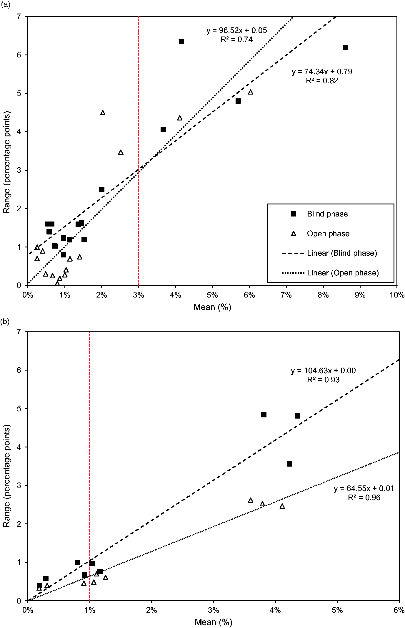
This analysis is intended to demonstrate the value of the SR concept, but many more inter-model comparisons are needed, both to fully test the SR concept, and to determine appropriate SR values for predictions at the Criteria pass/fail boundaries for different dwelling archetypes, overheating mitigation measures and weather conditions.
Discussion
Reflecting on the results of this study, it is worth considering their implications given the ways in which DTS programs are used in practice. Essentially, three types of prediction might be required: first, to determine if one design option is more or less likely to lead to overheating than another. Such predictions are used to drive the design of a new building or overheating mitigation retrofit towards a superior solution. Second, to predict by how much one option overheats compared to another, i.e. correct prediction of the difference in overheating hours between two or more competing options. This allows the efficacy and (cost) effectiveness of alternative design and retrofit options to be compared. Third, to predict the actual hours of overheating using a defined methodology when provided with the same weather data and occupancy profiles etc. cc as experienced by the actual building. The expectation placed on the accuracy of predictions becomes progressively more onerous from the first to the last of these types of prediction. The reliability of all three types of prediction depends on the inherent accuracy of the program and the way it is used (input data, choice of alternative modelling algorithms, etc.). The combination of inter-model comparison and empirical validation, using measured temperature data in houses with synthetic occupancy, has enabled the reliability of the user and DTS programs for all three types of prediction to be evaluated.
Robust prediction requires the reliable representation of the thermo-physical processes acting on an individual zone, such as a bedroom or living room. Most obvious of these are the weather conditions and the internal heat gains, but assumptions about the temperatures in adjacent zones and the connection to the modelled zone, by conduction and advection, are also important. The experiments undertaken for this research and the properties of the dwellings that influence these heat flows were well defined, potentially much more tightly than when tackling ‘real world’ design problems, especially those concerned with existing occupied buildings, to be retrofitted in order to curb overheating. Nevertheless, there is uncertainly in many of the data inputs required by DTS programs. In previous empirical validation studies, Monte-Carlo analysis has been used to quantify the effect of these data uncertainties on model predictions. Such an analysis was beyond the scope of this project.
Overheating prediction requires accurate representation of the individual zones in a building, especially the zones most at risk of overheating. This is fundamentally different to the DTS models built for annual energy demand prediction which might consist of dozens of zones. In such models, the under-prediction of energy demand in one zone might trade off against the over-prediction of energy demand in another, thus leading to a reasonable overall energy demand value. Furthermore, annual energy use is essentially the integral (area under) a power/time curve which might extend over the 8760 h in a year.
Overheating prediction is quite different and far more onerous than energy demand prediction, requiring accurate temperature prediction for a handful of hours only, e.g. for TM59 Criterion B around 33 h in the whole year. Over-prediction of temperatures at 1 h cannot be traded off against under-prediction of temperatures at another hour. Further, it is the hours in the year when the heat fluxes are greatest and are varying most rapidly for which accurate predictions are needed. (Solar radiation heat gains, the coupling between the air-point of the zone and the surrounding thermal mass and the advection between zones are all difficult processes to represent in DTS models).
To make reliable overheating predictions in a real design context, modellers have to focus down on the way the thermodynamic processes acting in individual zones are represented, especially the zones most at risk of overheating. These might include the fine details of site shading (trees, adjacent building, orientation), self-shading (overhangs, glazing bars, etc.), window transmission, ventilation opening types, sizes and blockage, e.g. by curtains, inter-zonal air flow and the actual thermal mass in each space. For overheating prediction, such details might really matter; dd for annual energy demand prediction, they might matter much less. Therefore, it might well be that the approximations that modellers (necessarily) make when modelling the annual energy demand of whole buildings, for example to assess compliance with carbon emission requirements, are wholly inappropriate when trying to accurately predict the risk of overheating. It may well be that further guidance about the design details that matter for overheating risk assessment, and how these should be represented in models could improve the repeatability and accuracy of overheating risk prediction.
Because of the sensitivity of predictions to chosen model inputs, there is perhaps the need for much more guidance about how to model buildings when overheating is being predicted. Guidance is required over many features of a building, with clarity given over which features need to be modelled precisely and which less so. For example, the assumptions made about the ‘active’ thermal mass in spaces and the window ventilation rates and how these change if curtains are drawn. What are the appropriate rates for other ventilation devices, such a window side panels, or deeply recessed opening? In overheating prediction, such details matter. Clear, precise guidance will narrow the differences in the predictions of different modellers.
Although the modellers tried to close the gap between predictions and measurements in the open phase of the work, differences remained. The differences suggested, as have previous researchers, that the way thermo-physical processes are represented in the programs need to be scrutinised. In particular, the operation of algorithms that determine the transfer of heat into and out of thermal mass, which influences the peak and diurnal swing of room temperature. Previous researchers have pointed out the sensitivity of temperature predictions to internal HTC algorithms.22,23
In this paper, it has been suggested that when predictions are within about 1 pp of the TM59 Criterion B limit of 1% of overheating hours (annual hours 22:00–07:00) or within about 3 pp of the Criterion A limit of 3% (occupied hours between May and September), then it is not possible to reliably assert whether the Criteria are passed or failed. In essence, the measuring tool that we have, a DTS program, is not accurate enough to resolve more finely than this. The SR figures are indicative, and more inter-model comparisons are needed to determine the SR values appropriate for different buildings and weather locations. Other ways of accommodating the uncertainty in DTS predictions might be possible, but it is important that it is accounted for somehow, especially if overheating risk assessment becomes a regulatory requirement.
Validation of dynamic thermal models is an essential step in the drive towards more accurate prediction and thus more robust building design. However, validation is not a one-off enterprise and a model's reliability for making one type of prediction will differ from its reliability when making another type of prediction. The data provided to modellers in this paper is made openly available to enable the validity of overheating predictions for conventional UK homes to be quantified.45
Conclusion
There is a concern about the incidence of summertime overheating in UK homes, and so regulation is being considered to curb the building of new homes that are at risk of overheating. DTS programs are widely used to predict the risk of summertime overheating. Previous research work has shown, however, that the prediction of overheating is an inherently difficult problem for DTS programs to resolve. Different programs, even when provided with near-identical input data, can produce very different predictions of overheating risk. Differences in the way programs are used can exacerbate inter-model variability. The recent CIBSE Technical Memorandum, TM59, provides guidance which seeks to reduce inter-model variability.
This paper reports comparisons between the summertime temperatures measured in five rooms in two test houses and the predictions of two different DTS programs used by four different modellers, i.e. empirical validation. The inter-model variability in the four sets of predictions, when used to predict the annual overheating risk of the houses using the TM59 protocol, is also quantified, i.e. an inter-model comparison. For both types of prediction, modellers first made blind predictions, i.e. with information about the houses and the weather conditions but without knowledge of the measured temperatures or the approaches being used by other modellers. In the subsequent open phase, modellers made new predictions having had access to the measured temperatures and the opportunity to discuss their modelling strategy with the other modellers.
The measurements were made in two adjacent, near-identical, 1930s, semi-detached houses, over the same 21-day period, which included a spell of hot weather. Both houses had synthetic occupancy, which mimicked that specified in TM59. In one house, the windows were closed at all times and in the other open when the room air temperatures exceeded 22℃, which is perhaps more realistic of real occupant behaviour and is as specified for TM59 analyses. In the house with closed windows, the peak temperatures in the living room reached 28.9℃ and in the front double bedroom 31.9℃. With operable windows, the peak temperatures were 28.5℃ in the living room and 30.9℃ in the front double bedroom.
In the blind phase, in both houses, the greatest deviation from the measurements occurred on the warm days, i.e. on precisely the days when predictive accuracy is most needed. On such days, all four models over predicted the peak indoor temperatures. For example, on the warmest day, in the house with operable windows, the predicted peak temperatures exceeded the measurement by between 1.4 and 3.3℃ in the front double bedroom and between 2.2 and 4.6℃ in the living room. In both houses, the models therefore predicted more occupied hours in the living room over the BSEN15251 Cat. II threshold than was measured.
The models also tended to over predict the diurnal swing in indoor temperature. Consequently, in the house with windows closed, all the models predicted fewer sleeping hours in the bedroom over 26℃ hours than measured. For the house with the windows open, the modelled and measured sleeping hours in the bedrooms over 26℃ were similar for two of the bedrooms.
In the open phase, all four modellers were able to improve the prediction of hourly room temperatures during warm weather, suppressing, but not eliminating, the over-prediction of peak temperatures and diurnal swing. The prediction of overheating hours in the living rooms improved, but in the bedrooms, the differences between modelled and measured overheating hours remained largely unchanged.
Differences between measurement and predictions were partly due to the way the models were used. However, the tendency of the models to over predict peak temperatures, which could not be suppressed when the modellers made reasonable modifications to program inputs, suggests that the DTS programs themselves contribute to the differences. In particular, the way that internal algorithms handle the thermo-physical processes that determine indoor temperature on hot (sunny) days.
In addition to making predictions of the temperatures in the experimental houses, the modellers also made predictions of the incidence of overheating using the DSY1 (2020s, high emissions 50th percentile scenario) for the local region following the procedures and Criteria recommended in TM59. For houses with operable windows, as specified by TM59, all four models, in both the blind and open phase (with one minor exception), predicted that none of the five rooms would overheat during occupied hours (Criterion A). For the bedrooms, the predicted percentage of sleeping hours hovered close to the Criterion B pass/fail boundary.
To quantify the uncertainty in models' TM59 predictions, the concept of Simulation Resolution (SR) was invoked. The SR indicates by how much the predicted hours over the threshold might change if a different DTS model was used to undertake the same analysis. For TM59 Criterion A, the estimated SR at the pass/fail boundary was 3% ± 3 pp and for TM59 Criterion B, 1% ± 1 pp in the blind phase. Thus, when predictions are within about 1 pp of the TM59 Criterion B limit of 1% or within about 3 pp of the Criterion A limit of 3%, then assessment of whether the Criteria are passed or failed is unreliable.
Further research is also required to understand the causes of variation between model predictions of overheating and the reason for the differences from the measured temperatures. It is argued that more detailed guidance on how to model the features of buildings that have a material impact on overheating assessments could help reduce the variability between the results of different modellers.
Nevertheless, there will always be variability between the predictions of different DTS programs, and so work should be done to test the utility of the SR concept in the real design context, to refine the approach to determining SR values and to calculate the SR for a range of dwelling archetypes, overheating mitigation measures and weather conditions.
Footnotes
Acknowledgements
The authors wish to thank the four modellers who gave their time to this research. We acknowledge CIBSE for their provision of DSY1 weather data. We thank Mr Jim Muddimer (Loughborough University) who maintained the School of Architecture, Building and Civil Engineering weather station. We also thank Dr Richard Hodgkins and Dr Tom Betts (both Loughborough University) for supplying weather data from the School of Geography and Environment weather station, and the School of Mechanical, Electrical and Manufacturing Engineering weather station, respectively. We acknowledge Loughborough University's continued provision of 24-h security and the ongoing maintenance of the test houses. The authors are also grateful to the reviewers, whose comments led to improvements to this paper, identifying the value of detailed guidance for modellers engaged in overheating risk prediction and affirmation that Simulation Resolution is useful in interpreting such predictions.
Declaration of conflicting interests
The author(s) declared no potential conflicts of interest with respect to the research, authorship, and/or publication of this article.
Funding
The author(s) disclosed receipt of the following financial support for the research, authorship, and/or publication of this article: London-Loughborough Centre for Doctoral Research in Energy Demand (grant EP/L01517X/1).