
Abstract
Fluid catalytic cracking (FCC) is an important process in petroleum processing. Effective monitoring of the status and quality of FCC is vital. Accurate description of the relationship between process and quality variables is the basis of quality-driven monitoring. Many process variables affect the quality of FCC; some of these effects are linear, and others are nonlinear. We propose a combination method from the perspective of linearity and nonlinearity to improve the monitoring performance of FCC quality. Partial least squares (PLS) is initially used to extract linear features, and its residual space is saved as the input of the deep feedforward neural network (DFNN). DFNN is then used to extract nonlinear features for the further decomposition of subspaces. The PLS-DFNN method accurately describes processes involving linearity and nonlinearity. We construct three monitoring statistics to characterize the types of faults. The proposed method proves its excellent effect on a numerical simulation data set. It effectively distinguishes the types of faults on the Tennessee Eastman process data set, and the fault detection rate is superior to other related methods. Finally, we apply this method to the actual FCC and verify the superiority of this combination.
Keywords
Introduction
Fluid catalytic cracking (FCC) is a vital process to lighten heavy oil in petroleum processing (Ancheyta et al., 2004; Vistisen and Zeuthen, 2008). FCC, as the main process to produce transportation fuel and provide part of low carbon olefin, has outstanding advantages and irreplaceable role. FCC has the advantages of strong feedstock adaptability, high yield of light oil products, and mature technology; it is therefore an important source of profit for oil refining enterprises at present (Han and Chung, 2001; Lz and Hdl, 2019). The deterioration of heavy crude oil, the rising market demand for light oil products, and the increasing pressure on clean fuel production and environment in recent years have accelerated the process of refining integration. Global refineries speed up the adjustment of process equipment structure, while the core position of FCC, as the main process conversion unit, remains unchanged (Li et al., 2020; Lin and Zeng, 2013). However, the process of FCC, which includes reaction regeneration, fractionation, absorption and stabilization, and desulfurization and denitrification systems, is complicated; each system also involves multiple towers (Lopez-Zamora and de Lasa, 2019). System performance is not only closely related to economic benefits but also may lead to potential safety hazards (Jiang et al., 2020b). Process monitoring has been highly valued for ensuring the long-term reliable operation of such complicated processes. Classical monitoring methods based on models or prior knowledge have failed to work well; thus, data-driven methods are bound to develop rapidly because of the wide use of new measurement technologies and the considerable progress in data mining (Bounoua et al., 2019; Ge, 2017; Jiang et al., 2019; Li and Feng, 2020; Theisen et al., 2021; Yao et al., 2022). Multivariate statistical process monitoring (MSPM) methods are fairly representative of data-driven methods. They extract low-dimensional features from high-dimensional data, and then, they establish monitoring statistics in low-dimensional spaces (Bounoua et al., 2019; Ge, 2017; Jiang et al., 2019). The two main methods are principal component analysis (PCA) (Kano et al., 2001) and partial least squares (PLS) (Qin and Zhou, 2010). The former performs orthogonal projection on the feature space, while the latter performs oblique projection on the feature space.
Quality-driven methods have elicited increasing attention in recent years. The process can be better controlled by monitoring whether quality has been influenced (Huang and Yan, 2019; Yan et al., 2019). However, obtaining quality variables is costly and time consuming; we cannot guarantee the real-time acquisition of quality variables in online monitoring. Thus, the quality information contained in process variables should be found in offline modeling. PLS is commonly used to establish the relationship between process variables and quality variables. PLS extracts components that reflect the regression relationship between process variables
However, the FCC process consists of multiple units and a large number of process variables. The effects of these variables on the product quality are uncertain; some of these effects are linear, and others are complex nonlinear. The above linear methods may not be applicable to complex nonlinear processes. Therefore, kernel tricks are introduced. Peng et al. (2013) first proposed total kernel partial least squares (TKPLS) to deal with nonlinear process. Jiao et al. (2017) and Zhou et al. (2019) proposed modified kernel partial least squares (MKPLS) and kernel principal component regression (KPCR), respectively. Yan et al. (2019) tried to divide quality-relevant and quality-irrelevant groups based on self-organizing mapping and kernel methods (SOM-KPLS/KPCA). This splits the relationship between quality-relevant variables and quality-irrelevant variables. What’s more, the choice of kernel function is vital to the quality-related fault detection. The selection of kernel functions also lacks reasonable proof. Jiang et al. (2020a) proposed a data-driven parity relation residual generator for quality-related fault detection. However, this method has obvious limitations on fault strength. Yan and Yan (2021) proposed the maximum correlation neural network (MCNN) to capture the change trends of quality variables. However, the kernel function is still used to construct the nonlinear mapping of process variables.
Through the analysis of the above problems and inspired by the relevant combination methods (Fan et al., 2014; Huang and Yan, 2019; Lin et al., 2014), we hope to adopt a method that can not only better characterize the linear process but also deal with complex nonlinear problems without separating the relationship between quality-relevant variables and quality-irrelevant variables. Therefore, we combine PLS and deep feedforward neural network (DFNN) to establish a hybrid model for fault detection. The linear relationships between
The main innovations of the paper are as follows:
A “nonlinear PLS” DFNN structure is designed. Combining PLS and DFNN to decompose dominant space and residual space, it can effectively divide linearity subspace, nonlinearity subspace, and remaining residual space.
Three monitoring statistics are constructed to detect and classify faults, which can effectively distinguish linear quality-relevant, nonlinear quality-relevant, and quality-irrelevant faults.
The remainder of the paper is organized as follows. We provide a brief description of PLS, FNN, and AE in section “Preliminary work.” Section “Fault detection based on PLS-DFNN model” elaborates our PLS-DFNN model and its application in fault detection. We test our model on a numerical simulation data set, which is the Tennessee Eastman (TE) process data set, in section “Experiments and discussion.” We formally apply our model to the FCC process in section “Applications on FCC process.” We provide our conclusions in section “Conclusion.”
Preliminary work
PLS
We assume that the process variables
Then, the component is used to reconstruct
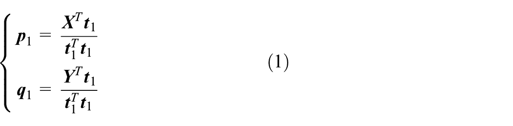
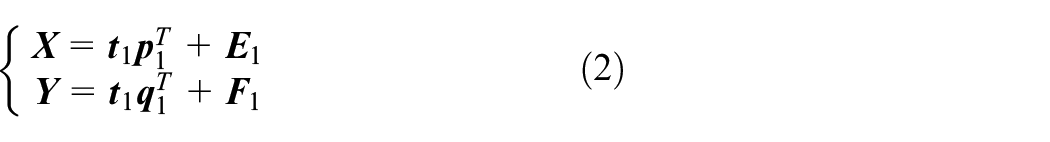
We treat
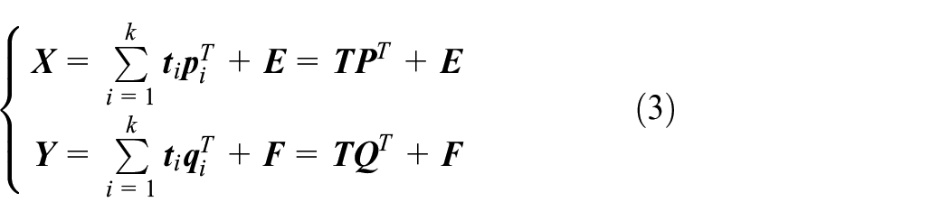
To establish the relationship between
Two matrices,

FNN and AE
FNN has only one hidden layer, which is fully connected with the input and output layers. No connection exists between the nodes of two layers that are not adjacent or between nodes of the same layer. The hidden layer has the maximum number of nodes,
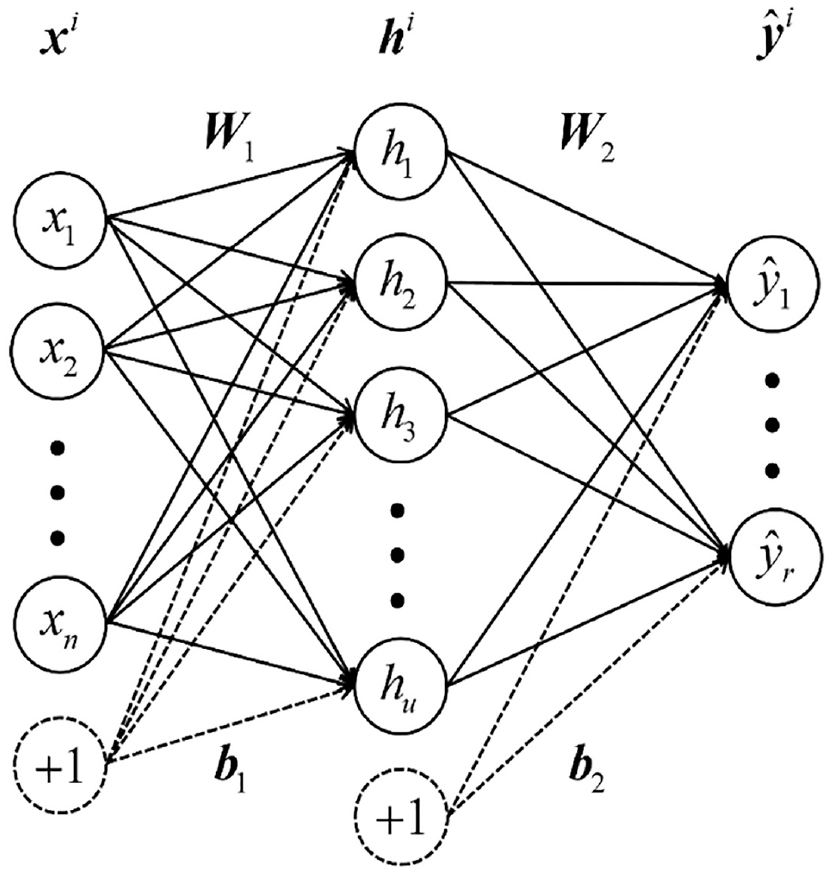
FNN structure.

where
AE is an FNN with a special structure that is widely used in unsupervised learning. First, its input and output layers are of the same sizes because the output needs to be the same as the input. Second, the hidden layer has the least number of nodes because its target is to extract features. The BP algorithm is also used for training the network.
Fault detection based on PLS-DFNN model
The structure of our DFNN is specially designed to imitate PLS. Thus, first, we detail its construction process. Second, we introduce the decomposition of subspaces based on our model. Third, we provide the calculation of monitoring statistics and threshold determinations. Finally, we show the entire scheme of fault detection.
DFNN structure
The construction of DFNN can be divided into four steps. Figure 2 is the diagram of each neural network. We initially construct a simple FNN with the assumption that the input is
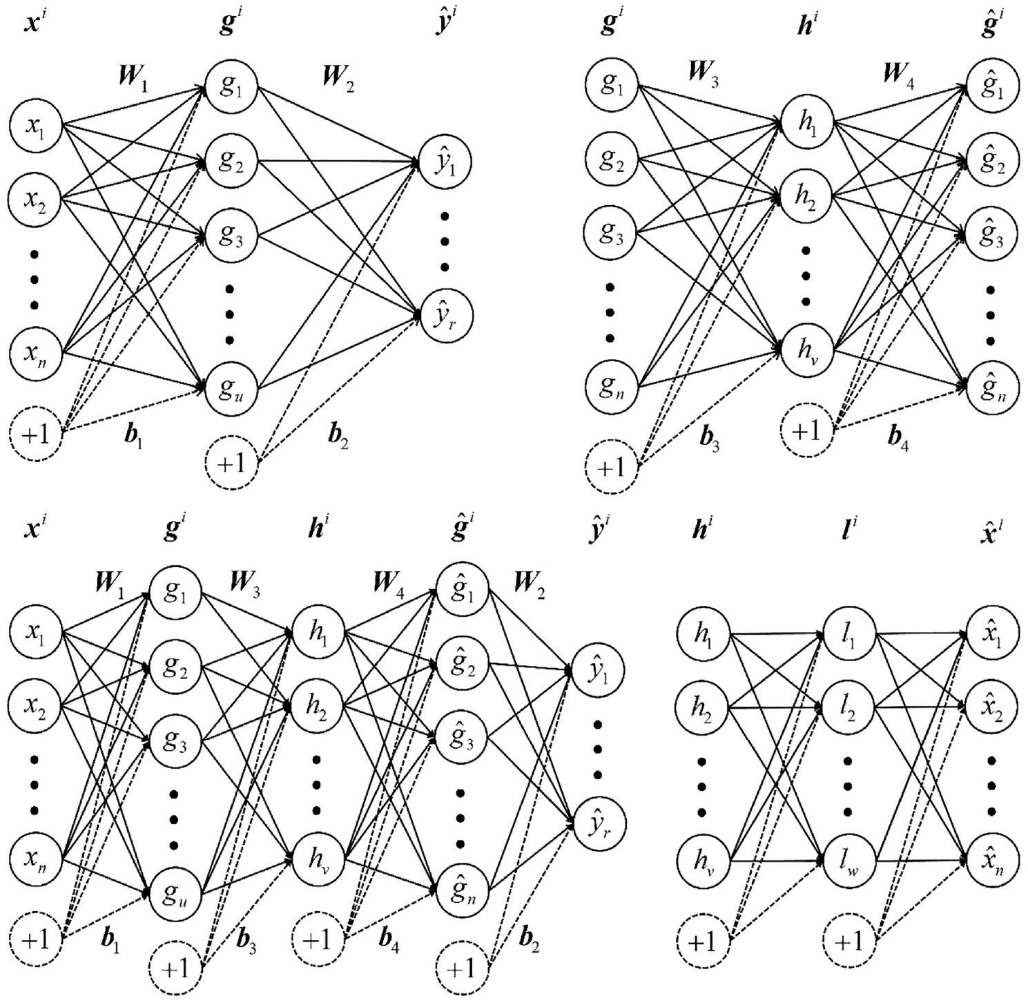
DFNN structure.
Subspaces based on PLS-DFNN
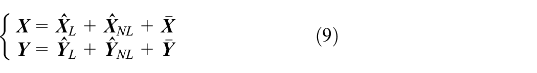
First, process variables

Subscript L is the linear estimation, and
Residual spaces
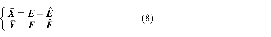
We view
Monitoring statistics and threshold determinations
We assume that only process variables can be obtained during online monitoring. Quality variables will be delayed. Thus, we use them to verify the monitoring results. We set three statistics to monitor the three subspaces of
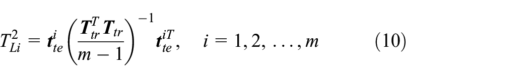
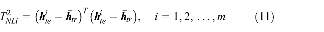
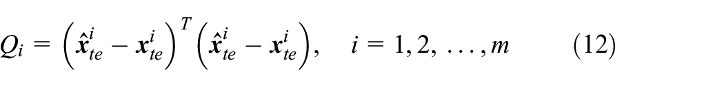
where subscripts tr means the offline training samples and te means the online testing samples.
We monitor the quality variables similarly as equation (10) to verify the results. The monitoring statistic is written as
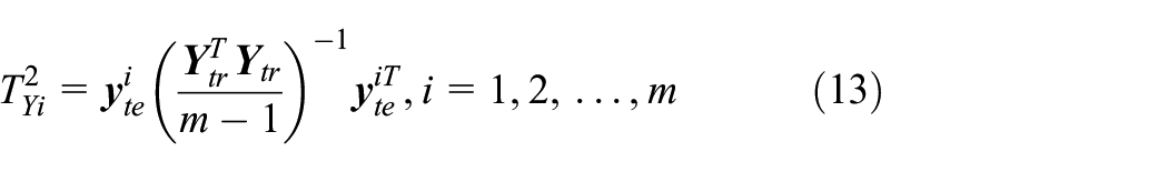
where
The kernel density estimation (KDE) method (Chen et al., 2000; Gonzalez et al., 2015) is used to calculate threshold determinations. On the basis of the distribution of
When the monitoring statistics are calculated in online monitoring, they will be compared with threshold determinations. The samples with larger statistics than threshold determinations will be judged as a fault. If we can study prior knowledge before testing, then we can obtain the relationship between fault and quality to choose the correct monitoring statistics.
Scheme of fault detection
The detailed scheme of the proposed approach is shown in Figure 3. The implementation contains offline modeling and online monitoring. The detailed steps are summarized as follows:
Offline modeling:
Step 1: Normalize process and quality variables and save the parameters.
Step 2: Use PLS to extract linear features to obtain PLS dominant space and residual space.
Step 3: In PLS residual space, use DFNN to extract nonlinear features to obtain DFNN dominant space and residual space.
Step 4: Use formula equations (10)–(13) to obtain
Online monitoring:
Step 1: Use offline modeling parameters to normalize online process variables.
Step 2: Obtain
Step 3: Generate the detailed information when a fault occurs.
Because linear and nonlinear relationships may be difficult to distinguish in most cases, we design an “OR” logic as
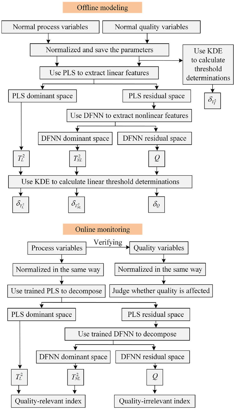
Architecture of PLS-DFNN fault detection.
Experiments and discussion
Before our model is applied to FCC process, we test our model on two data sets. The first data set is a numerical simulation data set, and we prove the capability of our model to detect linear quality-relevant, nonlinear quality-relevant, and quality-irrelevant faults. The second data set is the TE process data set, and we compare our detection results with those of other related models to show the superiority of our model.
Numerical simulation data set
We initially set seven original variables

Second, the process variables are the product of original variables and random matrix in equation (15).
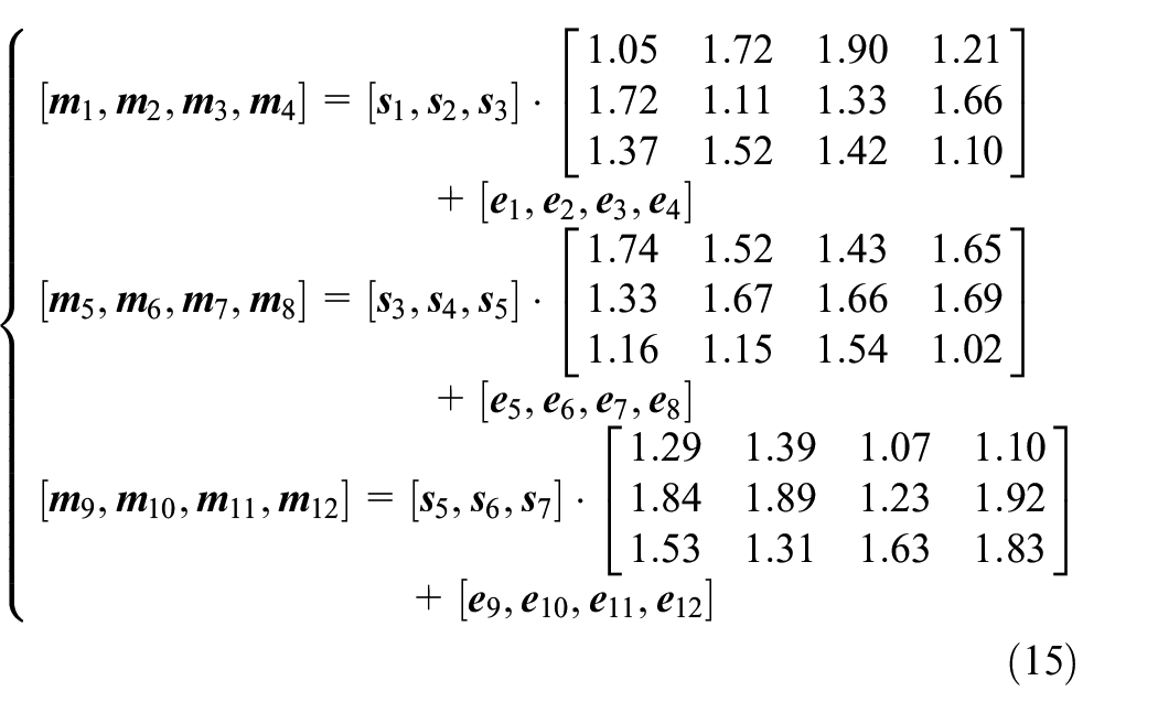
Third, we establish the quality variables according to equation (16).

The first two quality variables have a linear relationship with process variables, and the last two have a nonlinear relationship. Other process variables have nothing to do with quality.
Our training set is as described above, and then, we start to obtain the testing sets by adding different noises to the process variables and set up different faults starting from the 201st sample. We set up three step changes with amplitudes of 0.04, 0.07, and 0.05 on
Extracting linear features by PLS
We want PLS to extract two components because we have two quality variables that have a linear relationship with process variables. If the two features can perfectly represent the two quality variables, then the project matrix should be equation (17). The actual project matrix is equation (18).
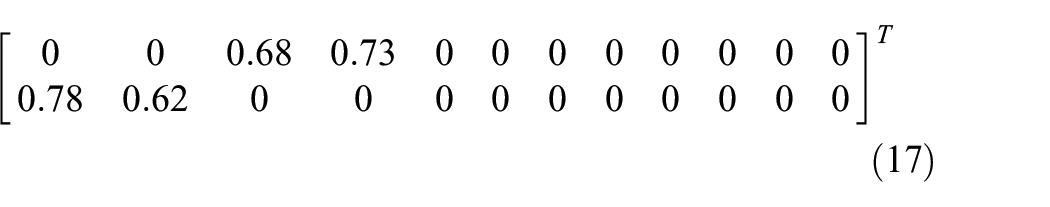

The results are close, which proves the effect of PLS. Then, we calculate residuals
Extracting nonlinear features by DFNN
The structures of two DFNNs that estimate
Detecting results of three testing sets
We decide k by 10-fold cross-validation. The
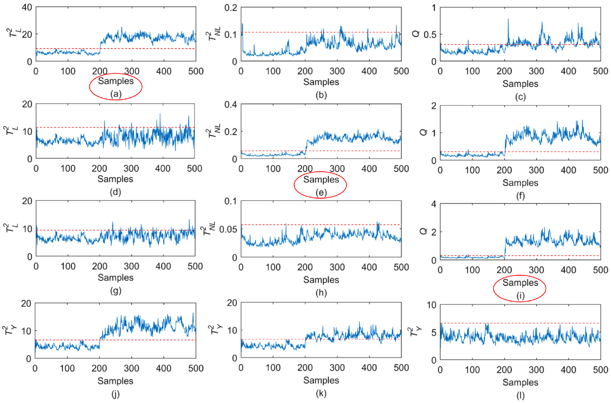
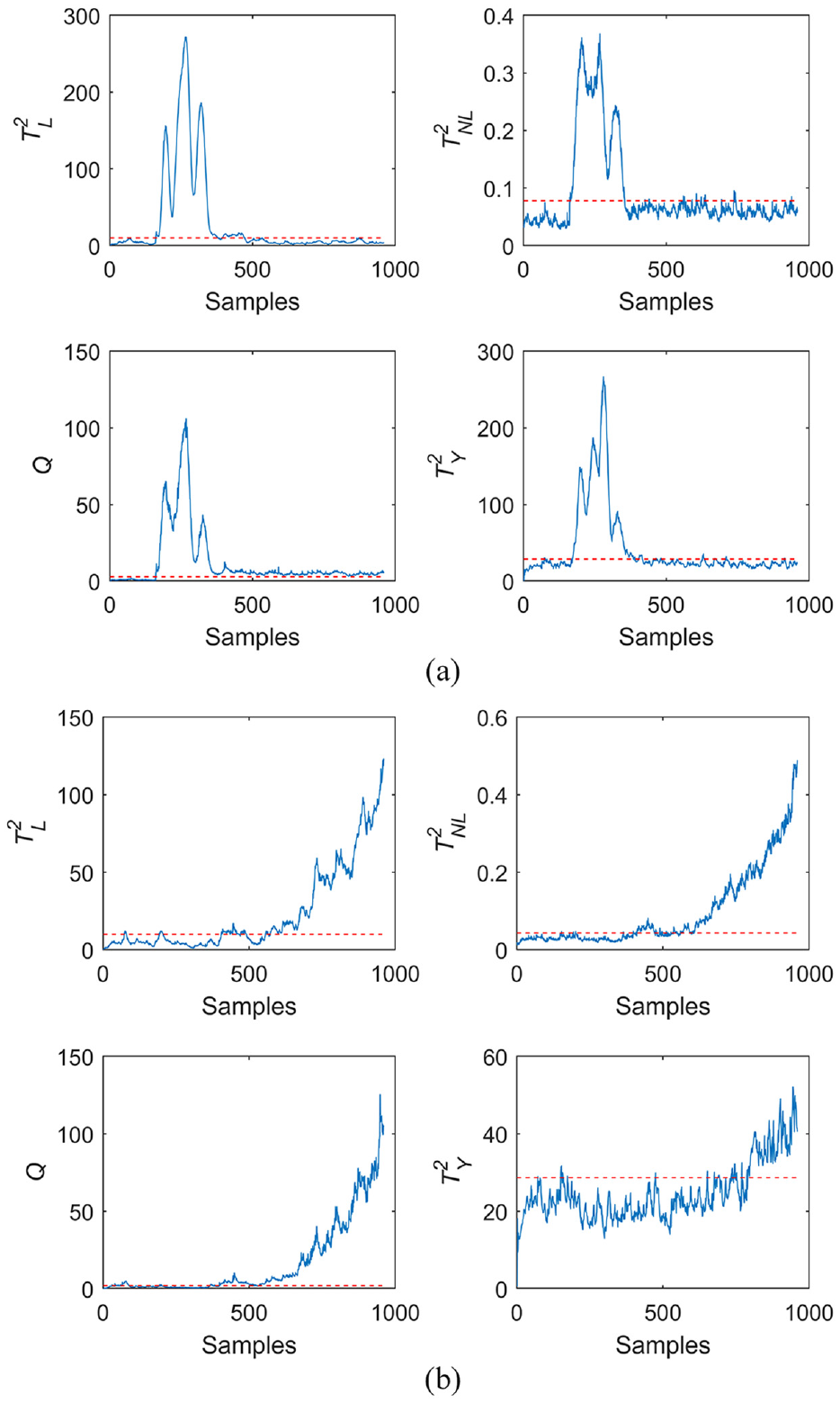
Detection results of the numerical simulation data set: (a)–(c) Fault 1. (d)–(f) Fault 2. (g)–(i) Fault 3. (j)–(l) Verifying.
We calculate the false alarm rate (FAR) and the fault detection rate (FDR) as the standard to evaluate the performance of the model. Table 1 shows the results. The first fault occurs on
FAR (%) and FDR (%) of three monitoring statistics on three faults.
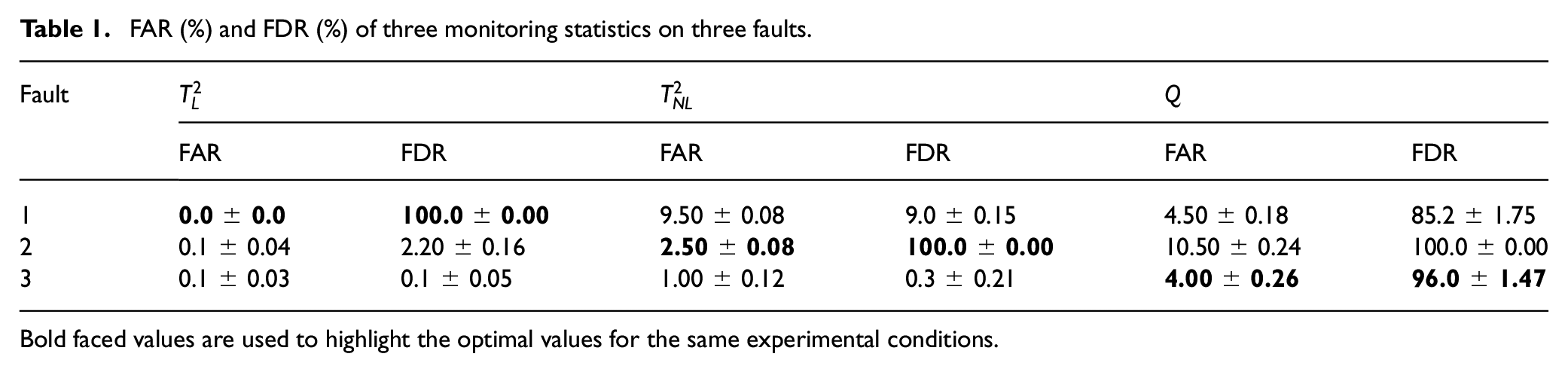
Bold faced values are used to highlight the optimal values for the same experimental conditions.
Verification
The last line of Figure 4 shows the statistic
TE process data set
TE process simulates an actual chemical program. A total of 52 variables are set up in simulation, and they comprise 33 process variables that can be obtained in real time and 19 quality variables that must be analyzed (Downs and Vogel, 1993). The former is directly detected by process instruments; thus, they become
Faults of TE process data set
Chiang et al. (2000) improved the simulation process and sorted out 22 data sets, including normal condition, and 21 faults. Prior knowledge can provide great help for fault detection. We can classify those faults based on the description of each fault (Kong et al., 2018; Li et al., 2019; Wang and Jiao, 2017). Faults 1, 2, 5, 6, 7, 8, 10, 12, 13, and 21 are quality-relevant, and
Each of the 22 training sets has 500 samples, and each of the 22 testing sets has 960 samples. Our model is trained based on the normal training set and is tested on 21 fault testing sets. Those fault testing sets are particularly designed because the fault appears from the 161st sample; in this manner, FAR and FDR can be comprehensively examined.
Model establishment
When establishing the PLS model, we decide k by 10-fold cross-validation. The prediction error is minimized by the principle of
The DFNN structures are 33-45-29-45-19 and 29-31-33. The maximum training epoch is 5000, and the accuracy requirement is 0.01. All of these factors are decided according to experience.
Fault detection and verification
We give FAR and FDR of all faults under
FDRs (%) of seven methods on TE process data set.
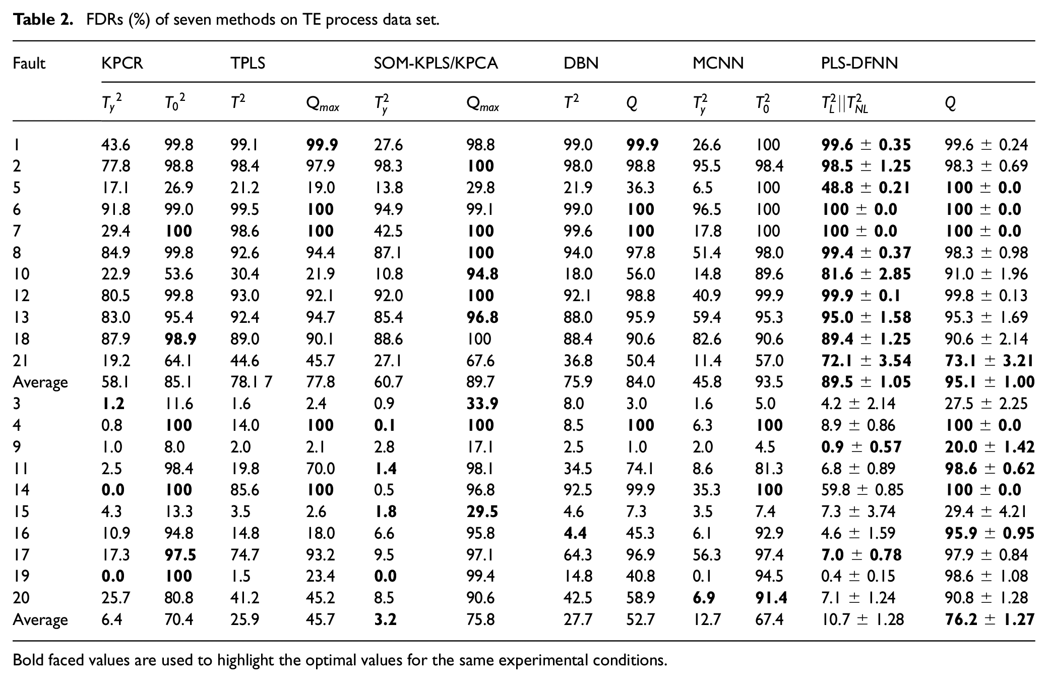
Bold faced values are used to highlight the optimal values for the same experimental conditions.
According to the FDR of
Figure 5 shows the result of Faults 5 and 21. The quality for Fault 5 is only affected for a period of time after the fault occurs, and then, it quickly returns to normal.
Detection and verification of results in TE process data set: (a) Fault 5 and (b) Fault 21.
Generally, our method effectively distinguishes quality-relevant and quality-irrelevant faults, which also reflects the rationality of decomposing the subspaces. Our method also provides better monitoring performance than the other methods.
Applications on FCC process
In this section, PLS, DFNN, and PLS-DFNN are applied to an actual FCC process, and their performance in process monitoring is analyzed and compared. All production data are derived from the FCC unit of a petrochemical enterprise in Beijing. The characteristics of the three methods above are compared and discussed using the data of the whole year in 2020.
FCC process
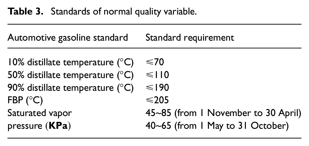
FCC unit is a secondary refining unit with heavy oil as raw material. The main products are dry gas, liquefied petroleum gas (LPG), gasoline, diesel, and slurry (Ancheyta et al., 2004; Han and Chung, 2001; Lin and Zeng, 2013; Vistisen and Zeuthen, 2008). The main unit consists of a reaction regenerator, a fractionator, two absorption towers, and a stabilizer tower. The flow chart is shown in Figure 6. After entering the unit, the raw material is preheated first and then sent to the reaction system for catalytic cracking reaction. The reaction oil and gas are sent to the fractionation system for separation to obtain crude products such as gasoline and diesel. The rich gas and crude gasoline at the top outlet of the fractionator enter the absorption and stabilization system for further separation to obtain dry gas, LPG, and stabilized gasoline (Chang et al., 2014; Naik et al., 2017; Wang et al., 2016a). Among these products, gasoline is the most important and the most productive fraction. Therefore, producing qualified gasoline is important for FCC process (Han and Chung, 2001). ASTM D86 and saturated vapor pressure are two important indexes of vehicle gasoline, and they reflect the evaporation performance of gasoline. The difficulty of gasoline engine starting is determined by 10% distillate temperature. A total of 50% distillate temperature determines the heating and acceleration times of gasoline engine. A total of 90% distillate temperature and final boiling point (FBP) determine whether gasoline can be completely evaporated and burned. Saturated vapor pressure determines the start-up loss of gasoline engine and plays an important role in the environment (Gupta et al., 2007). However, these data cannot be detected online in real time due to the difficulty of measurement and the inability of remote transmission of some instruments. In addition, we prefer to use process variables to reflect whether and what type of fault occurred in production conditions. Therefore, the data-driven method has more advantages.
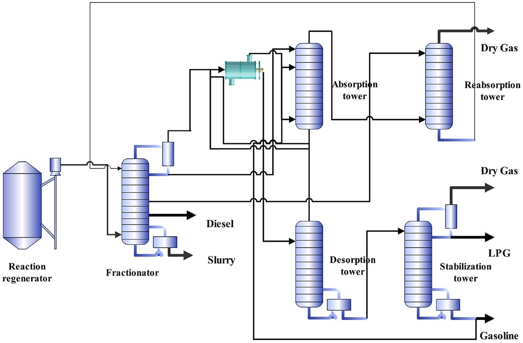
Flow chart of catalytic cracking process.
Fault detection of FCC process
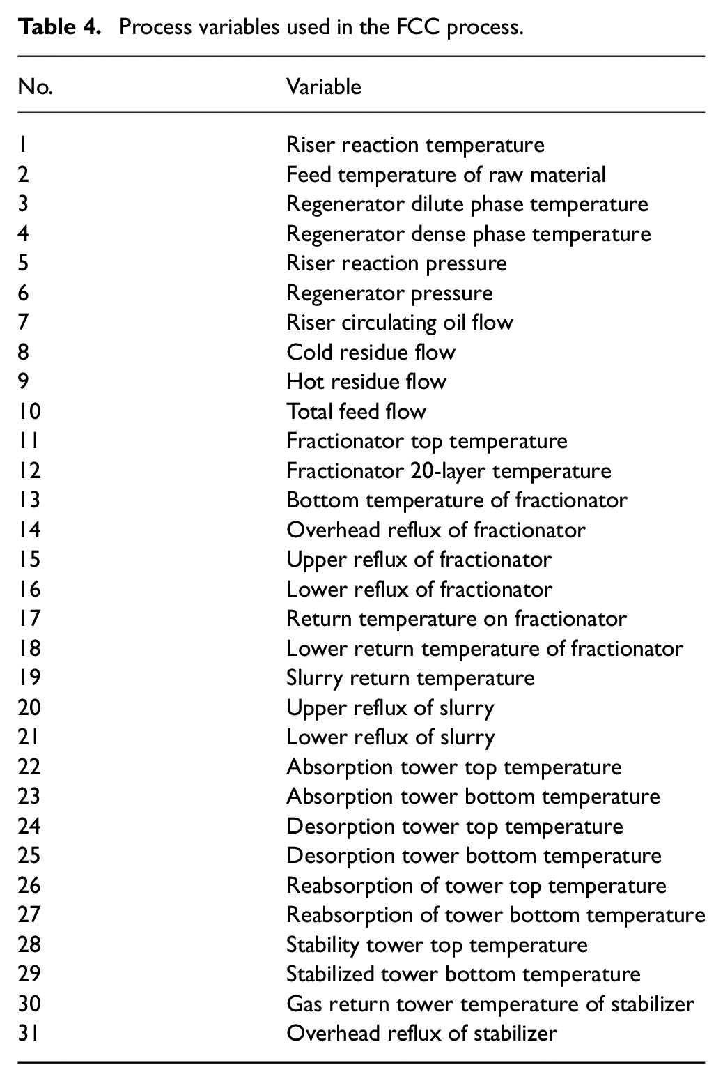
According to the latest national standards for automotive gasoline, ASTM D86 and saturated vapor pressure should meet certain requirements, which are displayed in Table 3. The FCC process has failed when the produced gasoline does not meet these standards. We collected the data of the whole year in 2020, and 31 process variables can be used for state detection, as shown in Table 4. Quality variables are unconventional monitoring data. Thus, the data scale that can be collected is limited. After comprehensive consideration, 50% distillation temperature, FBP, and saturated vapor pressure are finally selected as quality variables. The saturated vapor pressure data are those on 1 May and solstice on 31 October. Given that ASTM D86 distillation curve and saturated vapor pressure are not measured simultaneously, we consider them as quality variables separately.
Standards of normal quality variable.
Process variables used in the FCC process.
Faults of FCC process
According to the technical monthly report, the fault was caused mainly by the riser reaction temperature fluctuations. Faults have different effects on the three quality variables of 50% distillate temperature, FBP, and saturated vapor pressure, and the collected data correspond to different times. Thus, they can be regarded as three groups of faults, which are respectively called Faults 1, 2, and 3. Each training set consists of 500 samples. Table 5 lists the types of faults for the testing set and the number of samples where the faults occurred and ended. The fault types can be divided into quality-relevant and quality-irrelevant according to their influence on quality variables.
Description of the faults.
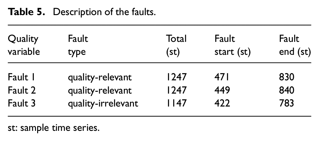
st: sample time series.
Performance of PLS
We use 10-fold cross-validation to determine the number of components in PLS. Table 6 lists the prediction errors of selecting different quantity components for each fault. For the three kinds of faults, the prediction error is less than that in other cases when
Cross-validation in PLS on the FCC process.
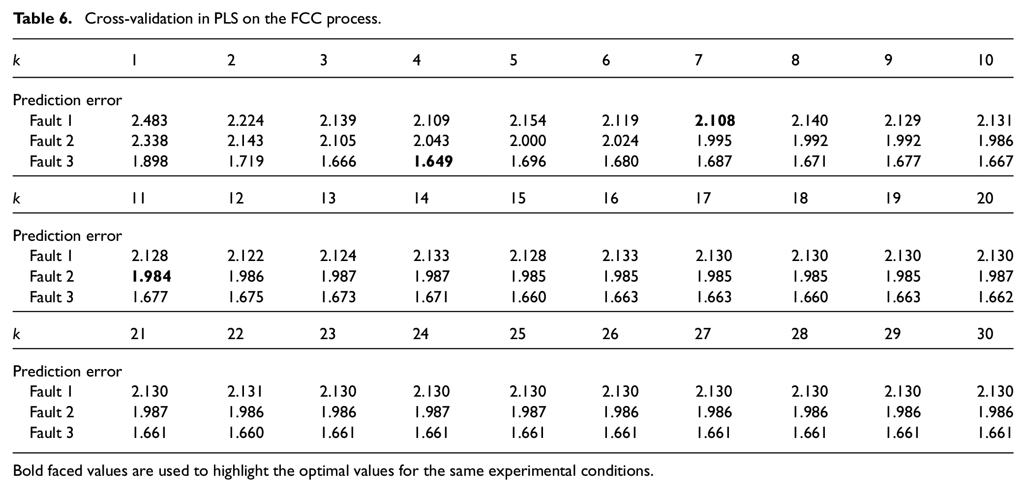
Bold faced values are used to highlight the optimal values for the same experimental conditions.
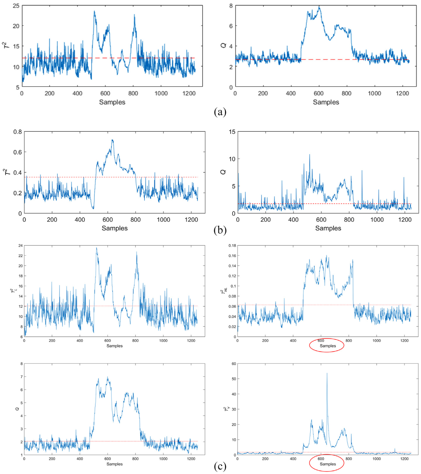
Detection results of the FCC process on Fault 1 by (a) PLS, (b) DFNN, and (c) PLS–DFNN.
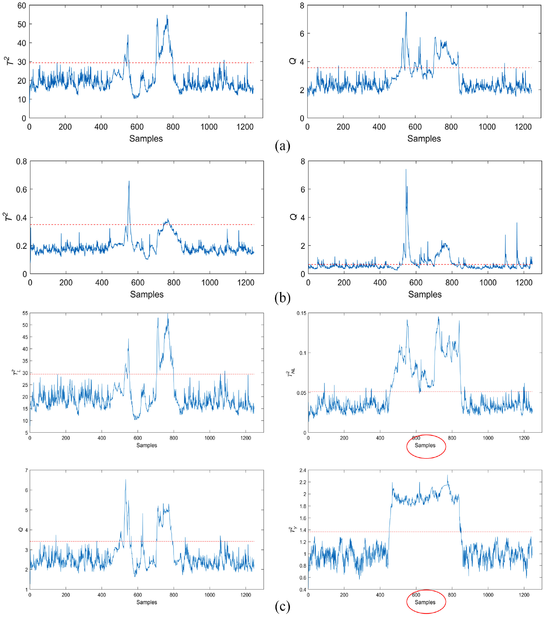
Detection results of the FCC process on Fault 2 by (a) PLS, (b) DFNN, and (c) PLS–DFNN .
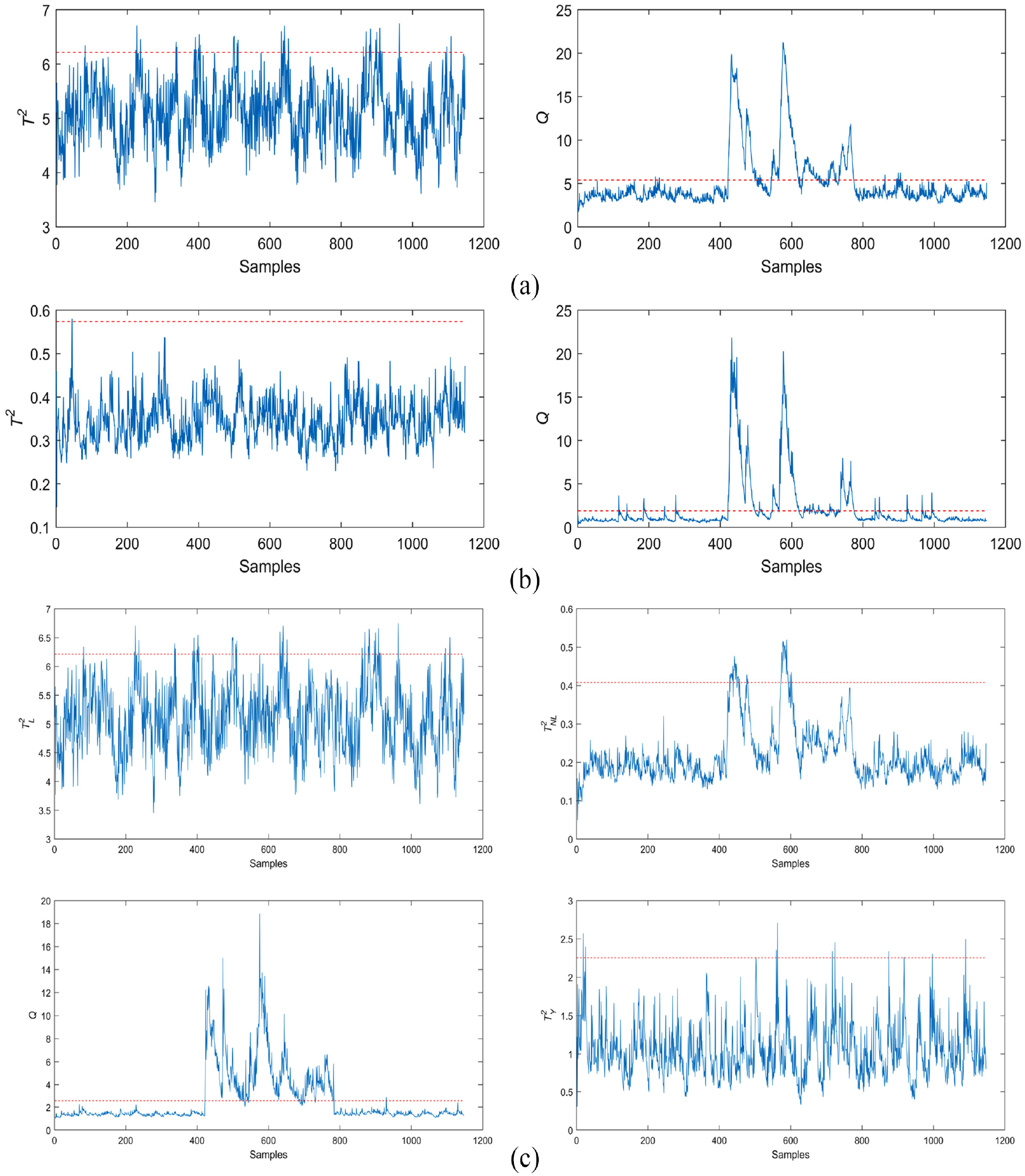
Detection results of the FCC process on Fault 3 by (a) PLS, (b) DFNN, and (c) PLS–DFNN.
Performance of DFNN and PLS-DFNN
We keep the structures of DFNN consistent as 31-55-12-55-1 and 12-20-31 to test the performance of DFNN and PLS-DFNN. The maximum training epoch is 5000, and the accuracy requirement is 0.01. Figures 7(b), 8(b), and 9(b) are the results of DFNN corresponding to three kinds of fault detection. Meanwhile, Figures 7(c), 8(c), and 9(c) are the results of PLS-DFNN. Comparison statistics of the detection performance of the three methods are shown in Table 7. Through
FARs (%) and FDRs (%) of three methods on the FCC process.
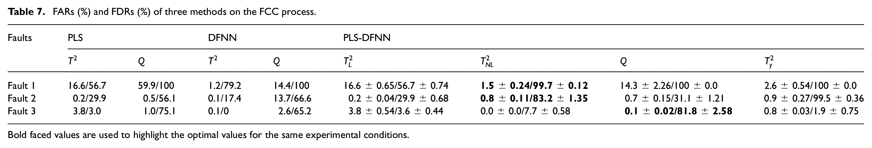
Bold faced values are used to highlight the optimal values for the same experimental conditions.
Conclusion
We propose PLS-DFNN to effectively monitor the quality of FCC process. From the perspective of linearity and nonlinearity, we decompose three subspaces for further extracting information from variables. We prove that three monitoring statistics for three subspaces of PLS-DFNN can excellently monitor three types of faults. However, the specific division of three subspaces depends on the number of components of PLS that are determined by cross-validation and the network structure that is determined by experience. An improved division method can be further studied, and the performance may also be further improved.
We can choose the appropriate monitoring statistic for the fault on the basis of the detection of quality variables. PLS-DFNN provides good performance on the TE process data set and the FCC process.
Footnotes
Appendix A
Declaration of conflicting interests
The author(s) declared no potential conflicts of interest with respect to the research, authorship, and/or publication of this article.
Funding
The author(s) disclosed receipt of the following financial support for the research, authorship, and/or publication of this article: this work was supported by the National Natural Science Foundation of China (grant no. 21878081).