Sage Journals: Discover world-class research

Abstract

While police officers must adapt behavior between places to effectively do their jobs, these decisions could result in some communities receiving different levels of exposure to the police. This study explores a new spatial measure of police contacts to observe these differences. We calculate neighborhood-specific Gini coefficients based upon the spatial distribution of 77,752 police-civilian stops at street segments and intersections nested within census tracts in Oakland, California. This coefficient presents a contrast between two divergent distributional patterns—the diffusion of police contacts to more places across neighborhoods and the concentration of contacts at fewer “hot spot” places within neighborhoods. The most consistent environmental explanation for these differences was the race/ethnicity of neighborhood residents, which was associated with the police stopping people across more places. Future research should continue to investigate this finding and examine the mechanisms that explain why spatial exposure to police contacts changes between places.

Keywords

police contacts police behavior neighborhood effects hot spots race

The police are a public-facing symbol of the government’s authority in the United States and are often considered the gatekeepers of the criminal justice system. In 2020, over 53 million Americans had direct contact with the police with just under half of those contacts initiated by police officers (Tapp & Davis, 2022). Contemporary research has established the process by which people are treated in these interactions by police officers is often more influential than the outcome of the interaction (see Tyler, 2004). These contacts shape individual’s perceptions of police legitimacy and broader trust in government authority, which influence the general safety of communities and an individual’s willingness to cooperate with the police. Due to these far-reaching implications, police-civilian contacts matter and represent a critical juncture to examine the impact of the criminal justice system on communities.

There are two main ecological explanations for why some locations could receive varying numbers of police contacts and different levels of exposure compared to other places (see Klinger, 1997). For instance, the spatial distribution of police contacts is influenced by land use and crime reporting. The police are more likely to make contact in locations where there are more people, facilities, and public spaces (Brantingham & Brantingham, 1991). Police agencies have become more reliant on using data-driven strategies such as CompStat and hot spot policing, which efficiently channel resources to locations that experience the most crime within cities. In contrast, substantial literature exists that suggests the police might engage in different patterns of contact at places based on the socio-demographic characteristics of a places’ residents such as race/ethnicity and economic status (see Brunson, 2007). As a result, these communities could experience either over- or under-policing due to the spatial concentration of these disadvantaged social groups at locations (Boehme et al., 2020).

This study explores a novel approach to measure the spatial distribution of police-civilian contacts and tests the effectiveness of these traditional ecological perspectives to explain differences between places. Our analyses examine neighborhood-specific Gini coefficients to observe the distribution of police contacts at the micro-places nested within these locations (see O’Brien et al., 2021). These coefficients contrast two divergent possibilities: (1) there is more concentration of police stops between micro-places within neighborhoods or (2) there is more diffusion of stops between micro-places within neighborhoods. This study contributes a new dimension to explore differences in police practices between places. Therefore, moving beyond using just the frequency of contacts at places (i.e., counts) to quantify the underlying geographic footprint or spatial exposure of communities to contacts from the police. In other words, a neighborhood where the police contact civilians across a wide range of places is materially different from a neighborhood where the police only contact civilians in a few specific places.

This study examines a core debate about policing by conducting an exploratory test of the effectiveness of traditional ecological perspectives to explain the spatial variability of these distributional patterns. Are differences in distributional patterns of police contacts between places explained by routine police work (e.g., cops follow crime reporting) or the social characteristics of places (e.g., race/ethnicity influences decisions)? In the aftermath of the death of George Floyd, there has been renewed public attention toward the intersecting topics of race and policing. Some scholars have since engaged in a critical reexamination of the central tenets of policing such as whether differences in police behavior across places is the byproduct of perpetuating a systemic bias against disadvantaged communities and not just routine police work (see Bolger et al., 2021). Our analyses conduct a limited but insightful test of these divergent ecological perspectives on differences in police behavior between places to contribute more evidence to this on-going debate. This study helps inform discourse around this salient topic in criminal justice and advances criminological theory by providing preliminary insight into why some neighborhoods receive different levels of spatial exposure to police contacts compared to others within urban areas. In addition, the findings from our study can further strengthen criminal justice policies constructed around either promoting the positive aspects of police contacts or mitigating the negative aspects of these contacts.

Police Contacts and Place

Overview

Police officers must adapt behavior between places to be responsive to the disparate needs of communities. There is extensive literature on the influence of place on police contacts. Police contacts are a general concept that includes any possible interaction between a police officer and a civilian (Tapp & Davis, 2022). An overwhelming majority of these contacts do not result in the most invasive outcomes such as a search, arrest, or use of force. Most research on neighborhood context and police contacts has focused on traffic and pedestrian stops (see Huff, 2021). Klinger (1997) proposed an influential theoretical model that integrates individual-level decision-making processes of officers with broader ecological factors such as neighborhood crime rates to demonstrate how police behavior changes between places. Previous research has demonstrated that neighborhood context may influence police contacts such as the use of force (Terrill & Reisig, 2003). Other research has examined whether neighborhood characteristics impact community perceptions and satisfaction with the police (Boehme et al., 2020). Some recent studies have extended this research to systematically observe a wide range of police behaviors at micro-places within neighborhoods (see Nouri, 2021).

Ecological Perspectives

In general, the “routine police work” and “social characteristics” hypotheses are the two most common explanations for why police contacts could vary between places. Police behavior varies between places as a regular function of police work. Patrol is often considered the “backbone” of police work and one of the primary sources for officer-generated police-civilian contacts. Over the last 50 years, there has been a seismic shift from police agencies using routine preventive patrol across all places within jurisdictions to more focused patrols at a smaller number of crime-prone places. The Kansas City Preventive Patrol experiment (Kelling et al., 1974) provided a landmark critique of the benefits of routine preventive patrol on crime control across all places, and a substantial empirical foundation has since emerged on the benefits of using more directed hot spots policing strategies (Weisburd & Braga, 2019). The popularity of organizational management systems like CompStat provided further dependence on quantitative analytics to guide resource allocation pertaining to patrol (i.e., CompStat is short for “compare stats”). Today, police agencies are also exploring predictive policing models of resource allocation.

Another primary source of police contacts is civilian-generated calls for service. Depending on call volume and the specific calls received, the police might reactively spend more time in certain communities. Therefore, the police spend time where the public calls them, or police behavior could vary between places because of workload. There is much conflicting evidence on the effect of police contacts on communities. Some research suggests that when police officers engage in community-oriented policing techniques, these contacts can have a lasting positive effect on individuals (Gill et al., 2014). Community-oriented policing may require a greater police presence in certain locations (Adams et al., 2005), but this presence is associated with increased public satisfaction with police, improved perceptions on neighborhood disorder, enhanced police legitimacy, and/or reduced fear of crime (also see Gill et al., 2014). Some scholarship finds that “quality” contacts (e.g., contacts that result in a fair outcome) with police may in fact improve perceptions of police (see Skogan, 2005). Furthermore, the benefits of a greater police presence may improve the overall social control of the neighborhood and civilian’s willingness to report crime.

In contrast, police behavior may vary between places because of the social characteristics of these locations. There is a long history of research and public perception of biased treatment from the police against disadvantaged communities (see Weitzer & Tuch, 2006). There are often racial/ethnic disparities in police-civilian contacts (Foster et al., 2022), and recent high-profile use-of-force encounters have served as rallying cries to further consider this perspective on police behavior. Some research suggests members of disadvantaged communities often do not feel as comfortable calling the police, which would indicate these places could experience lower levels of policing (Carr et al., 2007). The concepts of over- and under-policing have become generally applied to organize thought on these more specific issues (Crowther, 2013). The former suggests the police have a larger presence at places based on sociodemographic characteristics of residents and engage in more police-civilian contacts, which results in these disparities. The latter suggests the police do not respond to certain communities and divest resources from these places which provides a type of neglect to these locations.

Rios (2011) conducted an influential ethnography of Black and Latinx youths and their experiences with the police in Oakland, California. This study highlighted how Black and Latinx neighborhoods are simultaneously over-policed (e.g., targeted and disproportionate arrests) and under-policed (e.g., neglected and ignored), both of which negatively impacted the well-being of such communities. Furthermore, Rios argues youths from these neighborhoods are consistently targeted and harassed by the police at an early age, which comes with a wealth of adverse outcomes such as social exclusion, expulsion from schools, and a lack of prosocial opportunities throughout adulthood. Even outside of these diverse communities, the race-out-of-place literature suggests that when the race/ethnicity of a civilian does not align with the majority composition of a neighborhood, this may draw greater suspicion and likelihood of contact from the police. Some studies have found that people of color may be more likely to be stopped and questioned in a predominantly White neighborhood (see Carroll & Gonzalez, 2014).

While there can be undeniably positive effects of police contacts, most research has critically focused on the negative effects of police-civilian encounters. Some research suggests contacts with police officers may negatively affect individual’s perceptions of the institution of policing (Slocum & Wiley, 2018), with frequent contacts strongly influencing these negative perceptions and increasing perceptions of being profiled or targeted (Weitzer & Tuch, 2006). While police are largely held in high regard by the public, these perceptions often vary by the race of the civilian, as people of color tend to hold more negative perceptions of police in comparison to their White peers (Braga et al., 2019). The present study does not presuppose police-civilian contacts are inherently positive or negative; instead, we just emphasize differences in their spatial distribution between places, which is meaningful to observe for the sake of criminological theory and criminal justice policy.

The Present Study

The goal of the present study is to explore the spatial distribution of police contacts using Gini coefficients and further understand how neighborhood ecological characteristics influence variability of these spatial patterns. Overall, there are three main contributions of this present study. First, we present a new dimension to study spatial patterns of police contacts with our methodological approach focused on Gini coefficients. This study offers the first known analysis to apply Gini coefficients to explore the spatial distribution of police-civilian contacts. We propose that research should address the critical distinction of not just the number of police-civilian contacts at places but also where they occur across places and how police behavior varies between places. These coefficients present two distinct ecological portraits or profiles. For instance, the diffusion of police contacts across a wide number of places suggests a broader neighborhood-based impact while concentration of contacts presupposes more of a micro-level or “hot spot” effect.

Second, this research design helps enhance conceptual and theoretical understanding of the mechanisms that explain differences in police behavior between places. This contrast between micro-places and neighborhoods is critical to contemporary research to determine the unique effect of each unit of analysis or spatial scale when constructing integrated place-based theories. In other words, the focus of spatial inquiries on police practices should be more centered on understanding decisions made at a few specific micro-places or, more generally, across neighborhoods. The examination of these patterns provides a window into the psychology of policing and the decision-making processes of both officers on patrol and police leadership. Specifically, what characteristics of places influence why the police stop civilians in more or less micro-places within neighborhoods, and are these patterns ecologically independent?

Our analyses can provide preliminary evidence to suggest whether differences between places are explainable by simple factors such as the routine police work hypothesis or more complex realities such as the social characteristics hypothesis. Third, our analyses have policy implications to improve police–community relationships based on the factors that emerge from our analysis as salient explanations of the exposure to police contacts. Specifically, the deployment of policing strategies that promote the positive aspects of certain police contacts (e.g., community policing) or reduce the impact of the negative aspects of other contacts (e.g., procedural justice policing). These contributions are timely due to the increased public discourse on police legitimacy in the aftermath of high-profile use of force cases.

Data and Methods

Oakland and Police Stops

We examined all civilian stops conducted by the Oakland Police Department (OPD) from January 1, 2017, to December 31, 2019.¹ We accessed these records through a public data request via the city of Oakland’s public data portal.² This data represents a general measure of police contacts, which includes any traffic or pedestrian stops of civilians. OPD officers are required to officially document every substantive contact with civilians regardless of whether the interaction leads to formal processing such as a citation or arrest. These contacts are sometimes referred to as “field interrogations.” For instance, these contacts capture all individuals who had noncustodial police contact, were searched, had a quality-of-life violation, and were arrested (see Papachristos et al., 2015). Stops have been repeatedly used in previous research to examine the characteristics of police-civilian contacts (Tapp & Davis, 2022). We analyzed stops pooled across three years to minimize the influence of any outlier years, observe more spatial variance, and assess the last extended period before the COVID-19 pandemic began (i.e., March 2020). There were 78,894 recorded stops across our three-year observation period.³

We examined two nested spatial units of analysis within Oakland. Census tracts (n = 113) were used as a proxy for neighborhoods, and we developed “street units” (n = 16,464) to represent micro-places. Due to OPDs recording procedures for stops, there were two main considerations that influenced our selection of these micro-spatial units of analysis. First, OPD officers were only instructed to record stops to 100 blocks of addresses instead of precise street addresses (i.e., 123 Main St. becomes 100 Main St.). Second, OPD officers were also permitted to record the location of stops at street intersections in addition to 100 blocks. Therefore, we developed street units as our micro-place unit of analysis, which combines street segments and intersections to account for these considerations of how OPD collected data on police stops (see Braga et al., 2010). In general, most street segments in Oakland corresponded to 100 blocks of addresses. All spatial calculations were conducted using ArcGIS 10.8, and base maps were collected from Oakland’s public data portal. The final geocoding rate was 98.6% (77,752 of 78,894), which far exceeds the 85% threshold suggested by Ratcliffe (2010) for high assignment accuracy. Our final dataset included 77,752 stops and identified 16,464 street units nested within 113 census tracts (see Online Supplemental Material).

Gini Coefficients

We adopted the methodology outlined in O’Brien et al. (2021), which pioneered the use of these measures to observe the distribution of crime incidents. Our application to police contacts provides a noteworthy contrast, shifting from loosely connected civilian-generated behaviors to assessing police officers’ more interconnected behaviors as representative of the broader criminal justice system. Gini coefficients are a summary descriptive measure that has become commonly applied due to critiques of the law of crime concentration (see Weisburd & Braga, 2019) and using arbitrary distributional thresholds. The Gini coefficient provides a more comprehensive, standardized scale to measure inequality, which is commonly used across other disciplines such as economics. In turn, a neighborhood-specific Gini coefficient is a quasi-hierarchical measure with our analysis using level 1 as street units and level 2 as census tracts.

This measure considers both the number of stops found within neighborhoods, the number of street units across the neighborhood that experienced stops, and the distribution of stops between these street units. These coefficients provide a synthesis of complex hierarchical and spatial features of data into a parsimonious value. These coefficients present a continuous variable ranging from 0 to 1, which assesses distributional concentration (see the Online Supplemental Material for the equation). Values closer to 0 indicate an even distribution of stops across street units within tracts. In contrast, values closer to 1 indicate a completely uneven distribution characterized by all stops concentrated in a small number of street units. Thus, the contrast between these two axes from Gini coefficients comments on the unit of analysis or scale, which is most helpful to understand the exposure to police contacts. To further demonstrate, consider a neighborhood with both 100 micro-places and 100 stops. If the neighborhood has all 100 stops found within 1 micro-place, this would represent the highest level of concentration with a Gini coefficient of 0.99. If the neighborhood had 100 stops evenly distributed across 50 micro-places (i.e., 2 per micro-place), the coefficient is 0.50. Finally, if the neighborhood had all 100 stops evenly distributed across all 100 locations, the coefficient is 0.00. Despite the identical number of stops and micro-places, where these stops occur and how they are distributed reveals a critical dimension to understanding the true exposure of places to contacts.

These values represent the ratio of the area between the line of perfect equality and the observed Lorenz curve to the area between the line of perfect equality and the line of perfect inequality (Schnell et al., 2017). In our case, Lorenz curves plot the cumulative percentage of street units against the cumulative percentage of stops within neighborhoods. A generalized Gini coefficient was developed to address a common limitation of place-based research, which is that there are often more places than crimes observed (Bernasco & Steenbeek, 2017). Therefore, these calculations are adjusted to account for a different line of equality, which reduces estimates of concentration by contrasting stops to only the number of places they could be reasonably distributed between. For example, if a neighborhood has 50 stops but 100 total street units, the true 0-value of a completely even distribution across units is not possible to achieve.

All Gini coefficients were calculated in R using the lorenzgini package (Steenbeek & Bernasco, 2018). We calculated the standard Gini coefficient and generalized coefficient to contrast the results of our explanatory analyses. Our primary analyses use all stops, and our secondary analyses explore disaggregated categories like vehicle stops, pedestrian stops, as well as stops that resulted in searches, warnings/citations, and stops that resulted in arrests. Each of these disaggregated categories is calculated using the generalized coefficient. We observe summary descriptive statistics of the distribution of these Gini coefficients across neighborhoods to consider their variance. Due to the uneven distribution of crime within cities, we anticipate there will be much variance in the distribution of police contacts within and between neighborhoods. Then, we estimate regression models to examine the explanatory power of some key independent variables of this variance.

Independent Variables

We examined eight variables to help explain variation in Gini coefficients of police stops at micro-places between neighborhoods. Our goal is to provide an exploratory look into some potential explanations for variation in the spatial distribution of police contacts (see Online Supplemental Material). The first group of variables presents key structural measures to assess not only the number of people in a neighborhood but also the sociodemographic information of residents and how these spaces are used. We prioritized these variables due to the robust findings across neighborhood effects research, which suggest that these characteristics of places are integral to explaining crime patterns (Sampson et al., 2002). Demographic information about the residents living in neighborhoods was collected from the American Community Survey (ACS) 2013 to 2018 at census tracts, and the remaining variables were collected from the Oakland public data portal. Population Density is measured as the total residential population of the census tract divided by the square mileage of the location. This measure provides an important control variable to account for baseline differences in the number of residents and physical size of locations across Oakland. Percent Non-White is measured as the percentage of residents in a census tract who are from non-white racial/ethnic groups such as Black, Hispanic, or Asian. We used this variable instead of individual variables for each racial/ethnic group to reduce the number of variables in our model and highlight just this single contrast of residents (i.e., white vs. non-white). This measurement decision is re-examined in the sensitivity analyses found within the Online Supplemental Material.

Economic Disadvantage is measured as a factor score of four variables: the percentage of families that are single-mother households (factor loading 0.70), the percent of civilians living in poverty (factor loading 0.91), the percent of civilians that are unemployed (factor loading 0.71), and the median household income (factor loading −0.71). This dimension reduction technique and specific variables are used across neighborhood effects research to condense the various economic status indicators captured by the US Census for communities (see Sampson et al., 2002). Land Use is measured as a factor score of two variables: the percent of street segments zoned for commercial use (factor loading 0.91) and the percent of street segments that were arterial roads (factor loading 0.91). We included this variable to provide an account of how people interact with places within the neighborhood (i.e., commercial vs. residential) and the general accessibility of the neighborhood within the city’s transportation network. This variable is most often associated with criminal opportunity theories of crime and place (Brantingham & Brantingham, 1991) instead of the previous three variables, which are more synonymous with neighborhood effects.

The second group of variables presents control measures that could have a salient impact on explaining variation between neighborhoods in Gini coefficients of police stops. Crime Incidents measure the number of total crime incidents reported to OPD within the census tract over the observation period. For instance, the police may stop more civilians in neighborhoods with higher levels of crime incidents. This variable represents a predominantly civilian-generated measure (i.e., civilians report crimes), contrasted to stops that are officer-generated (i.e., officers initiate stops), and police agencies rely upon these incidents to direct patrol to places. Percent RS/PC measures the percentage of stops within the neighborhood where the justification for the stop was either reasonable suspicion or probable cause. The motivation for officers’ decisions to stop civilians provides important context for the resulting outcome of stops. Total Stops measures the number of stops that occurred within the census tract. There is no robust correlation between the count of stops and the Gini coefficients of stops (r = −0.117). This control variable is worth modeling because one of the only limitations of using the Gini coefficient is the variable does not provide a direct representation of the underlying count of stops. For example, if all the stops in a neighborhood occurred in 1 micro-place, the Gini coefficient would be 0.99. This would be the same if the total number of stops were 1,000 or just one which is a key difference the models should address. The inclusion of total stops can help to further establish how these constructs of distributional exposure and frequency are independent dimensions of police behavior.

Spatial Lag measures the average value of the Gini coefficient in all the surrounding census tracts. This variable can account for spatial interdependence of observations which is important to address for spatial models. Specifically, whether neighborhoods spatial patterns of stops are interconnected based on where they are found within Oakland or if each neighborhood presents an independent ecological setting (Bernasco & Elffers, 2010).⁴ Table 1 presents the descriptive statistics for each of the independent variables. We estimated ordinary least squares regression models using Stata 18.0 to observe the influence of each of these variables on explaining variation in Gini coefficients of stops. Therefore, these models capture whether neighborhood ecological characteristics are associated with statistically significant differences in spatial patterns of stops via positive (i.e., concentration) or negative regression coefficients (i.e., diffusion) compared to the other neighborhoods within the city.

Table 1:

Descriptive Statistics for Dependent and Independent Variables

Variable	Mean	SD	Min	Max
Dependent:
Generalized Gini	0.824	0.068	0.592	0.987
Standard Gini	0.840	0.070	0.605	0.987
Vehicle Gini	0.833	0.064	0.661	0.985
Pedestrian Gini	0.813	0.139	0.001	0.996
Search Gini	0.800	0.099	0.250	0.995
Warning/Citation Gini	0.834	0.077	0.464	0.982
Arrest Gini	0.779	0.138	0.286	0.997
Independent:
Population Density	5,575.837	3,333.176	16.020	16,068.110
Percent Non-White	0.693	0.225	0.117	0.985
Economic Disadvantage	0.139	0.987	−2.022	2.863
Land Use	0.001	1.000	−1.472	3.693
Crime Incidents	1,515.434	1,190.803	67.00	6,631.000
Total Stops	688.071	632.237	11.000	3,175.000
Percent RS/PC	0.291	0.089	0.061	0.545
Spatial Lag	0.841	0.045	0.758	0.955

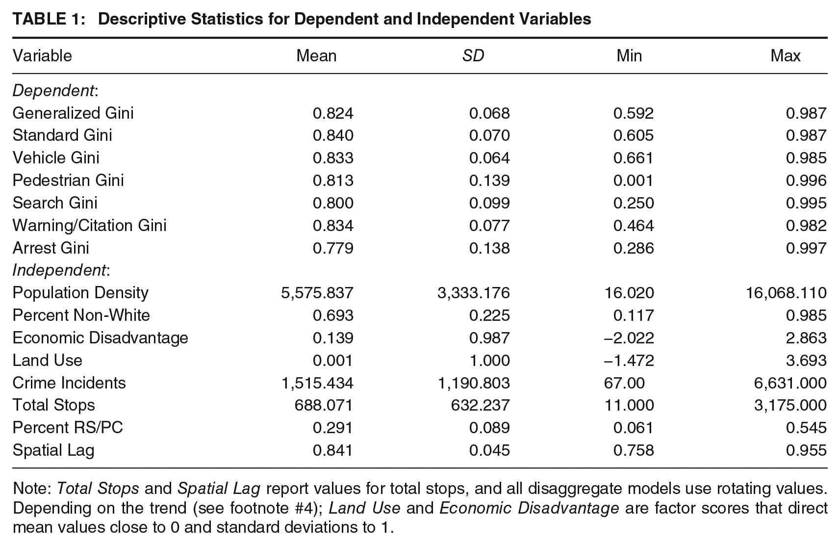
Note: Total Stops and Spatial Lag report values for total stops, and all disaggregate models use rotating values. Depending on the trend (see footnote #4); Land Use and Economic Disadvantage are factor scores that direct mean values close to 0 and standard deviations to 1.

Results

Spatial Distribution of Stops

We found there was substantial concentration of police stops between micro-places in Oakland. Around 3% of the street units accounted for 50% of the total stops during our observation period. All 77,752 of the police-civilian stops were distributed across only 34.7% of the total street units. The city-wide Gini coefficient was 0.878 which reinforces that there is much distributional concentration of these contacts at micro-places within Oakland. The generalized Gini coefficients for each of the 113 census tracts in Oakland were normally distributed. The mean coefficient is 0.824, which is slightly less than the city-wide value with a standard deviation of 0.068. The maximum value is 0.987, which suggests a remarkable concentration of stops within this census tract, and the minimum value is 0.592, which is an observable outlier. This value indicates a comparatively more diffused spatial distribution of stops within this census tract. Based on the distribution, the middle 50% of observations ranged between 0.783 and 0.872.

Figure 1 displays localized kernel density maps of the census tracts which had low, average, and high values of Gini coefficients. These maps allow for the twofold interpretation of both the extent of the micro-places that experienced stops and provide a sense of the volume of stops found at these locations. “Tract A” contains the second lowest value in the distribution (G’ = 0.604) and presents a neighborhood where there is a noticeable diffusion of stops across micro-places. There are only a few hot spots of stops, with most stops diffused across various other locations throughout the neighborhood. Thus, people living or using the space within this neighborhood face increased spatial exposure to police contacts because the police are likely to stop people across more places. “Tract B” displays a more average neighborhood (G’ = 0.827) in Oakland with a larger Gini coefficient therefore more concentration of stops. This coefficient is manifested as a similar number of hot spots but a seemingly smaller number of other locations with stops across this larger neighborhood. Finally, “Tract C” displays the tract with the highest concentration of stops (G’ = 0.987). This neighborhood had one street unit that contained almost all the stops over the entire observation period. While there is noteworthy variation, these descriptive statistics suggest the predominant condition across all locations is concentration of stops since most Gini coefficients are large values (see Online Supplemental Material).

Figure 1:

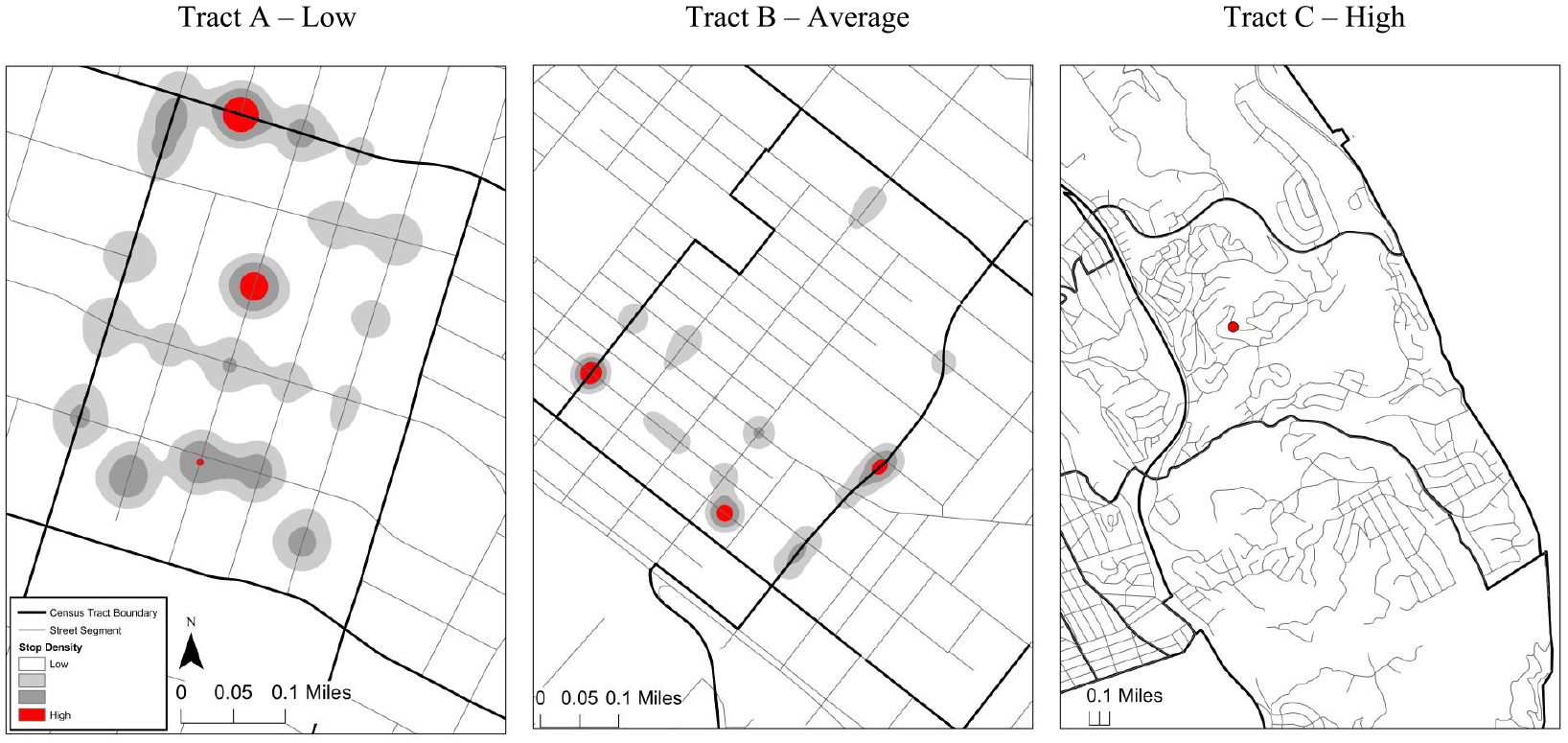
The Spatial Distribution of Total Stops Across Three Census Tracts using Localized Kernel Densities

Explanatory Models

Table 2 displays the results of four models, which contrast the use of different strategies for calculating Gini coefficients. Models 1 and 2 use the standard calculation of Gini coefficients as the dependent variable. Model 1 observes three of four structural variables that provide a statistically significant explanation for variation in the distribution of stops between neighborhoods. Model 2 includes all four control variables, with only one displaying statistical significance. The results from Model 2 suggest the higher percentage of non-white residents in a census tract is associated with a lower, statistically significant (p = .004) Gini coefficient for police stops or a more diffused pattern of stops. These results also suggest the tracts Gini coefficients are positively associated with their surrounding neighborhoods’ values.

Table 2:

Results of Linear Regression Models using Two Versions of Gini Coefficients for Total Stops

Ind. Variables	Standard Gini				Generalized Gini
	Model 1		Model 2		Model 3		Model 4
	Beta (SE)	Std. beta	Beta (SE)	Std. beta	Beta (SE)	Std. beta	Beta (SE)	Std. beta
Pop. Density	0.01*** (0.01)	−0.25	0.01* (0.01)	−0.17	0.00(0.01)	−0.04	0.01(0.01)	−0.03
Pct. Non-White	−0.11** (0.04)	−0.36	−0.13** (0.04)	−0.41	−0.12*(0.05)	−0.38	−0.17**(0.06)	−0.57
Econ. Disadv.	−0.02+ (0.01)	−0.24	0.01 (0.01)	−0.07	0.00(0.01)	0.06	0.01(0.01)	0.17
Land Use	−0.01** (0.01)	−0.20	−0.01 (0.01)	−0.17	−0.01(0.01)	−0.14	−0.02*(0.01)	−0.32
Crime Incidents	-	-	0.01 (0.01)	−0.04	-	-	0.01(0.01)	0.23
Total Stops	-	-	0.01+ (0.01)	0.20	-	-	0.01(0.01)	0.03
Pct. RS/PC	-	-	0.09 (0.05)	0.11	-	-	−0.06(0.07)	−0.08
Spatial Lag	-	-	0.50** (0.18)	0.32	-	-	−0.04(0.22)	−0.02
R ²	0.53		0.58		0.14		0.18

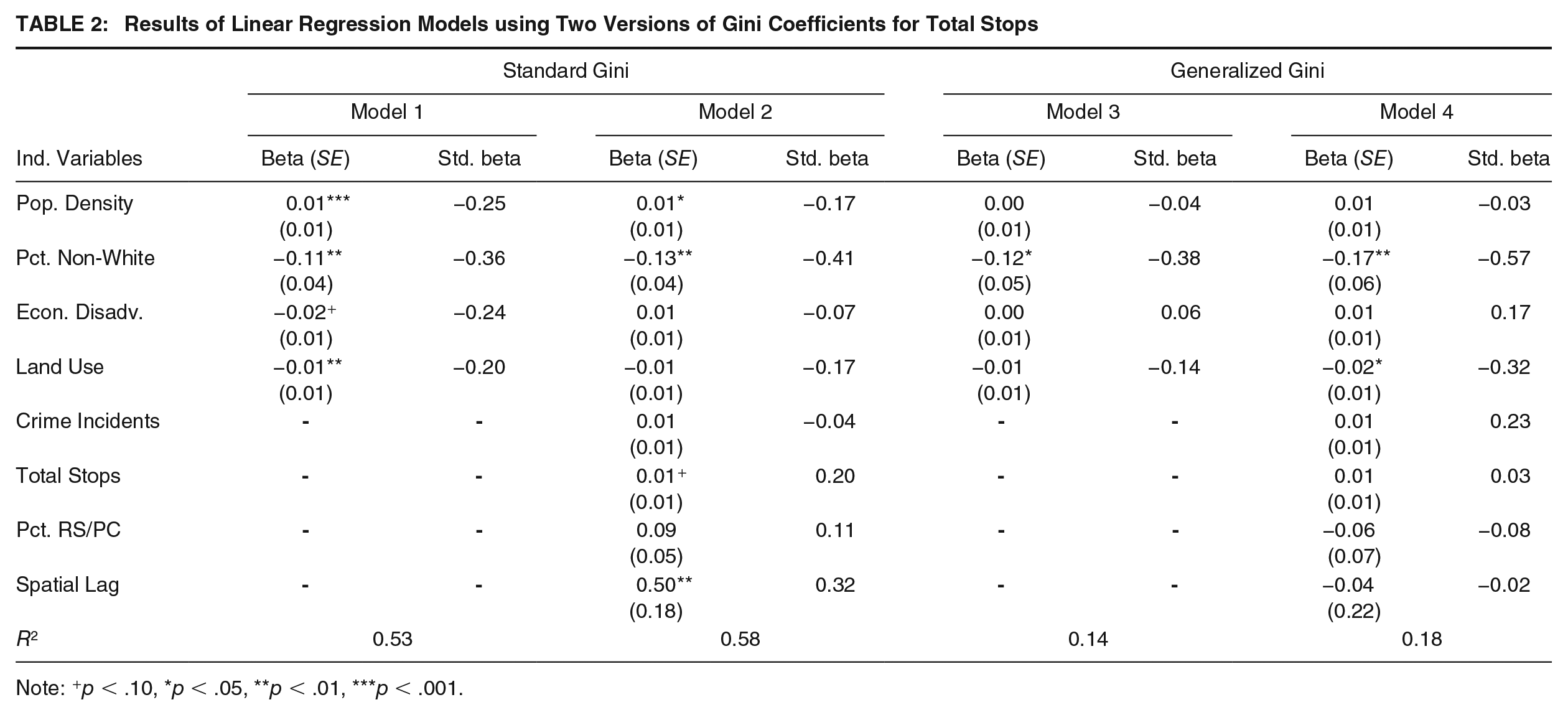
Note: +p < .10, *p < .05, **p < .01, ***p < .001.

Models 3 and 4 use the generalized calculation of Gini coefficients as the dependent variable to adjust for the census tracts that have more street units than police stops. Model 3 displays notable differences compared to Model 1. The R² value is drastically reduced, and only the percent of non-white residents remains statistically significant. Model 4 retains the statistical significance of the percentage non-white variable, and the land use variable becomes statistically significant. Models 3 and 4 are much closer to the R² threshold of 0.125 established by the power analysis. The effect of race/ethnicity of neighborhood residents remains statistically significant across all models and accounting for control variables. In general, these models indicate that the calculation method of the coefficient does influence the effects found for both structural and control variables. The adjustment across 13 census tracts had a noticeable impact with only a small number of observations (i.e., 11.5% of total) and the downward adjustment toward diffusion of contacts.

Table 3 presents the results from five models with disaggregated categories of stops as the dependent variables. There is modest variation in the R² values across each model which indicates that different explanations were more salient to predict certain categories. Only Model 4 was close to our R² threshold. This suggests there could be different types of mechanisms or nuances necessary to unpack explanations for these different patterns of categories of stops. The percent non-white variable had the most consistent results across each of the models. This variable was statistically significant across all five models and remained negatively associated with Gini coefficients for stops. In other words, the police are contacting people in more places as there are more people of color living in neighborhoods. This effect is robust after inclusion of control variables and across different categories of stops. The economic disadvantage variable was statistically significant across three of the models. For example, this finding indicates census tracts with greater economic disadvantage are associated with increases in the concentration of pedestrian stops (Model 2), stops that led to a search (Model 3), and stops that led to an arrest (Model 5). These categories where economic disadvantage had a significant effect are associated with stops where a pedestrian is more visible (i.e., compared to vehicle stops) and stops with search and arrest outcomes, which are more severe outcomes.

Table 3:

Results of Linear Regression Models on Gini Coefficients for Disaggregate Stop Categories

Ind. Variables	Vehicle		Pedestrian		Search		Warning/citation		Arrest
	Model 1		Model 2		Model 3		Model 4		Model 5
	Beta (SE)	Std. beta	Beta (SE)	Std. beta	Beta (SE)	Std. beta	Beta (SE)	Std. beta	Beta (SE)	Std. beta
Pop. Density	0.01 (0.01)	−0.04	0.01(0.01)	0.13	0.01(0.01)	0.06	0.01(0.01)	0.01	0.01+(0.01)	0.16
Pct. Non-White	−0.13*(0.05)	−0.46	−0.24*(0.11)	−0.38	−0.19*(0.08)	−0.44	−0.15*(0.07)	−0.42	−0.24*(0.11)	−0.39
Econ. Disadv.	0.01 (0.01)	0.06	0.07**(0.02)	0.49	0.05**(0.02)	0.51	0.02(0.02)	0.20	0.09**(0.02)	0.63
Land Use	−0.02*(0.01)	−0.33	−0.02(0.02)	−0.16	−0.02(0.01)	−0.21	−0.03*(0.01)	−0.36	−0.02(0.02)	−0.13
Crime Incidents	0.01 (0.01)	0.25	0.01(0.01)	0.08	0.01+(0.01)	0.28	0.01+(0.01)	0.30	0.01(0.01)	0.22
Total Stops^	0.01 (0.01)	−0.06	0.01+(0.01)	0.27	0.01(0.01)	−0.02	0.01(0.01)	0.01	0.01(0.01)	0.20
Pct. RS/PC	−0.12+ (0.07)	−0.16	0.04(0.13)	0.03	0.02(0.10)	0.01	−0.22*(0.08)	−0.25	0.10(0.13)	0.06
Spatial Lag^	−0.03 (0.22)	−0.01	0.30+(0.15)	0.20	0.55**(0.18)	0.31	0.06(0.20)	0.03	−0.02(0.18)	−0.01
R ²	0.21		0.30		0.22		0.14		0.34

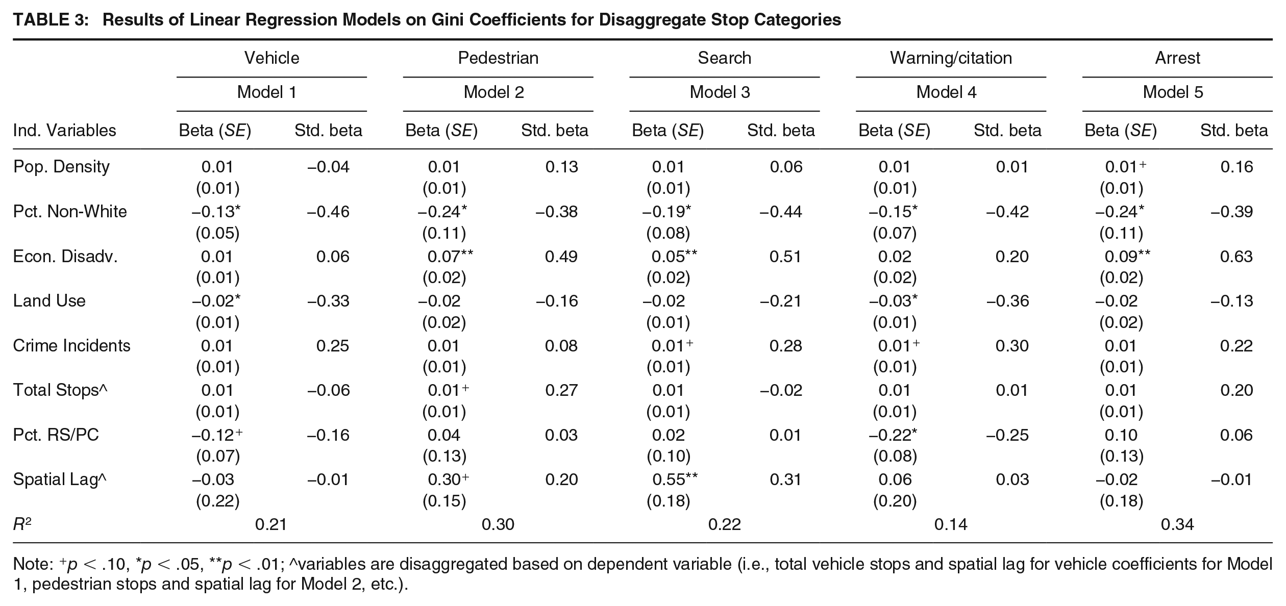
Note: +p < .10, *p < .05, **p < .01; ^variables are disaggregated based on dependent variable (i.e., total vehicle stops and spatial lag for vehicle coefficients for Model 1, pedestrian stops and spatial lag for Model 2, etc.).

The significance of economic disadvantage is noteworthy because, per Table 3, the variable was not significant for the generalized coefficient, and the standard Gini models with the direction of the effect were different. The effect of race/ethnicity and economic disadvantage further reinforces there is a connection between where the police stop people and the sociodemographic characteristics of these neighborhoods. Increases in the percent of non-white residents are associated with decreases in the Gini coefficient for stops while increases in the percent of residents living under economic disadvantage are associated with increases in Gini coefficient of stops. The directional divergence of these two effects presents an interesting finding since we anticipated both would operate in the same direction (see Online Supplemental Material). The only other variable that reached statistical significance across two or more of these disaggregate stop categories was land use. Both the spatial lag and percent RS/PC variables achieved statistical significance only one time. The total number of incidents was not a robust predictor of Gini coefficients for police stops. These findings suggest the amount of crime in a neighborhood did not impact where the police stopped civilians.

Between the seven models reported in Tables 2 and 3, the total number of stops in a neighborhood was not a statistically significant predictor of differences in the Gini coefficient of stops. This reinforces the frequency of stops and where they occur are not necessarily connected. This highlights the importance of observing the Gini coefficient as a new dimension. We conducted several supplemental analyses to determine the sensitivity of the race/ethnicity findings that are featured in the Online Supplemental Material. In general, these analyses confirmed our results by demonstrating this variable provided the most consistent explanation for variation in Gini coefficients for police contacts.

Discussion

Main Findings

Overall, we observed there is moderate variability in the spatial exposure of micro-places to police contacts between neighborhoods. Most neighborhoods experienced concentration of stops at micro-places, but there was noteworthy variability in the distribution of these measures between micro-places. The overall degree of concentration across all neighborhoods was striking. Based on the distribution of Gini coefficients, the variability just captures relatively modest changes in the degree to which police contacts are concentrated. We found our parsimonious models were generally helpful in explaining variation in the distribution of police contacts at micro-places between neighborhoods. The main finding from the explanatory analyses was the only consistent predictor of Gini coefficients for police stops across models was the race/ethnicity of neighborhood residents. Regardless of the nature of the stop (i.e., vehicle, pedestrian, or both) or outcome of the stop examined (i.e., warning/citation, search, or arrest), the racial/ethnic characteristics of community residents were the most consistent predictor of variation in the distribution of Gini coefficients of police contacts between neighborhoods. In other words, as neighborhoods had more non-white residents, the general spatial exposure of these communities to police contacts increased. This explanation extends beyond the scope of the routine police work hypothesis and provides some limited support for the social characteristics hypothesis. We urge much caution with the interpretation of this finding. There is no definitive interpretation we recommend, and instead, several possibilities which we believe warrant further consideration.

Theoretical and Policy Implications

The effect of racial/ethnic composition of neighborhoods may just represent other ecological characteristics that influence spatial patterns of police contracts, which we did not measure in our models. Research has shown that certain facilities (i.e., check cashing) and site features (i.e., abandoned buildings) are more likely to be nested within disadvantaged areas, which influences the overall crime risk of these areas (Eck, 2018). These places then may receive a certain label or stigmatization from officers by which they gravitate to these neighborhoods and contact civilians not because of the racial/ethnic composition but because of these other ecological characteristics. In addition, increased spatial exposure to police contacts is not inherently problematic. We discussed in the literature review how several types of police contacts are associated with positive effects for civilians. Our analyses do not explain the dynamics of the interactions that occur between police and these community members during these stops. The police contacting people in more places just demonstrates a different ecological behavioral pattern of police practices, not one that is necessarily positive or negative. On the other hand, the research connecting police contacts and race/ethnicity is relatively straightforward (Weitzer & Tuch, 2006), and the lack of any other explanation for these divergent patterns of police practices could be assumed as concerning by default. The racial/ethnic gap in approval of policing practices discussed in our literature review, at the very least, suggests this increased spatial exposure would likely be perceived with much skepticism by these diverse communities. In general, any association between divergent police behaviors and social characteristics such as race/ethnicity is worth further investigation.

Our findings could be interpreted to provide some support for critical perspectives on race and policing, which argue police behavior is influenced by social characteristics of individuals. Specifically, the finding suggests the police may decide to stop people in more locations and cast a larger “net” over certain neighborhoods based on race/ethnicity. Our models do account for other important control variables such as the level of crime, total number of stops, and the underlying justification for the stop, which are some of the major confounding variables of this effect. We believe using the concept of over-policing is a reasonable approach to help interpret our results. Research suggests some places experience over-policing or increased susceptibility to police presence based on the racial/ethnic composition of communities (Crowther, 2013). Our findings could offer empirical support to this perspective and suggest that over-policing is manifested as the diffusion of more contacts across places.

While research on over-policing is rightfully critiqued for not establishing a baseline expectation for levels of policing (see Neil & Winship, 2019), our regression analyses do provide this comparison based on the distribution of these contacts across all neighborhoods in Oakland. Therefore, the more racially/ethnically diverse neighborhoods are in Oakland, the more exposure these places get to police contacts relative to the other neighborhoods in the city. While there is still much definitional debate on the issues of over- and under-policing, this study could provide a contribution to conceptualizing this idea through an entirely spatial perspective. Again, we offer much caution to this interpretation, and we understand not all readers may agree with this connection, but we nonetheless offer this interpretation to inform this broader debate. Proponents of the over-policing perspective could further argue both increased frequency and spatial exposure are justifications to show why some places receive unequal access to the police based on race/ethnicity. In other words, increased spatial exposure could be considered a “force multiplier” for this argument by saying some places get more contacts and more places receive contacts relative to baseline expectations. Thus, we present an additive, second-order dimension to consider levels of police presence. Regardless of the specific interpretation you prefer for our findings, we believe our results are an interesting empirical contribution to the literature on police behavior and practices, which warrants further investigation. Understanding why these patterns diverge between places is even more challenging. Why does police behavior change across places, and how does race influence decision-making?

This question leads to an examination of policy focused on two key areas: officer decision-making and the organizational psychology of police departments. First, some police officers may have implicit biases which influence their decision-making. Police departments have increasingly embraced this idea, which has firm roots in psychological research and have provided new training to officers on this topic (see Fridell & Lim, 2016). In contrast, some may argue that police officers repeatedly engage in unconstitutional and discriminatory policing behaviors. Some scholars contend that certain police officers may have explicit racial biases and associate non-white civilians as more criminal, resulting in these individuals being stopped across more places throughout neighborhoods (see Hall et al., 2016).

Second, we must consider the organizational psychology of police departments that may influence the behavior of officers regarding the relationship between race/ethnicity and contacts. These systemic explanations are more persuasive interpretations of our findings because this effect is collectively observed behavior across a large police department. While the actions of a small handful of officers could disproportionately influence police agencies’ statistics (Chalfin & Kaplan, 2021), the broader patterns are a manifestation of behavior across large numbers of officers within a department. For example, OPD has around 700 sworn officers. Thus, the lack of monitoring and control of these potentially biased behaviors is ultimately the responsibility of the police department. It could be that police agencies may not be providing adequate training, have weak internal investigations, and/or establish a culture that does not hold “bad apples” accountable. These organizational issues are at the center of the US Department of Justice patterns and practice investigations, which use consent decrees to enact broad reforms at departments. Our findings could just capture the underlying patterns of bias that led to Oakland receiving this monitoring and are not generalizable to other jurisdictions. Future research should consider exploring this relationship across different cities.

Conclusion

There were a few other limitations to our study which could inform future research. We conducted a cross-sectional analysis which provides challenges to making causal inference because of temporal ordering. Our independent variables also provided conceptual challenges since our neighborhood effects variables such as crime incidents and police stops are often highly intercorrelated in a feedback loop. OPD could not provide us with calls for service data for our observation period which may have provided a different interpretation instead of the crime incident report variable we used as a control measure. Despite the empirical reality of where the police are stopping people, the perceptual reality of where the police could have a presence or individual’s accumulated vicarious experiences are still powerful considerations. These perceptions influence individuals’ cognitive landscapes of how the police interact with places and where they think the police operate (i.e., perceptual vs. actual exposure). Nevertheless, this study contributes an innovative analysis and presents new directions for future research to explore which could mitigate these limitations to improve understanding of the ecology of police-civilian contacts.

In conclusion, we will address this study’s titular question: where do cops stop? The most consistent predictor of this uneven distribution of contacts was the racial/ethnic characteristics of neighborhoods. Future research should build upon this approach to further explain spatial patterns of police-civilian contacts. Our research expands upon scholarship across disciplines such as public health, which have routinely examined exposures to specific environments on later health outcomes (see Knowlden et al., 2015). The use of this measure could inform public health research that focuses on reciprocal determinism, exposure to unhealthy environments, and adverse social determinants of health that influence the future health of Americans. During a time when police resources are limited, our analyses provide a framework for how police agencies can improve upon their data analytics by incorporating spatial analyses to address issues associated with police–community relationships.

Supplemental Material

sj-docx-1-cjb-10.1177_00938548241249700 – Supplemental material for Where Do Cops Stop? A New Dimension to Explore Spatial Patterns of Police Contacts

Supplemental material, sj-docx-1-cjb-10.1177_00938548241249700 for Where Do Cops Stop? A New Dimension to Explore Spatial Patterns of Police Contacts by Cory Schnell and Hunter Boehme in Criminal Justice and Behavior

Footnotes

Author’s Note:

We would like to thank Leigh Grossman and the Oakland Police Department for helping us access and learn more about the police contact data.

ORCID iD

Cory Schnell

Supplemental Material

Supplemental Material is available in the online version of this article at

Notes

Cory Schnell is an Assistant Professor at the University of South Carolina in the Department of Criminology and Criminal Justice. His research interests include place-based criminology, policing, and violence.

Hunter Boehme is an Assistant Professor at the University of South Carolina in the Department of Criminology and Criminal Justice. His research interests include policing, place-based criminology, and hate crimes.

References

Adams

R. E.

Rohe

W. M.

Arcury

T. A.

(2005). Awareness of community-oriented policing and neighborhood perceptions in five small to midsize cities. Journal of Criminal Justice, 33(1), 43–54. https://doi.org/10.1016/j.jcrimjus.2004.10.008

Bernasco

Elffers

(2010). Statistical analysis of spatial crime data. In Piquero

A. R.

Weisburd

(Eds.), Handbook of quantitative criminology (pp. 699–724). Springer. https://doi.org/10.1007/978-0-387-77650-7_33

Bernasco

Steenbeek

(2017). More places than crimes: Implications for evaluating the law of crime concentration at place. Journal of Quantitative Criminology, 33(3), 451–467. https://doi.org/10.1007/s10940-016-9324-7

Boehme

H. M.

Cann

Isom

D. A.

(2020). Citizens’ perceptions of over-and under-policing: A look at race, ethnicity, and community characteristics. Crime & Delinquency, 68(1), 123–154. https://doi.org/10.1177/0011128720974309

Bolger

M. A.

Lytle

D. J.

Bolger

P. C.

(2021). What matters in citizen satisfaction with police: A meta-analysis. Journal of Criminal Justice, 72(1), Article 101760. https://doi.org/10.1016/j.jcrimjus.-2020.101760

Braga

A. A.

Brunson

R. K.

Drakulich

K. M.

(2019). Race, place, and effective policing. Annual Review of Sociology, 45(1), 535–555. https://doi.org/10.1146/annurev-soc-073018-022541

Braga

A. A.

Papachristos

A. V.

Hureau

D. M.

(2010). The concentration and stability of gun violence at micro places in Boston, 1980–2008. Journal of Quantitative Criminology, 26(1), 33–53. https://doi.org/10.1007/s10940-009-9082-x

Brantingham

P. J.

Brantingham

P. L.

(1991). Environmental criminology. Sage.

Brunson

R. K.

(2007). Police don't like black people: African-American young men's accumulated police experiences. Criminology & Public Policy, 6(1), 71–101. https://doi.org/10.1111/j.1745-9133.2007.00423.x

10.

Carr

P. J.

Napolitano

Keating

(2007). We never call the cops and here is why: A qualitative examination of legal cynicism in three Philadelphia neighborhoods. Criminology & Public Policy, 45(2), 445–480. https://doi.org/10.1111/j.1745-9125.2007.00084.x

11.

Carroll

Gonzalez

M. L.

(2014). Out of place: Racial stereotypes and the ecology of frisks and searches following traffic stops. Journal of Research in Crime and Delinquency, 51(5), 559–584. https://doi.org/10.1177/0022427814523788

12.

Chalfin

Kaplan

(2021). How many complaints against police officers can be abate by incapacitating a few bad apples? Criminology & Public Policy, 20(2), 351–370. https://doi.org/10.1111/1745-9133.12542

13.

City of Oakland. (2019). Oakland police department—Negotiated settlement agreement (NSA). https://www.oaklandca.gov/documents/oakland-police-department-negotiated-settlement-agreement-nsa

14.

Crowther

(2013). Over-policing and under-policing social exclusion. In Burke

R. H.

(Eds.), Hard cop, soft cop (pp. 63–77). Willan. https://doi.org/10.4324/9781843924531

15.

Eck

J. E.

(2018). Race, place management, and crime. In Unnever

J. D.

Gabbidon

S. L.

Chouhy

(Eds.), Building a black criminology, volume 24: Race, theory, and crime (pp. 1–36). Routledge.

16.

Foster

Jones

M. S.

Pierce

(2022). Race and ethnicity differences in police contact and perceptions of and attitudes toward the police among youth. Criminal Justice and Behavior, 49(5), 660–680. https://doi.org/10.1177/00938548221078296

17.

Fridell

Lim

(2016). Assessing the racial aspects of police force using the implicit and counter-bias perspectives. Journal of Criminal Justice, 44(3), 36–48. https://doi.org/10.1016/j.jcrimjus.2015.12.001

18.

Gill

Weisburd

Telep

C. W.

Vitter

Bennett

(2014). Community-oriented policing to reduce crime, disorder and fear and increase satisfaction and legitimacy among citizens: A systematic review. Journal of Experimental Criminology, 10(4), 399–428. https://doi.org/10.1007/s11292-014-9210-y

19.

Hall

A. V.

Hall

E. V.

Perry

J. L.

(2016). Black and blue: Exploring racial bias and law enforcement in the killings of unarmed black male civilians. American Psychologist, 71(3), 175–186. https://doi.org/10.1037/a0040109

20.

Huff

(2021). Understanding police decisions to arrest: The impact of situational, officer, and neighborhood characteristics on police discretion. Journal of Criminal Justice, 75(7), Article 101829. https://doi.org/10.1016/j.jcrimjus.2021.101829

21.

Kelling

G. L.

Pate

Dieckman

Brown

C. E.

(1974). Kansas City preventative patrol experiment: A summary report. Police Foundation.

22.

Klinger

D. A.

(1997). Negotiating order in patrol work: An ecological theory of police response to deviance. Criminology; An Interdisciplinary Journal, 35(2), 277–306. https://doi.org/10.1111/j.1745-9125.1997.tb00877.x

23.

Knowlden

A. P.

Sharma

Cottrell

R. R.

Wilson

B. R.

Johnson

M. L.

(2015). Impact evaluation of enabling mothers to prevent pediatric obesity through web-based education and reciprocal determinism (EMPOWER) randomized control trial. Health Education & Behavior, 42(2), 171–184. https://doi.org/10.1177/1090198114547816

24.

Neil

Winship

(2019). Methodological challenges and opportunities in testing for racial discrimination in policing. Annual Review of Criminology, 2, 73–98. https://doi.org/10.1146/annurev-criminol-011518-024731

25.

Nouri

(2021). Police use of force at street segments: Do street-level characteristics matter? Journal of Criminal Justice, 77(11), Article 101862. https://doi.org/10.1016/j.jcrimjus.2021.101862

26.

O’Brien

D. T.

Ciomek

Tucker

(2021). How and why is crime more concentrated in some neighborhoods than others? A new dimension to community crime. Journal of Quantitative Criminology, 38, 1–27. https://doi.org/10.1007/s10940-021-09495-9

27.

Papachristos

A. V.

Braga

A. A.

Piza

Grossman

L. S.

(2015). The company you keep? The spillover effects of gang membership on individual gunshot victimization in a co-offending network. Criminology, 53(4), 624–649. https://doi.org/10.1111/1745-9125.12091

28.

Ratcliffe

(2010). Crime mapping: Spatial and temporal challenges. In Piquero

A. R.

Weisburd

(Eds.), Crime mapping: Spatial and temporal challenges (pp. 5–24). Springer. https://doi.org/10.1007/978-0-387-77650-7_2

29.

Rios

V. M.

(2011). Punished: Policing the lives of Black and Latino boys. NYU Press.

30.

Sampson

R. J.

Morenoff

J. D.

Gannon-Rowley

(2002). Assessing neighborhood effects: Social processes and new directions in research. Annual Review of Sociology, 28, 443–478. https://doi.org/10.1146/annurev.soc.28.110601.141114

31.

Schnell

Braga

A. A.

Piza

E. L.

(2017). The influence of community areas, neighborhood clusters, and street segments on the spatial variability of violent crime in Chicago. Journal of Quantitative Criminology, 33(3), 469–496. https://doi.org/10.1007/s10940-016-9313-x

32.

Skogan

W. G.

(2005). Citizen satisfaction with police encounters. Police Quarterly, 8(3), 298–321. https://doi.org/10.1177/1098611104271086

33.

Slocum

L. A.

Wiley

S. A.

(2018). Experience of the expected? Race and ethnicity differences in the effects of police contact on youth. Criminology, 56(2), 402–432. https://doi.org/10.1111/1745-9125.12174

34.

Steenbeek

Bernasco

(2018). Lorenzgini: Generalized Gini for sparse data situations. R Package. https://github.com/wsteenbeek/lorenzgini

35.

Tapp

S. N.

Davis

(2022). Contacts between police and the public, 2020. Bureau of Justice Statistics.

36.

Terrill

Reisig

M. D.

(2003). Neighborhood context and police use of force. Journal of Research in Crime and Delinquency, 40(3), 291–321. https://doi.org/10.1177/002242-7803253800

37.

Tyler

T. R.

(2004). Enhancing police legitimacy. The Annals of the American Academy of Political and Social Science, 593, 84–99. https://doi.org/10.1177/0002716203262627

38.

United States Census Bureau. (2022). QuickFacts: Oakland, California. United States Census Bureau. https://www.census.gov/quickfacts/fact/table/US/PST045223

39.

Weisburd

Braga

A. A.

(2019). Police innovation: Contrasting perspectives (2nd ed.). Cambridge University Press.

40.

Weitzer

Tuch

S. A.

(2006). Race and policing in America: Conflict and reform. Cambridge University Press.

Supplementary Material

Please find the following supplemental material available below.

For Open Access articles published under a Creative Commons License, all supplemental material carries the same license as the article it is associated with.

For non-Open Access articles published, all supplemental material carries a non-exclusive license, and permission requests for re-use of supplemental material or any part of supplemental material shall be sent directly to the copyright owner as specified in the copyright notice associated with the article.

0.00 MB

0.07 MB