Marginal-Preserving Imputation of Three-Way Array Data in Nested Structures,with Application to Small Areal Units

Abstract

Geospatial population data are typically organized into nested hierarchies of areal units, in which each unit is a union of units at the next lower level. There is increasing interest in analyses at fine geographic detail, but these lowest rungs of the areal unit hierarchy are often incompletely tabulated because of cost, privacy, or other considerations. Here, the authors introduce a novel algorithm to impute crosstabs of up to three dimensions (e.g., race, ethnicity, and gender) from marginal data combined with data at higher levels of aggregation. This method exactly preserves the observed fine-grained marginals, while approximating higher-order correlations observed in more complete higher level data. The authors show how this approach can be used with U.S. census data via a case study involving differences in exposure to crime across demographic groups, showing that the imputation process introduces very little error into downstream analysis, while depicting social process at the more fine-grained level.

Many data sources, including the U.S. census and organizations using Google’s S2 projection system, ¹ provide geospatial population data organized into a nested hierarchy of areal units. In such hierarchical structures, each areal unit at a given level can be expressed as the union of a set of units at the level below, in turn being part of a single parent; each level is hence a spatial partition of the region of interest (see Figure 1). Many sociological questions involve the cross-tabulation of population properties within such units with other quantities (e.g., environmental, ecological, political, economic, or other variables that vary across regions). With the advent of increasingly well-developed spatial data sets (Facebook Connectivity Lab, Center for International Earth Science Information Network, and Columbia University 2016; Rose et al. 2021), performing such analyses at increasingly fine geographic resolution is of substantial interest (Thomas et al. 2020).

Figure 1.

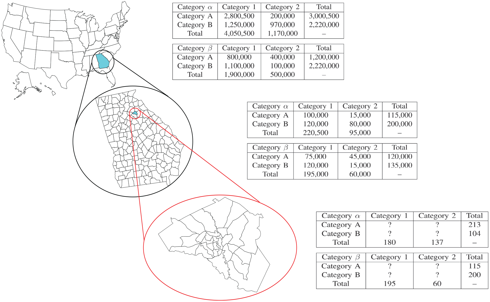
An example of a hierarchical data structure on areal units, using the U.S. census areal unit hierarchy.

In practice, however, such fine-grained analyses can still encounter problems of data availability. For instance, although detailed census data are publicly released at higher levels of the census geography (e.g., counties), incomplete data are released at smaller geographic scales (e.g., blocks and block groups). This issue is not unique to the U.S. census: releasing fully detailed information at fine scale poses challenges of acquisition cost (there are vastly more small areal units than large ones), availability (key variables may not be obtained at all scales), distribution and maintenance costs, and privacy considerations. Where information for smaller units is available, it is often available only marginally (i.e., summed across all values of a covariate), without the cross-tabulation needed to study many demographic processes. For instance, we may know how many individuals reside in a given unit by race, by ethnicity, and by gender, but we may not know how many White Hispanic women reside there. Raising our level of analysis to the smallest unit with complete tabulation may resolve this difficulty, but at the cost of “blurring” spatial heterogeneity. This can cause problems for analysis, particularly when studying phenomena that occur on small scales (e.g., neighborhood interactions, exposure to crime or other events, or immediate access to local amenities).

Although there is no perfect substitute for complete data, the presence of incompletely tabulated data suggests the viability of imputation strategies: even one-way marginals can be powerfully constraining, and two-way marginals even more so. When marginals can be combined with information on correlations from higher-order units with complete data, it may be possible to accurately estimate the local tabulation in a way that preserves all known quantities. This preserves spatial heterogeneity and permits fine-grained analysis, while also making use of more complete information where available. Surprisingly, this approach to the multiway areal unit imputation problem appears to have been overlooked in prior literature, although we draw on a number of related developments in our work (as described later).

In this article, we introduce a method for imputing cross-tabulated count data organized into a nested system of hierarchical bins, which is highly parallelizable and hence applicable to large systems (including the U.S. census). We focus on the case in which data are cross-tabulated with up to three different discrete features, each of which may take on a number of values (i.e., a three-way crosstab); our approach combines lower-order information on marginals from the focal bin with more complete, higher-order marginals from the bin’s parent to impute the full multiway array. We can verifiably preserve all available information on the focal bin (assuming such data are consistent), while approximating higher-order information to the extent possible given low-order constraints. Our technique also allows either point estimation, or simulation of draws from the conditional maximum entropy distribution of the target array given the observed data constraints, supporting use cases such as multiple imputation, which can offer consistent uncertainty measures (Rubin 1996). As an illustration of the method, we apply our approach to imputation of small areal unit data using the 2010 U.S. decennial census, demonstrating how it enables fine-grained ecological analysis (here, of differences in exposure to crime) despite data constraints.

Prior Work

As noted, the specific problem of marginal-preserving multiway count-data imputation from combined marginal and hierarchical information seems not to have been addressed in prior work. However, a number of related problems have been studied, solutions to which inform our own approach. By way of background, we thus begin by reviewing related results on small areal unit estimation and imputation for three-way crosstabs, both of which set the stage for our work.

Small Areal Unit Estimation

In its more general context, the problem of inferring characteristics of (usually small) geographic regions is known as the small area estimation (SAE) problem. This challenge arises in many different fields, and work on SAE has bridged a number of disciplines, including but not limited to sociology, demography (Morrison 1971), and statistics (Bunea and Besag 2000; Graham, Young, and Penny 2009). Small areal unit estimation often deals with estimation of population demographics, but some work goes beyond this to examine covariates such as poverty or disease (Molina and Rao 2010; Pfeffermann 2013). These techniques are also applicable to examination of crime exposure in a population, as we explore here. There are numerous strategies for this problem, ranging from simpler strategies such as uniform imputation (completely uninformed at the small geographic unit) or spatial smoothing techniques such as kriging that attempt to flexibly exploit spatial autocorrelation across units (Bennett, Haining, and Griffith 1984; Mooney et al. 2020), to more informed model-based approaches (Cohen and Zhang 1988; Steinberg 1979). Related to this work, some researchers have specifically examined maintaining structural constraints and the use of model assisted approaches (Espuny-Pujol, Morrissey, and Williamson 2018; Luna et al. 2015; Moretti and Whitworth 2020).

In the field of criminology, the interest in estimating models in which crime is an outcome measure in increasingly small geographic units has resulted in a need for SAE. Whereas some scholars have simply used a uniform imputation strategy to assign data from a larger geographic unit to a smaller unit, another strategy uses synthetic estimation for ecological inference (Boessen and Hipp 2015). This strategy requires the assumption that the relationships between variables in the larger geographic units are the same as the relationships within the smaller geographic subunits.

Surprisingly few studies in criminology or sociology have explored the exposure to crime of different demographic groups. Arguably, this state of affairs is due to the difficulty of obtaining crime data at a more granular scale. For example, Alba, Logan, and Bellair (1994) measured the context of small suburban communities (defined as population less than 10,000) in assessing exposure to crime. Another study in Cleveland aggregated census tracts to “neighborhoods,” and thus an even larger geographic unit (Logan and Stults 1999). Yet another study measured the context as police precincts in New York City, which are larger, given that at the time of the study, there were 75 precincts in a city with more than 7 million residents (McNulty 1999). The challenge is that such units may be too large to capture the environment of a specific person, or group of people. This issue arises in the context of other social exposures, as well; for instance, Thomas et al. (2020, 2022) provide evidence that both infection hazards and social exposure to others’ morbidity and mortality in the early COVID-19 pandemic was affected by local variation in network structure influenced by housing and demographic factors at or below the block scale. Such differences in exposure may affect not only immediate health outcomes, but also responsiveness to public health interventions, with consequences for both policy effectiveness and health disparities.

The SAE problem is computationally challenging, both because it often involves discrete optimization (e.g., for population counts) and because SAE solutions are often intended to be used at scale; for example, given that the United States has more than 8 million census blocks, and there are more than 1.6 billion level 14 S2 cells worldwide (each about 500 m across), efficiency can be a significant concern. As such, work on this problem has spurred a range of computational advances, from algorithms to actually perform estimation (Graham et al. 2009; Vermunt et al. 2008) to the evaluation of produced results (Pfeffermann and Correa 2012). Many of the more statistically principled algorithms derive from the literature on hierarchical Bayesian modeling, which provides numerous conceptual and statistical tools for flexible estimation and incomplete pooling of information across units (King, Rosen, and Tanner 1999). Although these frameworks often require significant computational resources, as the Markov chain Monte Carlo (MCMC) algorithms required for fitting and simulating draws from such models (Rosen et al. 2001) are computationally intensive, the algorithms enable estimations of more complex problems where the joint probability functions are not in closed form.

In this context, our work contributes to the SAE literature by implementing an algorithm for small areal unit estimation that can produce imputed cross-classification data for areal units that satisfy a complex constraint structure (guaranteeing that imputations exactly preserve one- and two-way marginal totals, and are integer-valued), while also including information from higher-order units. Our technique draws on the statistical strengths of the SAE literature by leveraging a hierarchical model, extending the work of Bunea and Besag (2000) by including additional information about the composition of larger areal units in the imputation process.

Imputation for Cross-Tabulated Count Data

Apart from the SAE problem, our work is also related to the general problem of imputation for cross-tabulated count data. In general form, this problem involves a target matrix $N\in {\mathbb{N}}^{c_1\times \cdots \times c_d}$ (with $c_i$ being the size of the $i\mathrm{th}$ dimension, $\mathbb{N}$ the natural numbers, and × the Cartesian product), from which only a subset of cells (or, in many cases, marginal totals) is observed. The problem is then to produce a matrix $\hat{N}$ that approximates $N$ , while preserving all observed quantities. For the purposes of this article, we focus on the three-way case (i.e., $d=3$ in the above), as this case allows for significant variability for table interiors. Solving the three-way case also provides two-way tables via marginal counts. Naively, the most basic option for three-way imputation is to evenly allocate population to each cell in the three-way crosstab. This preserves the 0-way marginal (i.e., the population total), but not other marginals. One-way or two-way marginals can be preserved by a continuous relaxation of the problem, in which each cell is given the same value used as the expected value in the corresponding $k$ -way chi-square test (McHugh 2013), but this does not provide an integer solution. Obtaining integer solutions that exactly satisfy the marginal constraints can be substantially more difficult (Bunea and Besag 2000).

Beyond preserving marginal (or other) information in $N$ , one may seek to preserve (or approximate) more general patterns of associations (e.g., correlations among category memberships). Again, the continuous relaxation of this problem is substantially simpler than the exact version; indeed, it has been extensively studied in the context of log-linear models (Clogg and Eliason 1987). Log-linear models represent the expected count for each cell in an array as a multiplicative combination of interactions, such that the log expectation has a linear form; expected marginals are easily preserved in this framework by incorporating parameters derived from observed marginals, but higher-order associations between category memberships can also be used. The simplest approaches to inference for log-linear models are based on maximum likelihood estimation under the assumption that counts are conditionally Poisson distributed (exploiting the resulting exponential family structure), but Bayesian and other forms of regularized inference (Graham et al. 2009; Vermunt et al. 2008) have also been used. Log-linear models are thus powerful and flexible tools for obtaining conditional cell distributions that preserve expected patterns in a target matrix, although they do not solve the problem of preserving exact marginals.

Exact preservation of higher-order properties is more difficult, and generally requires specialized algorithms. In the context of graph construction (viewing a binary adjacency matrix as a two-dimensional matrix of 0 or 1 counts), a large literature has emerged on methods for preserving row/column marginals (i.e., degree sequences), as well as degree mixing and block marginals (i.e., mixing rates) (for a review of several common cases, see Tillman et al. 2019). Construction algorithms, which produce an instance $\hat{N}$ exactly satisfying some target properties of $N$ , are of somewhat limited value for imputation, as they make no guarantees that the arrays constructed are representative of the set of feasible solutions (and generally they are not). Fortunately, it is often possible to construct MCMC algorithms that, given a feasible instance of $\hat{N}$ , will simulate draws from a uniform (or other) target distribution over the set of feasible imputations. For our purposes, the most relevant work is that of Bunea and Besag (2000), who provide an algorithm for sampling three-way count arrays that approximate a target distribution while preserving all two-way marginals. (When the two-way marginals are not available, Monte Carlo methods can construct data only on the basis of one-way margins [Bunea and Besag 2000], but we do not pursue this here.) We leverage and modify this procedure, using it to design an annealing algorithm that generates single imputations preserving both two-way marginals and higher-order correlations (a necessary goal for high-volume applications); in turn, we produce our target distributions using the log-linear modeling approach described above, exploiting the spatial hierarchy of areal unit data to obtain correlation information from higher level units while preserving lower level marginals.

The primary contribution of this article is the implementation and development of a technique to impute three-way crosstab data that exactly preserves a set of integer marginals. Existing imputation techniques (including many of the ones discussed in this section), have difficulty with this kind of constraint structure. We leverage work on existing imputation techniques that allows the incorporation of higher-order spatial data to improve the quality of the imputed data.

Technical Description

Data Representation

As discussed above, we are interested in the specific case of imputing an unknown three-way array of counts, $n\in {\mathbb{N}}^{I\times J\times K}$ , for which the two-way marginals (i.e., quantities of the form $n_{\mathrm{ij}·},n_{i·k},n_{·\mathrm{jk}}$ ) are known. This array is assumed to represent the cross-tabulation of entities within a given areal unit, for which the corresponding cross-tabulation of entities within a parent unit, $n^H$ , is fully observed. Our goal will then be to impute $n|\{n^H,n_{\mathrm{ij}·},n_{i·k},n_{·\mathrm{jk}}:i\in 1,\dots ,I,j\in 1,\dots ,J,k\in 1,\dots ,K\}$ , while satisfying all observed marginals.

Imputation Method

To impute the data contained in the three-way marginal array, we extend the work of Bunea and Besag (2000). Using this algorithm as a baseline, we take a valid starting three-way array and use MCMC to simulate draws from the distribution of valid three-way arrays, given the set of two-way marginals that constrain it and a target distribution at a higher level of geography. We use simulated annealing to find the valid starting point and to find a maximum-probability array with respect to the target distribution, a robust heuristic optimization procedure that helps avoid becoming trapped in local maxima. More details on the imputation process can be found in Algorithm 1.

Algorithm 1.

Produce a Three-Way Array That Satisfies a Set of Two-Way Marginals X, Y, Z.

01: $n_{\mathrm{ijk}}\leftarrow \mathrm{floor}(\mathrm{sum}(X)/\mathrm{numTotalCategories})$

02: $n[1]\leftarrow n[1]+\mathrm{sum}(X)-\mathrm{floor}(\mathrm{sum}(X)/\mathrm{numTotalCategories})$

03: $\mathrm{xError}\leftarrow \mathrm{xMargin}(n)-X$

04: $\mathrm{yError}\leftarrow \mathrm{yMargin}(n)-Y$

05: $\mathrm{zError}\leftarrow \mathrm{zMargin}(n)-Z$

06: while $M>0$ do

07:   $n\prime \leftarrow n$

08:   $\mathrm{xError}\prime \leftarrow \mathrm{xError}$

09:   $\mathrm{yError}\prime \leftarrow \mathrm{yError}$

10:   $\mathrm{zError}\prime \leftarrow \mathrm{zError}$

#Ensure that the next state of the array has no negative values

11:  while $K>0$ do

12:    $i\leftarrow \mathrm{RandomInt}(1,\mathrm{numTotalCategories})$

13:    $j\leftarrow \mathrm{RandomInt}(1,\mathrm{numTotalCategories})$

14:   while $i==j$ do

15:     $j\leftarrow \mathrm{RandomInt}(1,\mathrm{numTotalCategories})$

16:   end

# Map the origin and destination of the move to the marginals

17:    $\mathrm{mapped}{I}_X\leftarrow \mathrm{mapIndexToMarginalX}(i)$

18:    $\mathrm{mapped}{I}_Y\leftarrow \mathrm{mapIndexToMarginalY}(i)$

19:    $\mathrm{mapped}{I}_Z\leftarrow \mathrm{mapIndexToMarginalZ}(i)$

20:    $\mathrm{mapped}{J}_X\leftarrow \mathrm{mapIndexToMarginalX}(j)$

21:    $\mathrm{mapped}{J}_Y\leftarrow \mathrm{mapIndexToMarginalY}(j)$

22:    $\mathrm{mapped}{J}_Z\leftarrow$ mapIndexToMarginalZ $(j)$

#Do the move in the three-way array

23:    $n\prime \leftarrow$ moveAPerson $(n,i,j)$

24:    $K-=1$

# Update the marginal deviations

25:    $\mathrm{xError}\prime [\mathrm{mapped}{I}_X]\leftarrow \mathrm{xError}\prime [\mathrm{mapped}{I}_X]-1$

26:    $\mathrm{yError}\prime [\mathrm{mapped}{I}_Y]\leftarrow \mathrm{yError}\prime [\mathrm{mapped}{I}_Y]-1$

27:    $\mathrm{zError}\prime [\mathrm{mapped}{I}_Z]\leftarrow \mathrm{zError}\prime [\mathrm{mapped}{I}_Z]-1$

28:    $\mathrm{xError}\prime [\mathrm{mapped}{J}_X]\leftarrow \mathrm{xError}\prime [\mathrm{mapped}{J}_X]+1$

29:    $\mathrm{yError}\prime [\mathrm{mapped}{J}_Y]\leftarrow \mathrm{yError}\prime [\mathrm{mapped}{J}_Y]+1$

30:    $\mathrm{zError}\prime [\mathrm{mapped}{J}_Z]\leftarrow \mathrm{zError}\prime [\mathrm{mapped}{J}_Z]+1$

#If our array is nonnegative, end the search for a move

31:  if $\mathrm{numNegative}(n\prime )==0$ then

32:    break

33:  end if

34: end while

#Evaluate the relative error of our proposal and current arrays

35:  $\mathrm{error}\leftarrow \mathrm{sum}(\mathrm{abs}(\mathrm{xError}),\mathrm{abs}(\mathrm{yError}),\mathrm{abs}(\mathrm{zError}))-\mathrm{sum}(\mathrm{abs}(\mathrm{xError}\prime ),\mathrm{abs}(\mathrm{yError}\prime ),\mathrm{abs}(\mathrm{zError}\prime ))$

36:  $\mathrm{transitionProbability}\leftarrow \exp (\mathrm{error}/\mathrm{temperature})$

37: if uniform $(0,1)<\mathrm{transitionProbability}$ then

38:   $n\leftarrow n\prime$

39:   $\mathrm{xError}\leftarrow \mathrm{xError}\prime$

40:   $\mathrm{yError}\leftarrow \mathrm{yError}\prime$

41:   $\mathrm{zError}\leftarrow \mathrm{zError}\prime$

42: end if

43:  $M-=1$

#Cool the chain

44:  $\mathrm{temperature}\leftarrow {\mathrm{temperature}}^{*}0.9$

45: end while

46: $\mathrm{return}(n)$

The Target Distribution

Our algorithm, discussed in the section “MCMC Optimization Algorithm,” requires a target distribution to be approximated (subject to our marginal constraints); because the two-way constraints will automatically account for all known information about the target array $(n)$ , the role of this distribution is to provide information regarding three-way associations that cannot be obtained for the target areal unit. Here, we use the conditional log-linear model for the fully observed contingency table of the parent of the focal areal unit, $n^H$ , to generate the target distribution. As a log-linear model is a discrete exponential family on the space of count arrays, it can be understood as leading to the maximum entropy distribution on the space of such arrays given the observed statistics and appropriate choice of reference measure (Darroch and Ratcliff 1972; Jaynes 1982). Concretely, when applied to statistics based on table margins, it results in an inferred distribution that preserves the expected margins in the contingency table, while maximizing the uncertainty of the cell values given those expectations. We base our target distribution on the three-way effects observed in $n^H$ , while simulating conditional on the two-way margins of $n$ ; this gives a maximum entropy approximation to the three-way structure of $n^H$ , net of the (exactly preserved) marginal constraints of $n$ , which allows us to use information from higher-order areal units to inform imputation for low-order units. This is accomplished as follows.

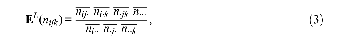
A saturated log-linear model contains sufficient statistics of effects at different levels in the contingency table. Specifically, for an array defined by three dimensions/covariates $i,j,k$ , we can specify the model as

$$\mathbf{E}(n_{\mathrm{ijk}})=\tau {\tau }_i{\tau }_j{\tau }_k{\tau }_{\mathrm{ij}}{\tau }_{\mathrm{ik}}{\tau }_{\mathrm{jk}}{\tau }_{\mathrm{ijk}},$$

where $\mathbf{E}(n_{\mathrm{ijk}})$ denotes the expected count of the $i,j,k$ cell; $\tau$ is the intercept, or the main effect of the contingency table; ${\tau }_i,{\tau }_j,{\tau }_k$ denote the marginal effects for the dimensions $i,j,k$ , respectively; ${\tau }_{\mathrm{ij}},{\tau }_{\mathrm{ik}},{\tau }_{\mathrm{jk}}$ denote the two-way interaction effects (with dimensions as above); and ${\tau }_{\mathrm{ijk}}$ denotes the three-way interaction effect over all three dimensions. (Fixing the expectation, when combined with the assumption of a maximum entropy distribution over the set of possible matrices under a Poissonian reference measure, ² fully specifies the model.)

With information of two-way margins available for the target areal unit, one could estimate the marginal effects and the two-way interaction effects. However, this is not sufficient to provide information about the three-way interaction term. Here, we approximate the three-way interaction effect for the contingency table of our target areal unit by the effect observed for its parent areal unit (treating the former de facto as a sample from the latter). This can also be viewed as a two-step process, in which we first get an expected cell input on the basis of information at the lower level, and then recalibrate it using information of the three-way interaction effect from the higher level. Formally, take ${\mathbf{E}}^L$ to be the expectation given all observable margins of the lower level (i.e., target) areal unit; then we have

$${\mathbf{E}}^L(n_{\mathrm{ijk}})={\tau }^L{\tau }_i^L{\tau }_j^L{\tau }_k^L{\tau }_{\mathrm{ij}}^L{\tau }_{\mathrm{ik}}^L{\tau }_{\mathrm{jk}}^L,$$

(1)

where ${\tau }_{·}^L$ reflects parameter estimates based on the marginals of the observed (lower level) areal unit. Now, letting ${\tau }_{\mathrm{ijk}}^H$ be the estimate of the three-way effect from $n^H$ , we use the specification

$$\mathbf{E}(n_{\mathrm{ijk}})={\mathbf{E}}^L(n_{\mathrm{ijk}}){\tau }_{\mathrm{ijk}}^H.$$

(2)

Thus, we use data from $n^H$ to fill in the “missing piece” that cannot be obtained from $n$ itself, while retaining all lower-order information from $n$ .

Because of the exponential family properties of the log-linear model, the parameters $\tau$ are easily estimated from the observed counts. The parameters describe the ratio between expected cell counts with and without the effects they represent; therefore, they are equal to 1 when absent. The general effect $\tau$ is equal to the grand mean of the contingency table, that is, ${\overline{n}}_{...}$ . The one-way marginal effects are in turn equal to the ratios between the corresponding marginal means and the grand mean. Formally,

$$\begin{array}{cc}\multicolumn{1}{c}{}& {\tau }_i=\frac{\overline{n_{i··}}}{\overline{n_{···}}}\hfill \\ \multicolumn{1}{c}{}& {\tau }_j=\frac{\overline{n_{·j·}}}{\overline{n_{···}}}\hfill \\ \multicolumn{1}{c}{}& {\tau }_k=\frac{\overline{n_{··k}}}{\overline{n_{···}}}\hfill \end{array}$$

where $\overline{n_{i··}}$ , $\overline{n_{·j·}}$ , and $\overline{n_{··k}}$ denote respective marginal means. The two-way interaction effects, in turn, are equal to the ratios of the respective two-way means to the expectations of those means arising from the respective one-way means. Formally,

$$\begin{array}{cc}\multicolumn{1}{c}{}& {\tau }_{\mathrm{ij}}=\frac{\overline{n_{\mathrm{ij}·}}}{\frac{\overline{n_{i··}}\overline{n_{·j·}}}{\overline{n_{···}}}}=\frac{\overline{n_{\mathrm{ij}·}}\overline{n_{···}}}{\overline{n_{i··}}\overline{n_{·j·}}}\hfill \\ \multicolumn{1}{c}{}& {\tau }_{\mathrm{ik}}=\frac{\overline{n_{i·k}}\overline{n_{···}}}{\overline{n_{i··}}\overline{n_{··k}}}\hfill \\ \multicolumn{1}{c}{}& {\tau }_{\mathrm{jk}}=\frac{\overline{n_{·\mathrm{jk}}}\overline{n_{···}}}{\overline{n_{·j·}}\overline{n_{··k}}}\hfill \end{array}$$

where $\overline{n_{\mathrm{ij}·}}$ , $\overline{n_{i·k}}$ , and $\overline{n_{·\mathrm{jk}}}$ denote the respective two-way means. Therefore, we may rewrite equation (1) in terms of observed counts as

$${\mathbf{E}}^L(n_{\mathrm{ijk}})=\frac{\overline{n_{\mathrm{ij}·}}\overline{n_{i·k}}\overline{n_{·\mathrm{jk}}}\overline{n_{···}}}{\overline{n_{i··}}\overline{n_{·j·}}\overline{n_{··k}}},$$

(3)

a quantity that is easily calculated.

With the first factor in hand, we now require only ${\tau }_{\mathrm{ijk}}^H$ . As with the previous cases, the three-way interaction effect is equal to the ratio of the three-way marginal mean (here, identically the count of the $i,j,k$ cell) to the expectation given the lower-order effects.

Next, we process the three-way interaction effects using information from the higher level unit. Similar to the previous derivations, the three-way interaction effect equals the ratio of the cell with the three-way interaction effect over that without the effect. Bearing in mind that all relevant counts are for $n^H$ , we have

$${\tau }_{\mathrm{ijk}}^H=\frac{\overline{n_{\mathrm{ijk}}^H}}{\frac{\overline{n_{\mathrm{ij}·}^H}\overline{n_{i·k}^H}\overline{n_{·\mathrm{jk}}^H}\overline{n_{···}^H}}{\overline{n_{i··}^H}\overline{n_{·j·}^H}\overline{n_{··k}^H}}}=\frac{\overline{n_{i··}^H}\overline{n_{·j·}^H}\overline{n_{··k}^H}\overline{n_{\mathrm{ijk}}^H}}{\overline{n_{\mathrm{ij}·}}\overline{n_{i·k}}\overline{n_{·\mathrm{jk}}}\overline{n_{···}}},$$

(4)

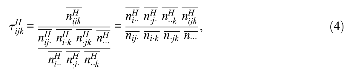
which is again easily calculated from the observed arrays. This expression for ${\tau }_{\mathrm{ijk}}^H$ makes clear that it is already “normalized” with respect to the lower-order marginals of $n^H$ ; thus, differences between $n$ and $n^H$ in such quantities do not prevent ${\tau }_{\mathrm{ijk}}^H$ from being used to model $n$ (indeed, the three-way effects by construction do not affect any lower-order marginal expectations).

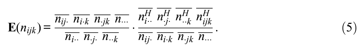
Putting these pieces together, the final target distribution is proportional to a product of Poisson distributions (a form that arises from the maximum entropy construction), whose expectations are functions of data from the target areal unit and its parent. The final target expectation for a given cell is the product of the expected distribution given the lower level information (equation 3) and the three-way interaction effect from $n^H$ (equation 4):

$$\mathbf{E}(n_{\mathrm{ijk}})=\frac{\overline{n_{\mathrm{ij}·}}\overline{n_{i·k}}\overline{n_{·\mathrm{jk}}}\overline{n_{···}}}{\overline{n_{i··}}\overline{n_{·j·}}\overline{n_{··k}}}·\frac{\overline{n_{i··}^H}\overline{n_{·j·}^H}\overline{n_{··k}^H}\overline{n_{\mathrm{ijk}}^H}}{\overline{n_{\mathrm{ij}·}}\overline{n_{i·k}}\overline{n_{·\mathrm{jk}}}\overline{n_{···}}}.$$

(5)

Imputing a Three-Way Array

We will use the target distribution specified above to find a maximum-probability array, but any three-way array imputed must match observed two-way marginals. Thus, we separate our imputation procedure into two distinct steps. First, we construct an array that satisfies the constraints imposed by the two-way marginals. Then, with this array that matches observed marginals, we optimize the array with respect to the target distribution, preserving two-way marginals. Each of these components is nontrivial. Because of the integer constraints, finding an array that matches observed marginals (a valid array) is not possible using standard techniques (e.g., the expected count array formed when performing a generalized chi-square test). Likewise, for the three-way case, optimizing the array to maximize a target distribution is a challenging task.

Constructing a Valid Array

Our algorithm to impute a target three-way array begins by finding an array that satisfies the observed two-way marginals. This component must solve an array construction problem, prior to the optimization problem discussed in the second part of the algorithm (see the section “MCMC Optimization Algorithm”). This part of the algorithm is concerned only with satisfying the two-way and integer constraints; it does not consider the target distribution for array construction.

Our strategy (detailed with pseudocode in Algorithm 1) can be broadly described as follows. Algorithm 1 also includes optimizations discussed in the section “Optimizations for the Construction Algorithm.” For a full description of the algorithm, see the section “Description of Construction Algorithm.” Our algorithm initializes an array using data from the zero-way marginal (i.e., the total array population). The population is divided equally across the array, with any remainder allocated to the first cell. This is detailed in lines 1 and 2 of Algorithm 1. This initial state ensures the total population of the array and the integer constraints are satisfied. However, it is unlikely this initial array state will satisfy the constraints imposed by the one- or two-way marginal values. We can define the deviation of our constructed array and the observed two-way marginals with the sum of the absolute values of the differences between the two-way marginals of our constructed array and the two-way marginals of the target array. We then seek to minimize this deviation.

We use a strategy of simulated annealing to produce a valid array from the initial state of our constructed array. Simulated annealing is a heuristic optimization technique designed to find the global minimum of an objective function, with minimal assumptions regarding the function and search space. This strategy will simulate moving values (individuals) between cells in the array, keeping track of deviations between the simulated marginals values and the target marginal values. A single move will decrease the value of one cell and increase the value of another cell. However, the array is not considered a valid state unless all cells in the array are nonnegative. If there is a negative value in the array after a proposed move, we draw a new move on the basis of the state of the proposed array. This process of drawing proposed changes will continue until a valid state of the array is drawn. This valid state will be proposed as a new state of our constructed array, and we compute the marginals of this array, as well as the array's deviation from the observed marginals.

The annealer will always accept moves in the array that decrease the deviation between simulated and target marginals, as these moves will bring the simulated array closer to one that satisfies the constraints of the two-way marginals. The annealer will also accept moves that increase the deviation with a probability equal to $\exp \left(\frac{D_C-D_P}{T}\right)$ , where $D_C$ is the deviation between marginals for the current array state, $D_P$ is the deviation from the marginals for a proposed array state, and $T$ is a temperature parameter. We still accept moves that increase deviation from the target marginals to prevent the annealer from finding a local minimum in the error space. However, the temperature parameter $T$ will scale the likelihood that disadvantageous moves are taken. At high temperatures, accepting moves that increase our deviation is more likely; lower temperatures make it much more difficult to accept these moves. The idea behind simulated annealing is to begin with a high temperature and allow the state of the array to vary more easily with respect to our deviation. This will help prevent the state of our array from being stuck in a local minimum of deviation. As the annealer runs, we decrease the temperature geometrically, which will minimize the deviation by the end of the annealing run. Although convergence was easily obtained in the cases studied here, it is possible that the annealer will not converge to a valid array. In this case, repeatedly restarting with a higher temperature and using a slower cooling schedule until convergence is obtained is a practical strategy. Regardless, convergence is always verifiable, as we can always determine whether our current array satisfies the target marginals (and, if not, the degree of divergence).

The annealer we describe here should produce a valid array that matches the constraints from the two-way marginals, but the basic version of the algorithm requires us to recompute the two-way marginals every time we get a new state for our constructed array. Although computing the marginals of the array once does not take a significant amount of time, computing them for every array state does add a high cost in computational time. To avoid this cost and improve the algorithm runtime, we introduce several optimizations, detailed in the next section.

Optimizations for the Construction Algorithm

The algorithm detailed in the previous section provides an array that will satisfy both the two-way marginal and integer constraints. However, because of the requirement to recompute the two-way marginals of proposed arrays, the algorithm can be expensive. To achieve better performance for larger data sets, we implement a version of the algorithm that uses a change score. Specifically, we compute the difference between the initial state of the array and the target marginals, keeping track of these persistent errors. When we move values between array cells, we then update this persistent error by subtracting a person from the departure cell of the marginals, and adding a person to the arrival cell of the marginals (rather than recalculating the marginals anew). This persistent error is equivalent to using the error metric from the previous section, but it does not require recomputing marginals.

The updated error metric will avoid the computational cost of recalculating the marginals, but it does require additional components. As noted above, we need to compute a map between the three-way array and each of the two-way marginals. This mapping will allow us to remove a person from the relevant cell of the two-way marginals and add them to the arrival cell when making a move in the three-way array. We only compute this mapping once, and can then refer to it when making moves in the three-way array. In Algorithm 1, the helper function mapIndexToMarginal will take a three-way array index and map it to the X, Y, or Z marginals, respectively.

Description of Construction Algorithm

Algorithm 1 provides pseudocode for the construction of a three-way array that matches integer and two-way marginal constraints. This algorithm uses a set of two-way marginals X, Y, and Z. The name of the marginal refers to the direction we sum across the array to produce each marginal. We also need a set of helper functions for this algorithm. The functions xMargins(a), yMargins(a), and zMargins(a) each take a three-way array and produce a two-way marginal. The function RandomInt(a,b) produces a random integer from a to b, inclusive. mapIndexToMarginal(a) takes a three-way array index and maps this index to a two-way marginal index. We use one of these functions for the X, Y, and Z marginals. Finally, numNegative(a) takes a three-way array and returns the number of negative values in the array.

Lines 1 and 2 of Algorithm 1 produce the initial state of the array. The variable $\mathrm{numTotalCategories}$ provides the number of cells in the array. Lines 3, 4, and 5 produce the deviation of the initial state of the array from the observed marginals. These values are used to compute an error metric, and will be used as a persistent deviation throughout the algorithm. Next, we specify how many arrays we will simulate with the annealer $(M)$ , and we begin simulating arrays within the loop on line 6. Lines 7 to 10 are used to initialize the state of a proposed array, as well as the deviation this proposed array would have from the target marginals.

After the deviation and array values have been initialized for our simulation, the second while loop (on line 11) begins the search for a valid array state to compare to our initial array state. Lines 12 to 16 draw two three-way array indices, $i$ and $j$ , and ensures they are different. We also produce the corresponding two-way array indices for X, Y, and Z using lines 17 to 22, which use the mapIndexToMarginal() helper function, which uses a precomputed map between three-way indices and two-way marginal indices. After we produce all the necessary indices, we move a value in the three-way array from index $i$ to index $j$ , which simply adds one to the jth cell of the array, and subtracts one from the ith cell. Lines 25 to 30 keep track of the move in the three-way array in the two-way marginals.

For this algorithm, a valid state of the array is one in which all cells are nonnegative. At the end of every proposed move, we check to see if this condition is met (lines 31, 32, and 33), and if so, immediately end the search for a new move. If any array cells are negative, we draw another move and continue until we have a nonnegative array.

With our nonnegative array, we can next compute an error metric that uses the deviations of the initial array and the deviation of the proposed array. Line 35 computes this error, which is the difference in the absolute values of the deviation summed for the initial array and the proposed array. This value would be positive if the proposed array reduces the deviation from the target marginals; it would be negative if the proposed array increases the deviation. The probability that our proposed array is accepted and becomes the current state of the array is computed on line 36; it is simply the error term divided by the temperature term, exponentiated. Lines 37 to 42 check to see if we accept the proposed array state. If we do, then the proposed array becomes the current array. Likewise, the deviations from our proposed array state would become the initial deviations for the next iteration of the loop. If the array state is not accepted, the proposal is discarded and we begin from the initial state again.

Before the loop iteration ends, line 44 cools the temperature parameter. We use a geometric cooling schedule, where the temperature parameter is multiplied by a constant for each run of the array. The final state of the array is returned on line 46, and should have minimized the difference between the marginals of the array and the target array’s marginals. In the implemented algorithm, we also check if the deviation between marginals is zero; we end the annealing process if it is. It is important to note that although this description assumed we are using this algorithm for single imputation, the algorithm will also work for multiple imputation. By fixing the cooling schedule and temperature parameters at 1, we are able to draw directly from the target distribution, which will be produced by the Markov chain.

MCMC Optimization Algorithm

The construction algorithm detailed above will produce a three-way array that satisfies the integer and two-way marginal constraints. The second component of our algorithm optimizes the three-way array’s values with respect to a target distribution, using the specification described in the section “The Target Distribution.” Our algorithm builds on the approach described by Bunea and Besag (2000) for simulating from three-way count arrays. This algorithm assumes we start with a legal imputation of the target array (i.e., an array that satisfies the set of two-way marginals and has no negative values), as well as a target distribution.

Both our algorithm and the Bunea and Besag algorithm use MCMC to simulate three-way array configurations. The transitions between states use a basic move, in which a person is moved from one cell to another in the array. However, as each state of the array is required to match the two-way marginal constraints, eight cells in the three-way array are modified in total for each basic move. Additionally, we can define the log-likelihood of a given array state under the target distribution, which we will denote $l(n)$ , where n is a three-way array. For two arrays, a current and proposed array, the probability for the Markov chain to accept the proposed move is $\exp (l(n\prime )-l(n))$ , where $n$ is the current array state, and $n\prime$ is the proposed array state. Because the basic move preserves all lower-order marginals, validity of an array produced by this method is guaranteed (i.e., any array generated from a valid starting point will always be a valid array).

We modify Bunea and Besag’s algorithm by using simulated annealing. In the construction component of this algorithm, we used annealing to optimize the state of an array to minimize deviation from the observed marginals. As our goal in this part of the algorithm is to find the most likely configuration of the algorithm under the target distribution, we can use simulated annealing for better single imputation quality. The addition of simulated annealing is straightforward, and only requires us to modify the acceptance probability with a temperature parameter. As with the construction algorithm, the temperature parameter will scale the probability that the optimization algorithm accepts proposed arrays that are less likely under the target distribution. Higher temperature values (above 1) will increase the likelihood that less likely array configurations are accepted. Likewise, as temperatures approach zero, the probability of accepting lower-probability array configurations also goes to zero. A fixed temperature at 1 will accept new array states by exactly evaluating the likelihood within the target distribution. A benefit of updating this algorithm to use simulated annealing is that the algorithm can be run in both single and multiple imputation modes. In single imputation mode, the temperature would be set above 1, and the cooling schedule would be set below 1. However, as mentioned above, by setting the temperature and cooling schedule to 1, we would draw directly from the target distribution, which enables multiple imputation.

Optimization Algorithm Description

Algorithm 2 provides pseudocode for the optimization of a three-way array with respect to a target distribution corresponding to the maximum entropy distribution on $n$ conditional on $\mathbf{E}(n)$ and the two-way marginals. We need several helper functions for this implementation. First, we use a helper function doBasicMove(n), which takes a three-way array as an input, and moves someone from one cell in the array to another, maintaining all two-way marginals. As discussed above, this basic move modifies eight cells of the three-way array (for more details, see Bunea and Besag 2000). We also use the helper function numNegative(n), which takes a three-way array as an input, and outputs the number of negative values in the array. Finally, the helper function numNegativeOne(n) takes a three-way array as an input and outputs the number of negative ones in that array.

Algorithm 2.

Impute a Three-Way Crosstab.

Require: target expectations $\mathbf{E}(n)$ , array state $n$ , initial temperature $T$ , decay parameter $c=0.94$

01: while $M>0$ do

02:  while $L>0$ do

03:   $n\prime \leftarrow \mathrm{doBasicMove}(n)$

04:  while numNegativeOne $(n\prime )=1$ do

05:    $n\prime \leftarrow$ doBasicMove $(n\prime )$

06:  end if

07:  if numNegative $(n\prime )>1$ then

08:    next

09:  else $\{\mathrm{numNegative}(n\prime )=0\}$

$\mathrm{randomNum}\leftarrow$ Uniform $(0,1)$

#Accept the proposed array with probability equal to the ratio of probabilities of proposed:current arrays

11:   if $\mathrm{randomNum}<$ min $(1,\exp (($ l $(n\prime )-$ l $(n))/T)))$ then

12:     $n\leftarrow n\prime$

13:   end if

14:  end if

15:    $L-=1$

16:  end while

17:   $M-=1$

#Cool the chain

18:   $T\leftarrow T*c$

19: end while

20:  $\mathrm{return}(n)$

Implementation of our algorithm relies on a Markov chain that cools as the annealer runs. The total length of the Markov chain is $M*L$ , where M is the number of times we cool the Markov chain, and L is the number of iterations we run the Markov chain at each temperature. At each step of the Markov chain, we start by proposing a basic move on the target three-way array n (line 3). $n\prime$ , the proposed three-way array, will match all two-way marginal and integer constraints. Next, we follow the Bunea and Besag algorithm by checking the number of negative values (specifically negative ones) in $n\prime$ . If there is exactly one negative one in the array, we draw a new basic move from $n\prime$ ; we continue to do so until either there is more than one negative value in $n\prime$ , or $n\prime$ becomes a nonnegative array. If $n\prime$ is an array with more than one negative value, we discard the proposal, keeping the original state of the array. However, if $n\prime$ is a nonnegative array, we compute the ratio of the likelihoods for $n\prime$ and $n$ (in log space) under the target distribution, and divide this log-likelihood by a temperature parameter (line 11). When exponentiated, this is the probability the proposed array is accepted as the next state of the Markov chain.

Every $L$ iterations of our Markov chain, we cool the chain. Like the construction algorithm, we use a geometric cooling schedule for this algorithm, multiplying the temperature of the annealer by a constant every $L$ iterations. As the temperature of the annealer decreases, the Markov chain will accept proposed states that are lower likelihood under the target distribution less often than at higher temperatures.

Validation of Imputed Data Quality

The previous sections provided algorithms for construction and imputation of three-way count arrays with targeted characteristics. Next, we describe the test imputations and metrics we use to validate the quality of population data imputed using this approach. Our validation tests use U.S. census data on population distributions, using several levels of geographic aggregation. We also use two validation metrics to determine data quality.

Data Used for Validation Runs

We use data from the 2010 U.S. census to assess the quality of our imputation technique. The U.S. decennial census published complete three-way population distributions at several levels of geographic aggregation. The census uses a geographic hierarchy for their data products, with census blocks aggregating into census tracts, which themselves aggregate into counties. ³ We consider the three-way distribution of race, gender, and ethnicity within each geographically defined subpopulation (i.e., count data for each three-way category). Ethnicity has two categories, non-Hispanic and Hispanic. Gender also uses two categories, male and female; race has seven categories. ⁴ Given the national scale of the census, these distributions provide a large data set for us to test our imputation.

We perform two imputation studies to validate the approach. The first uses U.S. census data across the entire United States, specified at the county and tract levels. Here, target distributions are defined using three-way distributions at the county level. At the tract level, we use the two-way observed marginals for our target array. Full three-way distributions are publicly available at the tract level, which allows us to directly validate the quality of the imputation. We impute the three-way distribution of race, ethnicity, and gender for each of the 73,057 tracts in the United States. We perform single imputation and multiple imputation for each tract, comparing true values against imputed counts.

Our second imputation study involves analysis of a social outcome (exposure to crime), using data specified at the tract and block levels. We specify a target distribution using full, three-way arrays available at the tract level, and use marginal two-way arrays that were published at the census block level of aggregation. We chose to only impute the three-way arrays for one U.S. state (California), which contains 710,154 census blocks. Comparison of analysis at the tract level on actual versus imputed data provides another check on imputation quality. Although we cannot directly validate block-level imputation (because the three-way marginals are not available), we use this for an illustrative case study (see the section “Case Study for Quality Checking”).

Imputation Parameters

For both validation samples, we use the same settings for array construction and optimization. The imputation calculations were completed on the same machine, using the same computing resources (facilitating timing comparisons).

First, we detail the parameters used for construction of a valid array. For each array we construct, we simulate up to 1 million array states ( $M$ in Algorithm 1). We allow for up to 1,000 moves to find a new valid array state ( $K$ in Algorithm 1). We initialize our temperature parameter $T$ to be 10 times the error rate (deviation from the marginals) produced by the initial state of the array. In practice, all arrays produced by the implementation of Algorithm 1 were found to match the two-way and integer constraints, indicating these parameters are sufficient for the heuristic optimization to succeed in finding valid array states.

Next, in the optimization component of the algorithm, we use a Markov chain of length 50,000 for each array. We cool this chain every 1,000 iterations, for a total of 50 annealing steps. The initial temperature parameter $T$ is set to 10, with a cooling parameter $c$ of 0.94. This allows the annealer to accept less likely array states more readily for half of the Markov chain, with the second half of the Markov chain behaving more strictly as a hill climber, seeking the maximum likelihood array state.

When doing multiple imputation, we fix both the temperature and the cooling parameter at 1 (i.e., we fix the algorithm at the target distribution, with no cooling). This allows us to draw directly from the distribution of array states that is specified by the target distribution and the marginal constraints. We use a thinning parameter of 1,000 and a burn-in parameter of 1,000, which were found to be adequate for convergence. In seeding the Markov chains for the multiple imputation draws, we initialize the optimization portion of our method with a draw from the single imputation mode of the algorithm. We do this to ensure the Markov chain will burn-in, by starting it at a mode of the target distribution.

Each of our imputation studies was performed on an Intel Xeon E5-2599 V4 central processing unit (CPU). As the three-way array that is present for any areal unit does not depend on any other areal unit, this problem is trivially parallelizable. Thus, we used 30 cores for each imputation. We also introduce several special cases where we can directly solve the state of the three-way array. In the first case, there is no population in the array. Second, we can directly solve the “one-hot” case, or arrays in which there is only one cell with any population. We can solve these arrays using only information from the two-way marginals, trivially imputing the array.

Metrics for Assessing Data Quality

We use two main methods for the assessment of data quality. Both metrics require observed data as a baseline. We rely on the tract-level imputation described above, as the full three-way tract arrays are published in addition to the two-way marginal data. Our first metric for assessing data quality relies on an error metric, and can be assessed on an individual array basis. We also provide a metric for assessing quality that depends on stable performance in a downstream analysis.

Error-Based Metric for Data Quality

The first metric we use to asses data quality measures the degree that an imputed three-way array departs from its observed values. In other words, this accuracy metric measures how many people are mismatched between a simulated and observed array. Our error metric, $E$ , is defined as $E=\sum _i|O_i-I_i|$ , where $O$ is the observed array for an areal unit, $I$ is the imputed array for the same areal unit, and the sum is over entries of the array. This error metric simply represents the number of people who are misallocated by the imputation.

For purposes of expressing this error metric in a standardized manner, we divide $E$ by the number of people present in the areal unit, which normalizes the error values to a range between 0 and 1. (In tracts with zero population, we define the metric to be zero.) This value is referred to as $E_R$ , and describes the percentage of the tract that has been misallocated. Low values of this error metric indicate high-quality imputed data.

We compare the errors produced by our algorithm to error rates produced by several other approaches. The first alternative we compare to is one described by Bunea and Besag, in which there is no simulated annealing, and we simply use a Metropolis algorithm to take a single draw from the distribution defined at the higher level of geography. In this case, error rates should be broadly similar—if the Markov chain is burned in correctly, a random draw from that distribution is relatively likely to be from a high-probability region—but with higher excursions because the algorithm will occasionally select plausible but low-probability arrays. This provides a point of comparison for the annealing algorithm, which uses the same target distribution but attempts to provide a maximum-probability array.

Next, we examine the case where we use the expected values provided by the target distribution as the final imputed values. These expected counts are produced using the log-linear framework described in the section “The Target Distribution,” which incorporates two-way data from the target level of geography with three-way patterns present at the higher level of geography. Because the log-linear model is not constrained to satisfy integer constraints, it is expected to accumulate numerous errors; however, it incorporates distributional information, and (being easy to compute) is an obvious practical alternative.

Finally, to examine the improvement produced by simulating the distribution of possible three-way states under the target distribution, we also examine the error rates when using the array generated by the construction algorithm as the final imputed value. This array will be “valid,” in that it satisfies both integer constraints and the known two-way marginals, but not otherwise adjusted. We examine this case to better understand how the space of three-way arrays may be constrained by the two-way marginals. This technique would also omit all data from the higher level of geography, so we can examine how only incorporating the local demographic effects (i.e., the two-way marginal constraints) may produce different arrays from the observed data.

Case Study for Quality Checking

Although direct error assessment is the most natural way to evaluate imputation quality, it does not speak directly to downstream effects on subsequent analysis: relatively poor imputation may prove adequate when downstream analyses are robust, but sensitive analyses may require very high degrees of imputation accuracy. Such sensitivity inevitably depends on the analysis involved; here, we use a case study involving a spatially heterogeneous outcome—exposure to crime in one’s vicinity—as a plausible example of how errors may or may not affect substantive conclusions. Specifically, we carry out our analysis at the tract level using observed and imputed data, allowing us to compare results obtained in the two cases. For this purpose, we use single and multiple imputation, allowing us to compare the performance of both estimators at recovering observed-data results. Finally, as an illustrative procedure, we repeat our data analysis at the block level. Although not suitable for validation (as we do not have block-level observations), this analysis provides an example of how the imputation approach might be used in a realistic case, and how pushing analysis to finer levels of geographic detail can potentially affect our substantive conclusions.

Our case study examines how exposure to crime near one’s home is related to one’s demographic characteristics. Crime is heterogeneously distributed, making members of some groups more likely than others to be exposed; such exposure may, in turn, feed concerns about neighborhood safety, willingness to access local affordances, and stress. To examine this association, we use crime data obtained from police agencies for the Southern California Crime Study (SCCS). The SCCS researchers made an effort to contact each police agency in the Southern California region and request address-level incident crime data for six part 1 Uniform Crime Reports categories: homicide, aggravated assault, robbery, burglary, motor vehicle theft, and larceny. These data come from crime reports officially coded and reported by the police departments and provide locations of crime incidents around 2010 covering about 83 percent of the population in a five-county area (Los Angeles, Orange, Riverside, San Bernardino, and San Diego). Crime events were geocoded for each city separately to latitude/longitude point locations using ArcGIS 10.2, and subsequently aggregated to various units such as blocks and tracts. The average geocoding match rate was 97.2 percent across cities, with the lowest value at 91.4 percent. These data have been used in several prior studies (Kubrin and Hipp 2016; Kubrin, Hipp, and Kim 2018).

We use the number of violent crime events that took place (homicide, aggravated assault, robbery) and compute the average over three years (2009–2011) to smooth year to year fluctuations. Prior literature shows that one’s exposure to crime is affected by many demographic features, including the ones we have imputed in this article (Alba et al. 1994; Logan and Stults 1999; McNulty 1999). The actual form of this relationship has not been closely examined, however, particularly at the level of small areal units, which are needed to avoid averaging across areas with different crime rates. Thus, using observed and imputed data at the census tract level, we specify a saturated linear regression model (i.e., main effects, two-way interaction terms, and three-way interaction terms). Additionally, we specify the same models at the census block level, only using imputed data. We examine the block-level model to compare whether the effects are similar to those of the tract-level model. At the tract level, the mean number of crime events in the data is 42.38 events, with a minimum of zero and a maximum of 666 events. At the block level, we use an additional buffer around each areal unit. This buffer has a radius of 1 km. The mean number of crime events for the block level data is 112.22 events, with a minimum of zero and a maximum of 2,234 events.

The census geographies we use here are adjacent levels of the census spatial hierarchy. Census tracts compose counties and are often relatively large. For tracts represented in the SCCS, the average tract population in 2010 was 4,604 people. Although tracts can provide an overview of population distributions across space, the census block level is much more granular (often about the size of a city block). The average population for a census block in the area represented by the SCCS is approximately 80 people; the five counties have an average population of 3.765 million.

To compute one’s exposure to crime (i.e., the response term for this model), we use the number of crime events that occur in a given areal unit, using data from the SCCS. From this number of crime events, we consider a group’s exposure to crime in that areal unit as $C_{\mathrm{ijk}}=E{p}_{\mathrm{ijk}}$ , where E is the number of violent crime events that occur for that areal unit, and $p_{\mathrm{ijk}}$ is the proportion of the total number of people in a three-way race, ethnicity, gender category (for the entire sample) that are present in the areal unit. These values are summed across all areal units to produce an exposure for each of the groups. This exposure functionally behaves as a weighted average of crime exposures in each areal unit. We then predict this exposure using dummy variables for each race, ethnicity, and gender category, as well as all two- and three-way interaction effects using these terms. The White, non-Hispanic male category is used as a reference group for these regressions.

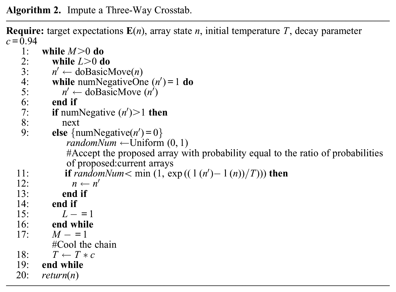
Given that these fully-specified models are not common in the literature, we present three hypotheses about the nature of the relationship between the explanatory factors and one’s exposure to crime, motivated by more general notions of cumulative, intersectional, and saturated mechanisms of disadvantage. These hypotheses are schematically represented by Figure 2. We consider individuals as belonging to one or more social categories, reflecting, for example, race and gender. Members of a given social category may be, on average, particularly likely to be exposed to specific underlying sources of disadvantage; some such sources may be unique to specific categories, and others may be shared by members of multiple categories. Schematically, Figure 2 depicts social categories as boxes, each of which contains a set of “keys” that “unlocks” particular sources of disadvantage (here indicated by color). An individual belonging to only one social category receives the keys—and hence the sources of disadvantage—for that category. When an individual belongs to multiple categories, they inherit the keys from each category to which they belong. The consequences of this can vary, leading to several hypothetical scenarios.

Figure 2.

Schematic depiction of the ways overlapping social category memberships can lead to different degrees of realized disadvantage.

Our first scenario, represented by the subadditive row of Figure 2, occurs when the sources of disadvantage for an individual’s social categories overlap. In this case, having multiple memberships in disadvantaged groups provides more disadvantage than being a member of a single category, but not as much as the independent combination of both groups. Here, the sources of disadvantage saturate, and their effect on the individual is subadditive.

Our second scenario, represented by the additive row, occurs when there is no overlap in the sources of disadvantage for the categories to which an individual belongs. Here, the total disadvantage is simply the sum of the disadvantage for each category.

Finally, in our third scenario (the superadditive row) we consider the possibility that some sources of disadvantage require “keys” from multiple categories to unlock. In this case, the total disadvantage for multiple group memberships can exceed the sum of the group disadvantages, because a joint member is affected by both the union of the two group sources and additional sources of disadvantage that arise from comembership. This is often discussed within the context of intersectionality (Crenshaw 1990), with the notion that belonging to multiple disadvantaged groups can have a substantially greater effect than the independent effects of each membership alone.

In the context of exposure to crime, it is plausible that sources of disadvantage associated with gender, race, and ethnicity could correspond to any of these three scenarios. To quantify this, we specify an additivity index, which we use to categorize the relationship for each of our three-way categories included in the model. This index can be defined by

$$A=\frac{{\beta }_{\mathrm{ijk}}}{a+{\beta }_i+{\beta }_j+{\beta }_k+{\beta }_{\mathrm{ik}}+{\beta }_{\mathrm{jk}}+{\beta }_{\mathrm{ij}}},$$

where $a$ is the intercept term, and the $\beta$ terms are the regression coefficients for the one-, two-, and three-way effects. If the three-way effect in this term is zero, then the index will also be zero, which implies a purely additive relationship. Likewise, if the sign of the total two-way effects and three-way interaction term are the same, then the index will be positive, indicating a superadditive relationship. Finally, if the numerator and denominator are of different signs, this index would be negative, which indicates a subadditive relationship. In the rare case where the total two-way effect (denominator) is zero, we define $A$ to be zero.

The magnitude of the index is also informative. Usually, we would expect $A$ to be between −1 and 1, which indicates the three-way effect is smaller in magnitude compared with the rest of the effects. However, in the event that $A$ is greater in magnitude than −1 or 1, this indicates the three-way effect outstrips the combined two-way effects, and would be able to flip the sign of the total effect.

Tract Imputation Results

Next, we describe the results of the imputations discussed above, evaluating the overall quality of the imputed arrays. Imputing all 73,057 tracts took 7 hr, 33 min, and 49 seconds on 30 cores of an Intel Xeon E5-2599 V4 CPU. As the tract-level three-way arrays in the United States are known, we can directly compare the imputed three-way arrays with the observed data. We use the error metric specified in the section “Error-Based Metric for Data Quality.”

Array Approximation Results

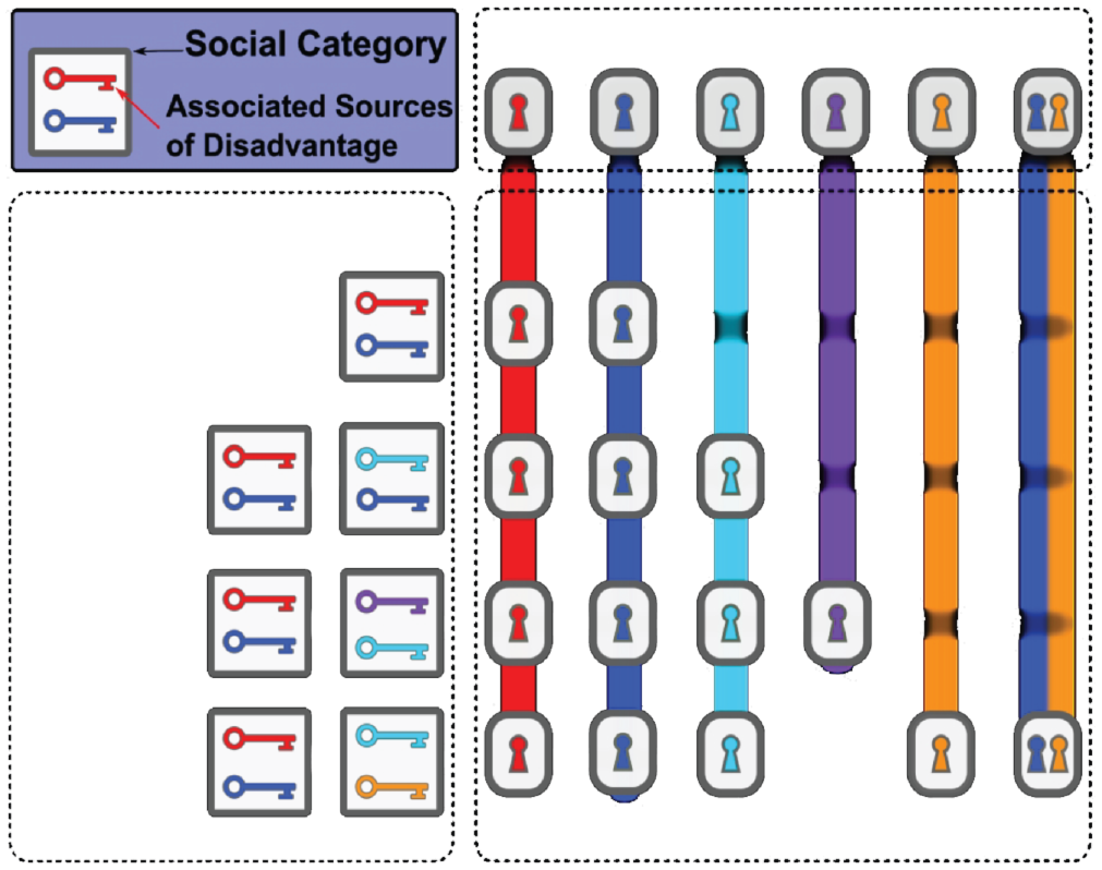
This error metric provides support for the quality of the data imputation. Figure 3 describes the distribution of relative errors, showing that most tracts have a very low error rate. Given that the mean relative error is 0.8 percent and the 97.5th percentile of the error is 2.5 percent, this imputation schema produces three-way arrays that are excellent proxies for the observed data (with error rates at or below error rates in the census itself; Khubba, Heim, and Hong 2022).

Figure 3.

A histogram of relative errors.

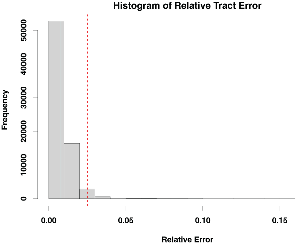
We compare these error rates to the rates obtained by the other procedures described in the section “Error-Based Metric for Data Quality.” We find that drawing directly from the target distribution (using Bunea and Besag’s algorithm without simulated annealing) produces very slightly elevated error rates compared with the ones produced by our updated algorithm. The mean error rate for all tracts in the United States is 0.009 (0.9 percent), and the 97.5th percentile of the error is 0.0283 (2.83 percent). The arrays produced by this algorithm are produced by the same process that we use for multiple imputation, which we will show produces similar qualitative results to the single imputation case when doing downstream data analysis. We thus conclude there is some gain from annealing to find the mode of the target distribution (versus using an arbitrary draw), but error rates are not very sensitive to this aspect of the algorithm.

Next, when using the expected counts produced by the log-linear models (for our target distribution) as the imputed arrays, we see noticeably elevated error rates. The mean error rate is 0.0124 (1.24 percent), and the 97.5th percentile of this error distribution is 0.0396 (3.96 percent). These error rates are still relatively low, but they are roughly 50 percent higher than the annealed imputation method, and the estimates do not satisfy integer constraints (making them unsuitable for some applications).

For the third case, where we simply construct a valid three-way array that conforms to the integer and marginal constraints, we would expect the error rates to be significantly higher than when we use simulated annealing to produce the most likely three-way array under the target distribution. Indeed, the mean error rate produced by this imputation is 0.047 (4.7 percent), and the 97.5th percentile of the error is 0.158 (15.8 percent). This case provides an interesting point of comparison, as it shows the space of three-way arrays is significantly constrained by the two-way marginals, but despite this, significant improvements are still made through the optimization components of the algorithm. To further visualize the differences between the imputations described here, we plot the error histograms in full in Figure 4.

Figure 4.

Histograms describing the error rates for the imputations described in this section.

Overall, these results suggest that although constraints are powerful, incorporating distributional target information is still important for getting high-quality approximations. When this is done, optimization to ensure a mode is selected (versus a random draw from the target) is helpful, but less vital. This also implies that our approach is not extremely sensitive to annealing performance, which may be useful in settings for which the cost of high-quality annealing runs is a concern.

Results for Downstream Analysis

In addition to direct approximation error, we also use the case study described in the section “Case Study for Quality Checking” to evaluate data quality. Our case study examines the effects of disadvantaged social category membership on exposure to crime. As we are using three-way arrays to examine this relationship, we are particularly interested in the three-way coefficients from the regression specified above. Figure 5 shows the coefficients for the observed data model and the imputed data model. For the observed data model, the means and variances are directly computed from 1,000 bootstrapped samples of areal units. We use a standard bootstrap sampling design for the observed data model.

Figure 5.

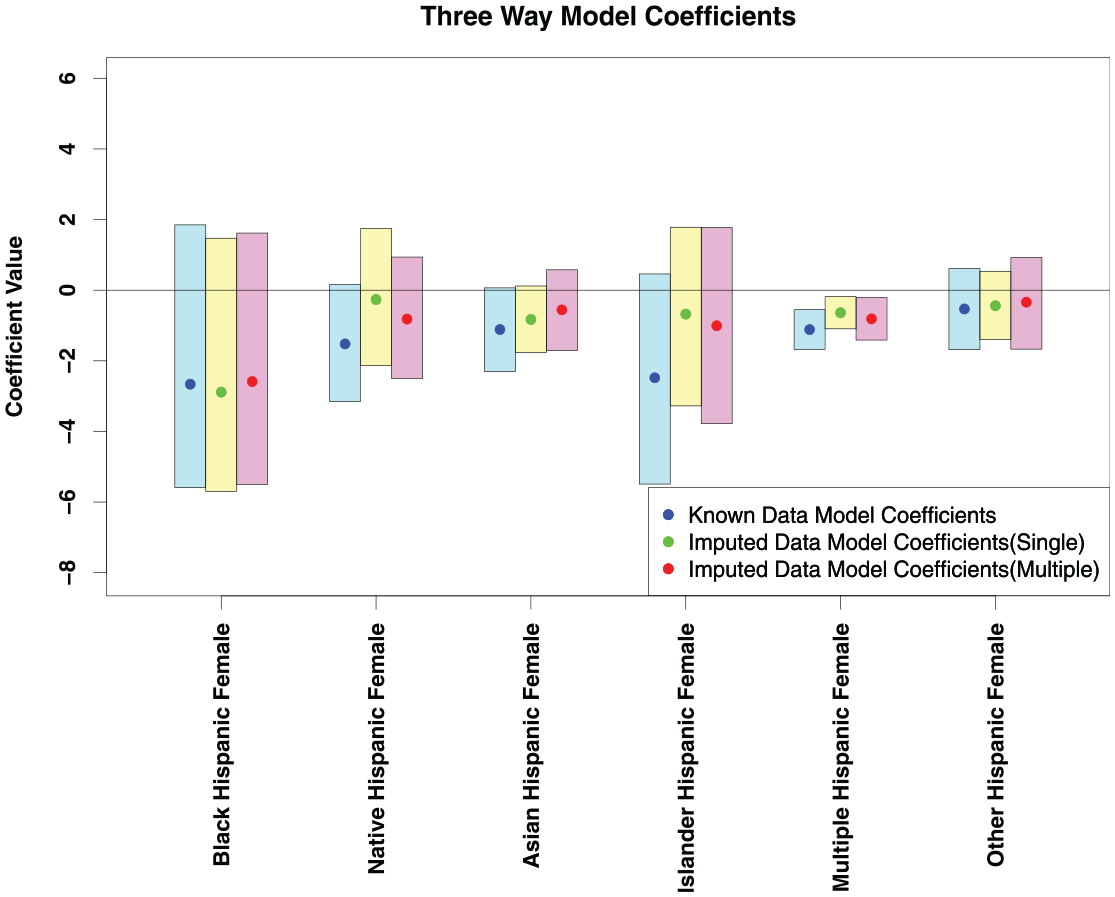
A plot of three-way effects.

For the imputed data model, we examine the effect of using the algorithm in single imputation mode versus multiple imputation mode. In single imputation mode, we draw a single array for each areal unit. Then, we sample areal units using the standard bootstrap design. In the multiple imputation mode, we use a slightly different sampling method. For each of the 2,000 bootstrapped samples, we draw a set of arrays from the distribution defined by our target distribution. The Markov chains used to draw from this distribution were seeded with a draw from a single imputation run of the algorithm to ensure the chains were burned in adequately. Then, we draw $n$ arrays from that areal unit, where $n$ is the number of times that areal unit has been drawn for that bootstrap sample. We then use the quantile method to compute the distribution of each coefficient.

The three-way coefficients from Figure 5 almost all overlap with zero, indicating mostly additive effects. In addition, the simulated and observed distributions of three-way coefficients all have significant overlap with each other. A researcher would obtain similar qualitative results from interpreting the observed and simulated models (i.e., the effects significantly different from zero are the same). This indicates that qualitatively, the simulated arrays are similar in nature to the observed arrays, and would not introduce significant error into downstream analysis. Additionally, although the single imputation produces coefficients that tend to be slightly closer to zero, both single and multiple imputation modes produce similar results to the observed data model.

We also examine the patterns in the coefficients reported in Figure 5 with respect to their additivity indices. For each coefficient reported from the analysis done with the bootstrapped samples from the observed three-way arrays, we compute the additivity index from the section “Case Study for Quality Checking.”Figure 6 reports the distribution of these additivity indices. As expected from a cursory examination of the coefficients in Figure 5, the majority of coefficients exhibit an additive pattern. For the Black, Hispanic female and Pacific Islander, Hispanic female coefficients, there are some cases of subadditivity present, but for the most part, the three-way coefficients describe an additive relationship between disadvantaged category membership and exposure to crime at the tract level. Notably, we find no sign of systematic superadditivity at this level of aggregation.

Figure 6.

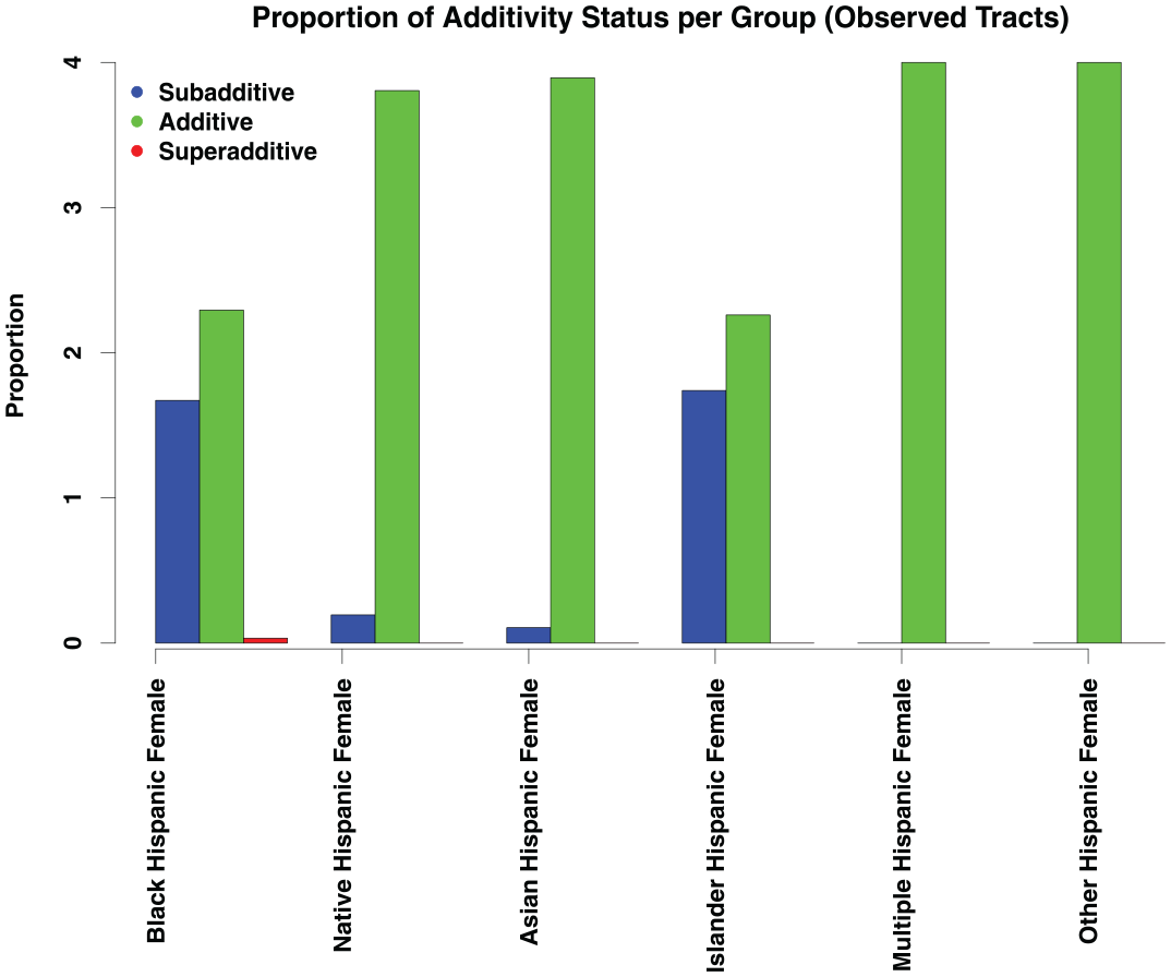
Additivity indices for each of the three-way categories in the model across 2,000 bootstrap iterations.

Block-Level Imputation Results

The tract-level analysis suggests additive effects are predominant, but this could be an artifact of aggregating over locally heterogeneous units. Although the full data needed to replicate the observed-data analysis at the block level is not available, we can do so using our imputation scheme. For a single imputation, we imputed the 710,145 census blocks in California on 30 cores of an Intel Xeon E5-2599 V4 CPU in 12 hr, 53 min, and 42 seconds. We hypothesize that the higher areal unit/second imputation rate is likely due to the lower population of census blocks compared with census tracts. There are also more census blocks than census tracts that can be trivially solved (see the section “Imputation Parameters”). The full three-way arrays at the census block level are not available, so we are unable to compute the same error metrics that we use for the census tract imputation.

Given the imputed block-level arrays, we once again examine the relationship between gender, ethnicity, and race on exposure to crime. We apply the same basic procedure as in the tract-level case study. However, rather than measuring crime in the specific block (which is too small a unit of analysis to provide a reasonable notion of exposure), we measure crime in a 1-km buffer around each focal block. Once again, we use multiple imputation to get a set of potential arrays for each areal unit, drawing from the target distribution specified at the tract level.

The three-way effects from the block-level exposure to crime are summarized in Figure 7. We used 500 bootstrapped samples from the crime and areal unit data to compute the simulation intervals for this plot. The patterns in these coefficients generally match the patterns from the tract-level analysis, but the magnitude of these coefficients is much greater. None of the three-way coefficients intervals contain zero, representing significant three-way effects. We use the same multiple imputation sampling as described above to generate these estimates.

Figure 7.

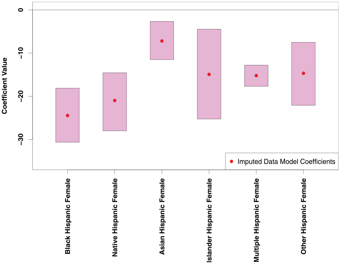
Estimates of three-way coefficients at the census block level.

As the observed effects are consistently negative, we expect there is less of a strongly additive pattern at the block level. Figure 8 depicts the patterns in the additivity index for the three-way coefficients. Almost all the coefficients exhibit a strongly subadditive pattern, with only the other race, Hispanic female and Asian, Hispanic female categories having some additive indices. We thus find that, at fine spatial scales, the relationship between exposure to crime and disadvantaged group memberships is subadditive, implying that the sources of disadvantage associated with group memberships overlap. This runs counter to the common intuition that disadvantage compounds across social categories, but it is mechanistically sensible: many things can lead to living in poor housing, or having a large number of potential offenders nearby, but once one acquires such a source of disadvantage, there is a limit to how much additional impact it can have. Thus, the sources eventually saturate, with diminishing marginal effects. This nonlinear effect is lost when data are aggregated to the tract level, as would be necessary without the ability to impute at the block level.

Figure 8.

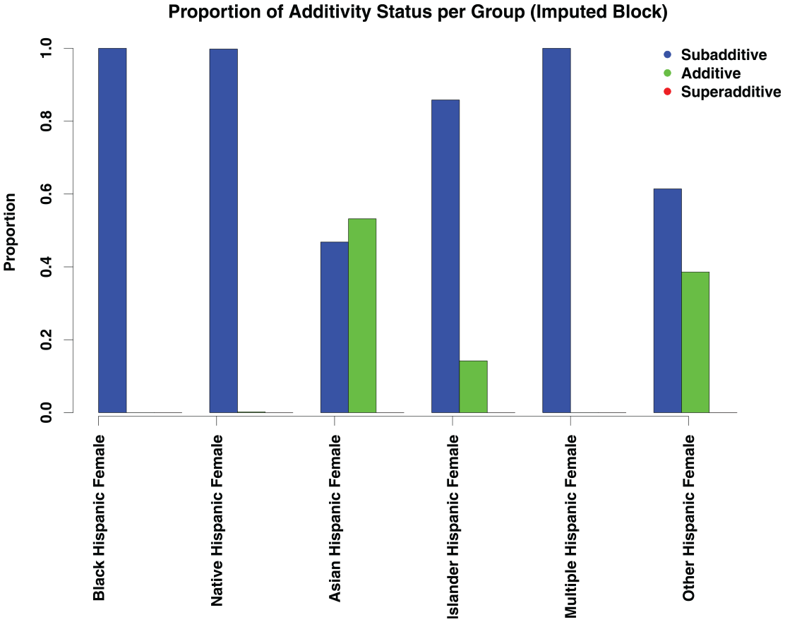
Additivity indices for the three-way block coefficients.

Although the pattern of additivity indices is different between the block- and tract-level analyses, we note that the general pattern of the coefficients matches. We do not see radical differences across scales, but rather subtle variations that can be obscured by averaging. As noted, however, those variations can lead to distinct substantive conclusions about the nature of disadvantage in crime exposure.

Discussion

We implemented and tested an imputation framework for nested areal units, showing it produces high-quality data for three-way arrays that contain count data. The algorithm specified in this article should produce high-quality data for arrays in which all entries are nonnegative integers. Likewise, we are able to leverage data at a higher level of geographic aggregation to optimize the configuration of an imputed array to what we expect the correlations between array cells to be.

With the recent push in many social science fields for measures constructed at smaller geographic scales, along with the limited availability of some data at such small geographic scales, our imputation algorithm may be applicable in a range of settings. For example, our case study showed a generally similar pattern in crime exposure for residents of different demographic groups whether measured in census tracts or the smaller spatial unit of blocks, but we saw sharper and stronger patterns when using the smaller geographic units. Given the spatial segregation of residents at varying spatial scales, measuring such effects at smaller geographic scales is arguably substantively important for addressing such research questions. The spatial averaging that occurs when aggregating to larger geographic units risks obscuring the patterns we were able to observe after imputing the data to blocks.

Implementation of this algorithm represents a substantial step forward in three-way array imputation, especially with the constraints we described, but the problem of imputing high-order arrays is still difficult. For example, Bunea and Besag (2000) claim that for the three-way crosstab imputation problems without two-way marginal constraints (i.e., with independent one-way margins), the Monte Carlo method is amenable, yet this remains a scenario where the formulae are not yet derived and the algorithms are not yet implemented. They also point out that their algorithm is specific to the three-way array case, and although the basic move could, in theory, be adapted to a higher-order array, the problem cannot be solved in a “plug and play” fashion. A new transition set must be derived for higher-order arrays, as the transition rule used here is specific to the three-way case (and, in general, each order requires a new set of basic moves, associated with its respective symmetry group). Integrating higher-order marginal constraints into models for simulating high-order array data would also be a valuable next step in this line of research.

Another open question in this area is the provable irreducibility of the underlying Markov chain used for the multiple imputation case. The construction algorithm provided here is verifiable, and the optimization and imputation algorithms guarantee the result is margin-preserving, but the basic move of Bunea and Besag has not been proved to be irreducible in all cases. Their original paper proves irreducibility for any $I\times J\times K$ array such that one of the dimensions has cardinality 2. Irreducibility is thus ensured for the cases studied here, or any other population data using, for example, a two-class sex tabulation. Subsequent work by Lee (2018) provides a proof for the $3\times 3\times K$ case, as well as simulation studies suggesting the property is preserved for cardinalities $4\times 4\times 4$ and higher. It thus appears likely the property holds for all three-way arrays, although this is still unproven. Failure of irreducibility would imply that the Markov chain would not explore the entire state space of possible arrays, thus possibly (1) finding a point estimate that suboptimally captures three-way correlations or, (2) in the multiple-imputation case, providing an imperfect approximation to the target array distribution. (It would not, however, lead to invalid imputations.) Care should thus be exercised when using this method for multiple imputation on arrays that violate the cardinality conditions, when a high level of precision is required.

The model we used in this article to simulate three-way array data is highly scalable. For small areal unit estimation, our imputation scheme does not require information on adjacent units’ imputed values, so each areal unit can be estimated independently. This has substantial computational benefits, as large sets of areal units can be imputed in parallel, which provides a significant decrease to overall runtime. We were able to simulate three-way distributions for all tracts in the United States, as well as all census blocks in California, in less than 24 hr, showing the algorithm can be used in other very large regions. Both the construction and optimization problems contribute to runtime, so it is likely that arrays with lower population would increase imputation speed, as the construction algorithm will converge more quickly with fewer people.

Release of small areal unit data often reflects a “tug-of-war” between advocates of openness, transparency, and data quality (on the one hand) and privacy (on the other). Each faction cites a range of arguments in its favor (often with a certain degree of zealotry), and we here limit ourselves to commenting on implications for the imputation problem. Three-way imputation applied to valid data may or may not allow data identification at a given level of confidence, depending on cell counts; for the scenario studied here, high-confidence identification must come from the two-way marginals, as the higher-order correlation structure is both estimated and approximate. Techniques such as differential privacy can be used by data collectors to design perturbed marginals that provide guaranteed bounds on identifiability, and algorithms such as those shown here may be useful for verifying the results of such constructions (and ensuring they still lead to valid arrays). Similar validation applications are possible for privacy-preserving techniques based on, for example, areal unit aggregation (whereby units are merged until they no longer permit identification beyond the specified level of confidence). Given that data-perturbing methods such as differential privacy pose significant data quality concerns, another use for this type of imputation method is to ensure the perturbed data yield imputed arrays that are still appropriate for downstream analysis. Particularly given the importance of neighborhoods, blocks, and other small units for social processes related to social disadvantage, obfuscation methods that induce systematic bias in small-scale structure have the potential to negatively affect policy-relevant research affecting vulnerable communities. We hope obfuscators will leverage imputation and related methods to help verify their modifications will not have such downstream effects.

The imputation techniques introduced here could also be extended in several ways. First, there could be additional spatial dependencies among the areal units. For this case, the algorithm could be extended by generating a target distribution from both the areal unit immediately higher in the spatial hierarchy from the target unit, and from that unit’s neighbors. A natural approach is to estimate ${\tau }_{\mathrm{ijk}}^H$ using a spatial smoother at the level of higher-order units, then using this (rather than the ${\tau }_{\mathrm{ijk}}^H$ based only on the parent unit) for lower level imputation. Directly incorporating autocorrelation at the lower level is also possible, but would require a more complex, multilevel approach and would be less amenable to parallelization. Both are potentially fruitful directions for further work.

Likewise, this technique could also be extended to cases where the areal units are not perfectly hierarchical. The most obvious direction to extend the algorithm would be similar to the extension described for using multiple parent geographies. In this case, it may make sense to average the correlation structure of parent geographies that overlap with the target areal units. A more radical proposal of this type is suggested for cases in which complete three-way information is available for some units, but only two-way information is available for others. In this case, an interesting option is to train a kernel learner (Scholkopf and Smola 2001) or similar predictive algorithm to predict the lower level ${\tau }_{\mathrm{ijk}}$ coefficients from observed marginals and other spatial and contextual data; the trained algorithm can then be used to predict ${\hat{\tau }}_{\mathrm{ijk}}$ directly, as opposed to using ${\tau }_{\mathrm{ijk}}^H$ as a proxy. Although kernel learning suggests itself because of its interpretation in terms of a similarity function, other methods could also be used.

On a final, substantive note, our sample application to exposure-to-crime data suggests disadvantage in this context is largely subadditive: notably, we do not see the superadditive effects often presumed (but less often tested) in sociological discussions of intersectionality. This subadditivity is largely masked at higher levels of geography (although we do not see evidence of superadditive effects there, either). Although it is possible this is peculiar to the case of crime exposure, the mechanistic interpretation discussed here would suggest the phenomenon may be much more common. A more systematic investigation of when and how often disadvantage is additive, subadditive, and superadditive across different contexts and for different types of disadvantage would greatly illuminate theory in this area, and may also inform policy interventions. Regardless, our findings reinforce the value of fine-grained spatial data for accurate assessment of local social processes.

Conclusion

We specified and demonstrated an algorithm for imputing three-way array data within a hierarchically nested context. This imputation problem is challenging, as it is constrained by the two-way marginal structure of the array, an integer constraint, and needing to be optimized with respect to higher-order array data. We provide a scalable, robust technique to impute these three-way arrays that relies on MCMC and simulated annealing strategies.

In a test imputation of all tracts in the United States, simulated data from our algorithm produced remarkably low error rates. At the tract level, we observed a mean allocation error of approximately 0.8 percent, with nearly all tracts having errors below 2.5 percent. Such errors are better than or comparable with error levels in the census itself (Khubba et al. 2022), suggesting imputation is unlikely to be a dominant source of error in subsequent analyses. Likewise, in a case study that examines three-way categories exposure to crime, we found that both imputed and observed data produced similar conclusions about the relationship between disadvantaged category membership and exposure to crime. Combined, both of these metrics show that the imputed arrays are very similar to observed arrays, and can be used in downstream analyses without introducing significant error.

As sketched herein, there is considerable room for further work on the imputation of higher-order array data embedded in spatial hierarchies. With the proliferation of these nested data structures, methods that allow the use of data at low levels of geographic aggregation where data may be incomplete are particularly valuable.