Sage Journals: Discover world-class research

Abstract

Respondent-driven sampling (RDS) is used to measure trait or disease prevalence in populations that are difficult to reach and often marginalized. The authors evaluated the performance of RDS estimators under varying conditions of trait prevalence, homophily, and relative activity. They used large simulated networks (N = 20,000) derived from real-world RDS degree reports and an empirical Facebook network (N = 22,470) to evaluate estimators of binary and categorical trait prevalence. Variability in prevalence estimates is higher when network degree is drawn from real-world samples than from the commonly assumed Poisson distribution, resulting in lower coverage rates. Newer estimators perform well when the sample is a substantive proportion of the population, but bias is present when the population size is unknown. The choice of preferred RDS estimator needs to be study specific, considering both statistical properties and knowledge of the population under study.

Keywords

respondent-driven sampling disease prevalence sampling social networks validation

Probability-based sampling is the gold standard for unbiased estimation of the prevalence of a trait or disease in a population. However, when the target population is marginalized, or otherwise hidden among the general population, no sampling frame exists. Respondent-driven sampling (RDS) (Heckathorn 1997), a chain-referral technique, is a well-established method for estimating disease prevalence in these hidden populations by leveraging information about the underlying social network. RDS estimators can account for the increased likelihood of sampling people with larger social networks, the tendency of people to cluster by disease status (homophily), and differences in number of personal connections for different groups (relative activity) to allow asymptotically unbiased and accurate estimation of trait or disease prevalence.

Early estimators were based on the assumption that recruitment could be approximated by a Markov chain. A key insight was that the likelihood of inclusion in an RDS sample is inversely proportional to the number of connections a person has with other members of the target population, that is, their personal network degree. Salganik and Heckathorn (2004) developed the RDS-I or SH estimator, an early estimator of prevalence in RDS studies. This estimator infers the prevalence of disease in a population from the cross-group ties observed in the sample and each respondent’s reported degree. A subsequent estimator, developed by Volz and Heckathorn (2008), the RDS-II or VH estimator, is an inverse-probability weighted estimator and remains the most commonly reported estimator of RDS prevalence (Abdesselam 2019). Both of these estimators have the advantage of relying solely on sample data, without requiring additional knowledge of the target population.

Gile’s (2011) successive sampling (SS) estimator was the first to model a true RDS process, of sampling without replacement, and was shown to be more accurate than RDS-II when the sample size is not a small fraction of the population size. Fellows (2019) suggested an improvement on Gile’s SS estimator: on the basis of a homophily configuration graph (HCG), this estimator iteratively estimates network degrees and the proportion of cross-group ties until the prevalence estimate converges. Several studies have investigated the performance of RDS-specific estimators for trait prevalence (Baraff, McCormick, and Raftery 2016; Fellows 2019; McCreesh et al. 2012; Verdery et al. 2015; Wejnert 2009). However, as Gile et al. (2018) noted, none has identified a uniformly best estimator. Recently, Spiller et al. (2018:40) stated that the SS estimator is superior to the RDS-II estimator unless the population size is “dramatically underestimated,” and Fellows (2019) provided evidence that the HCG estimator is less biased than earlier estimators when the sample size is large relative to the population and the population size is known.

As Goel and Salganik (2010) noted, performance of RDS estimators is often poor because of the high variability of the resulting estimates. This variability is also linked to the sampling process; sampling with replacement results in larger design effects than sampling without replacement (Baraff et al. 2016; Fellows 2019; Goel and Salganik 2010). Variance estimation is also a challenge in RDS studies, and prior work has reported lower than expected coverage rates (e.g., Baraff et al. 2016; Goel and Salganik 2010; McCreesh et al. 2012; Spiller et al. 2018). Spiller et al. (2018) conducted a systematic review of commonly used variance estimators in RDS and reported the best coverage with Gile’s SS estimator coupled with a bootstrap estimate of variance, and unacceptably low coverage for the naive sample proportion. Baraff et al. (2016) proposed tree bootstrapping over the RDS recruitment trees to calculate confidence intervals around the RDS-II estimator, and Green, McCormick, and Raftery (2020) showed the consistency of the method, but to our knowledge this method has yet to be implemented in practice. To date, all validation work has been conducted on binary outcomes and with relatively small networks.

The absence of large networks makes it difficult to validate RDS prevalence estimators. Spiller et al. (2018) created synthetic networks with N = 10,000 on the basis of the properties of the National HIV Behavioral Surveillance system surveys (2009–2012) conducted by the Centers for Disease Control and Prevention in the United States using exponential random graph modeling (ERGM). Gile (2011) also used ERGM to simulate networks but modeled a maximum population size of N = 1,000, which is likely small for many populations in urban areas. Synthetic networks generated using ERGM can have a specified level of homophily, relative activity, and mean degree, and tend to produce Poisson-like degree distributions (Crawford 2016). Fellows (2019) sampled from a Poisson distribution for network degree in his simulations evaluating RDS estimators. A recent survey of 53 RDS samples encompassing more than 36,000 participants indicated that reported degree from every RDS sample was considerably more skewed than a Poisson distribution and was approximately log-normal across all sample types (migrants, men who have sex with men, drug users, sex workers) and geographies (North America, India, Papua New Guinea) (Avery et al. 2021). The effect of degree distribution on estimator accuracy has not yet been examined.

Although estimation methods have been extended to categorical outcomes, validation of RDS estimators has focused on binary outcomes, likely because large networks with categorical outcomes with which to perform validation are rare. The National Longitudinal Study of Adolescent to Adult Health (Harris and Udry 2021) and Facebook College (Rozemberczki, Allen, and Sarkar 2021) data sets have been used extensively in RDS validation (Abdesselam 2019; Abdesselam et al. 2020; Fellows 2019; Goel and Salganik 2010; Handcock, Gile, and Mar 2014; Spiller et al. 2018; Verdery et al. 2015). However, as Spiller et al. (2018) noted, these data sets are “unlike the hidden populations networks through which RDS coupons are typically passed” (p. 30). These populations are relatively small (N = 1,249 in National Longitudinal Study of Adolescent to Adult Health, N = 1,259 in Facebook College), and instead of reported network degree, a truncated proxy is used, further restricting the degree range. In summary, our goal is to extend the existing literature on estimator validity by incorporating observed real-world reported network degrees into larger simulated networks and to explore estimator performance on categorical outcomes using both real-world and synthetic networks.

Description of RDS Data

Properties of RDS Samples

The goal of RDS sampling is to estimate the trait prevalence, π. Sampling begins with the selection of seeds (often about 10), usually purposefully chosen from the population of interest. Each seed is given a fixed number of coupons (usually 2–5) with which to recruit other members of the population. Participants complete a survey to determine (1) their outcome status ( $y_{i} = 1$ for those with the trait of interest, $y_{i} = 0$ otherwise) and (2) the number of other members of the target population they know, referred to as their network degree, $d_{i}$ .

Researchers also often ask questions to ascertain whether the participant belongs to the target population. From the recruitment coupons, researchers can link each participant with their recruiter. From a total population of $N$ , $n$ participants are sampled. In the underlying population, the sum of the network degrees is twice the number of network edges $\sum_{i = 1}^{N} d_{i} = 2 T$ , where, in the situation of two groups $T = T_{00} + T_{11} + T_{01}$ are the connections among those with $y_{i} = 0$ (T₀₀), among those with $y_{i} = 1$ (T₁₁) and between groups (T₀₁), respectively. Throughout this article, we refer to the mean degree of those with ( $\bar{d_{1}}$ ) and without ( $\bar{d_{0}}$ ) a trait and use Gile’s (2011) notation:

\bar{d_{0}} = \frac{\sum_{i = 1}^{N} d_{i} (1 - y_{i})}{\sum_{i = 1}^{N} (1 - y_{i})}, \bar{d_{1}} = \frac{\sum_{i = 1}^{N} d_{i} (y_{i})}{\sum_{i = 1}^{N} (y_{i})}, \bar{d} = \frac{\sum_{i = 1}^{N} (d_{i})}{N}

Population homophily quantifies the relative likelihood of within-group to between-group connections (i.e., the degree to which birds of a feather flock together). Definitions for homophily are varied in the literature, but we chose the definition consistent with the RDS package available for R (Handcock et al. 2021), such that

H = \frac{π (1 - π) \bar{d_{0}} \bar{d_{1}} N}{\bar{d} T_{01}}

Relative activity (ω) describes the difference in the connectivity of the groups and is simply the ratio of the mean degree between groups:

ω = \frac{\bar{d_{1}}}{\bar{d_{0}}}

Simulated Networks

Figure 1 provides an overview of the study work flow. We created networked populations of size $N = 20, 000$ with varying levels of trait prevalence, homophily, and relative activity. Nodes corresponding to study participants were indexed from $i = 1, 2, 3, \dots N$ . We set trait prevalence, $π,$ to either 0.20 to enable comparisons with Fellows (2019) or 0.05 to model rarer traits. We drew reported network degree, $d_{i}$ , with replacement, from one of two distributions: (1) actual reported degree compiled from 17 samples of men who have sex with men (Lachowsky et al. 2019; Solomon et al. 2019; Weikum et al. 2019) or (2) Poisson distributed with mean of 6, for comparison with results from Fellows (2019). These degree distributions are illustrated in the bottom row of Figure 2. Each node, $n_{i}$ , was assigned $d_{i}$ edge-ends, corresponding to network degree. For a fixed-degree distribution, trait prevalence, and level of homophily, we were unable to precisely fix the relative activity. We therefore chose to contrast equal activity with elevated activity.

Figure 1.

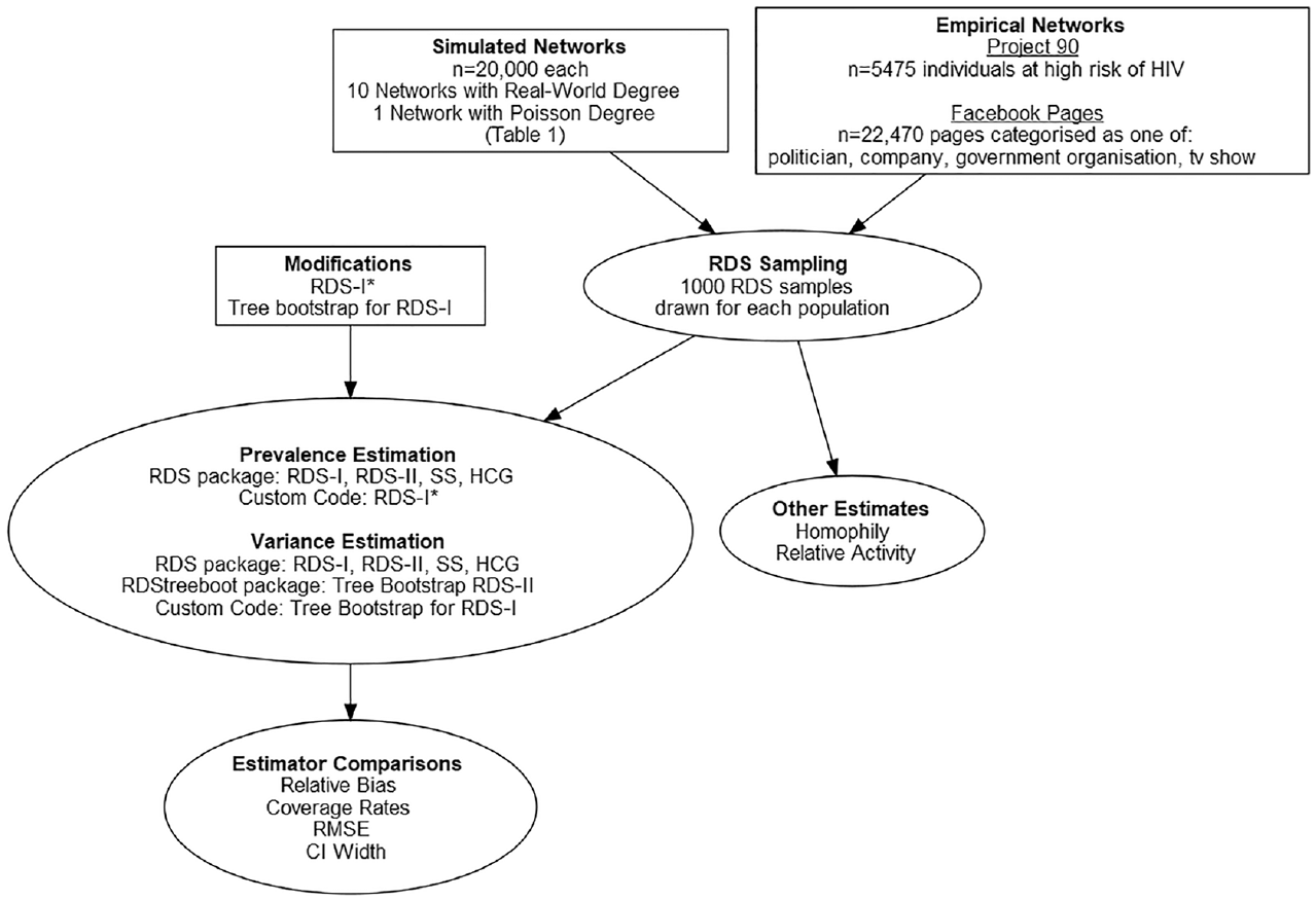
Overview of study work flow.

Figure 2.

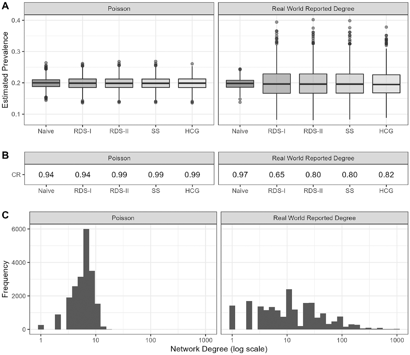
Comparison of estimator performance between population with Poisson-distributed degree (left) and degree drawn from real-world reported degrees (right). Panel A: Distribution of estimated prevalence from simulated samples. Panel B: Coverage rate across simulated samples. Panel C: Distribution of network degree in the simulated population.

We assigned group membership ( $y_{i}$ ) depending on the desired level of relative activity as follows:

To produce a population with equal activity ( $ω = 1$ ): for group $1$ , randomly select $n_{1} = π N$ nodes and assign them $y_{i} = 1$ (representing nodes with the trait). For all other nodes, set $y_{i} = 0$ (group $0$ ).

To produce a population with elevated activity ( $ω > 1$ ): for group $1$ , randomly sample $0.75 π N$ nodes from nodes with $d_{i} > d_{q 50}$ and the remaining $0.25 π N$ nodes from nodes with $d_{i} \leq d_{q 50}$ , where $d_{q 50}$ refers to the median degree across all groups. For all other nodes, set $y_{i} = 0$ (group $0$ ).

We used the following process to network population nodes:

Population homophily levels of no homophily (H = 1), moderate homophily (H = 1.25), and strong homophily (H = 10) were investigated. The number of between group ties was calculated as

T_{10} = \frac{\sum_{i = 1}^{N} d_{i} (y_{i}) \sum_{i = 1}^{N} d_{i} (1 - y_{i})}{H \sum_{i = 1}^{N} d_{i}}

The resulting number of ties within groups is then $T_{00} = \sum_{i = 1}^{N} d_{i} (1 - y_{i}) - T_{10}$ and $T_{11} = \sum_{i = 1}^{N} d_{i} (y_{i}) - T_{10}$ .

Unconnected edge-ends from group $0$ were randomly drawn and connected. If a self-connection formed, it was discarded and the draw repeated. This process was repeated until there were $T_{00}$ ties within group $0$ .

The previous step was repeated for group $1$ .

The remaining edge-ends from groups $0$ and $1$ were randomly drawn and connected to form cross-group ties.

For all ties $t_{01}$ , reciprocal ties were created, $t_{10},$ so that the graph was undirected.

In this manner, we set the exact degree distribution, trait prevalence, and homophily for a synthetic network with no self-loops to mimic a real-world network.

Empirical Data

Project 90

The Project 90 study collected full network data on a community of individuals at high risk for human immunodeficiency virus transmission. Originally published by Potterat et al. (2004), we used the partial data set reported by Goel and Salganik (2010). These data have subsequently been used in a number of papers assessing RDS methods (e.g., Baraff et al. 2016; Crawford 2016; Fellows 2019; Goel and Salganik 2010). The data set is available from the Office of Population Research (https://opr.princeton.edu/archive/p90/) and contains information on 15 characteristics of 5,475 individuals. Previous work has focused on the single largest connected network. Here we include all individuals and perform RDS sampling whereby if recruitment stalls, additional seeds are added. RDS estimators assume a connected network, but this is untestable in practice and our goal was to replicate real-world conditions as much as possible.

Facebook Pages

The Large Facebook network (Rozemberczki et al. 2021) is a network of 22,470 verified Facebook sites (network nodes), classified by Facebook as politicians, companies, television shows, or government organizations. The sites were connected by 171,002 mutual “like” linkages, which serve as the network edges. Data were extracted through the Facebook Graph API in November 2017 as part of the multiscale attributed node embedding project and are available at GitHub (https://github.com/benedekrozemberczki/MUSAE). Unlike the Project 90 participant characteristics, the four page categories are mutually exclusive and represent a single categorical variable.

Additional Populations Based on Preliminary Findings

Preliminary findings from the simulated and empirical networks prompted further study. In light of large variability in the RDS-I and HCG estimates of the categorical trait in the Large Facebook network under strong homophily, we modified additional simulated networks to create a categorical trait for further testing of estimator performance. We added a categorical variable to populations 6 and 11 from Table 1 (strong homophily) on the basis of the original binary outcome as follows:

Table 1.

Characteristics of the Simulated Populations

Population	DegreeDistribution	Prevalence	Homophily	RelativeActivity	Observed ω	ObservedH
1	Poisson	.20	No homophily	Equal activity	.97	.99
2	Real world	.05	No homophily	Equal activity	1.16	1.00
3	Real world	.05	Moderate homophily	Equal activity	.83	1.24
4	Real world	.20	No homophily	Equal activity	.98	1.00
5	Real world	.20	Moderate homophily	Equal activity	.96	1.24
6	Real world	.20	Strong homophily	Equal activity	.97	9.32
7	Real world	.05	No homophily	Elevated activity	1.66	1.00
8	Real world	.05	Moderate homophily	Elevated activity	1.52	1.23
9	Real world	.20	No homophily	Elevated activity	1.71	1.00
10	Real world	.20	Moderate homophily	Elevated activity	1.78	1.24
11	Real world	.20	Strong homophily	Elevated activity	1.63	9.51

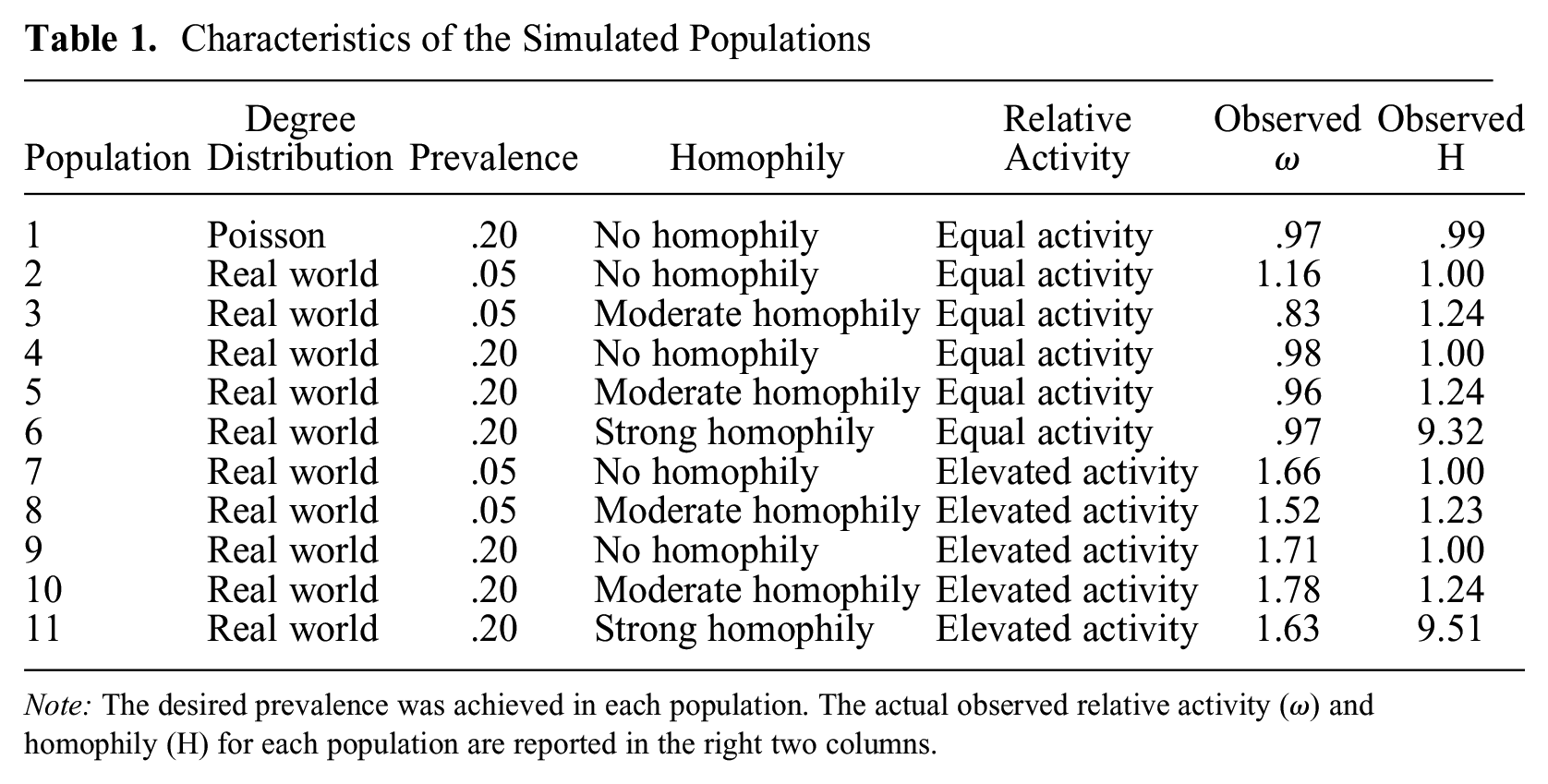
Note: The desired prevalence was achieved in each population. The actual observed relative activity (ω) and homophily (H) for each population are reported in the right two columns.

Group a: randomly selected from group 0 with probability 0.25.

Group b: all others from group 0.

Group c: randomly selected from group 1 with probability 0.25.

Group d: all others from group 1.

RDS Sampling Process

For each population (simulated and empirical), we drew 1,000 RDS samples to represent real-world conditions.

Ten seeds were randomly selected from the network nodes. This method was chosen to reflect the fact that researchers often purposely choose seeds to best reflect a population and are unlikely to choose seeds biased with respect to the trait of interest. Furthermore, in Fellows’s (2019) study examining these same estimators, biased seeds had little effect on estimator performance.

Available neighbors were defined as connected nodes not already in the sample (i.e., sampling without replacement).

For each node, between 0 and 3 recruits were sampled from the available neighbors with probability (0.35, 0.15, 0.4, 0.1). These probabilities are based on the observed number of recruits reported across many RDS samples (unpublished data).

Steps 2 and 3 were repeated until a sample size of 5,000 was reached; we obtained smaller samples of n = 500 by taking the first 500 recruits.

If recruitment stopped, then 10 new seeds were added and recruitment continued from step 2.

Statistical Analysis

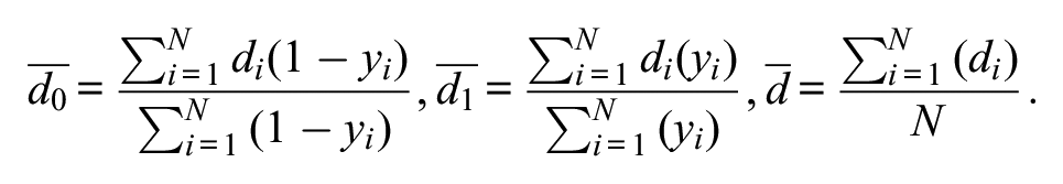
We investigated the naive sample proportion, RDS-I, RDS-II, Gile’s SS estimator, and the HCG estimator. The RDS package version 0.9-2 (Handcock et al. 2021), available in the R statistical programming language (R Core Team 2021), was used for all parameter estimation. For the HCG estimator, we used sampling wave as a proxy for recruitment time, because this information is reliably available to researchers in practice. We also evaluated a modified RDS-I estimator in an attempt to resolve situations in which extreme estimates of 0 or 1 were produced. This situation arises when there are no observed recruitment links from one group to another. From Salganik and Heckathorn (2004), the RDS-I estimator of the prevalence of condition $A$ , for a binary outcome with possible values $A$ and $B$ is

{\hat{π}}_{A} = \frac{d_{B}^{*} C_{B A}}{d_{A}^{*} C_{A B} + d_{B}^{*} C_{B A}}

where $d^{*}$ are sample-based estimates of mean degree, and $C_{AB}$ and $C_{BA}$ are the probability of recruitment from group A to B and from B to A, respectively, calculated from the observed group-group recruitment matrix ( $t_{ij}$ ). If either $C_{AB} = 0$ or $C_{BA} = 0$ , the resulting estimates will be 0 or 1. When an outcome is binary, it is unlikely, especially in large samples, that no cross-group recruitments will be observed. However, with rare traits or categorical outcomes, the likelihood increases. To overcome this limitation, we created a slightly modified estimator (RDS-I*) by replacing zero values in the off-diagonal elements of the observed group-group recruitment matrix with 1, thereby preventing extreme values in the Markov transition probabilities ( $C_{AB}$ and $C_{BA}$ ).

We assessed accuracy of the estimators using the root-mean-square error (RMSE). Estimator coverage was calculated as the proportion of samples for which the 95 percent confidence interval contained the true population proportion. Estimator bias was calculated as a ratio of the difference between the mean point estimate across samples and the population parameter to the population parameter ( $bias = \frac{\bar{\hat{π}} - π}{π}$ ). For each sample, we also estimated homophily using the RDS package, and relative activity using both the ratio of mean degree between groups and the ratio of the Salganik-Heckathorn estimates of mean degree used in the RDS-I estimator (Salganik and Heckathorn 2004).

Because the SS and HCG estimators require knowledge of the population size, which is often unknown, we computed three variations of each of these estimators: using the known, true population size ( $N$ ), using half the population size ( $N / 2$ ), and using twice the population size ( $2 N$ ). We examined further sensitivity of the HCG estimator to misspecification of $N$ for cases where HCG was the preferred estimator.

For the Facebook Pages data, in addition to the confidence intervals calculated in the RDS package using the analytic variance estimators, we used the tree bootstrap to calculate confidence intervals around the RDS-I and RDS-II estimators. The RDStreeboot package (Baraff 2016) provides these confidence intervals around only the RDS-II estimator. We used the package to draw tree bootstrap samples and then modified the code to produce confidence intervals around the RDS-I* estimator. To limit calculation times in these large networks, we drew 100 tree bootstrap samples to calculate the confidence intervals. It is more common to use 2,000 bootstraps, but it was necessary to reduce this substantially in a simulation setting.

Results

Table 1 details the achieved population-level homophily and relative activity for each of the simulated populations. A survey of RDS studies indicated that degree distributions in many real-world populations are approximately log-normally distributed (Avery et al. 2021). To allow comparison with previous literature and estimate real-world performance, Figure 2 shows the effect of personal network degree distribution on estimator variability for populations with equal relative activity and no homophily. Log-normally distributed degrees produce RDS-adjusted estimates with a small negative bias, more variability, and lower coverage rates than Poisson-distributed degrees. The coverage rate for RDS-I is near nominal levels when degree is Poisson distributed, but lower than the other estimators for real-world reported degrees.

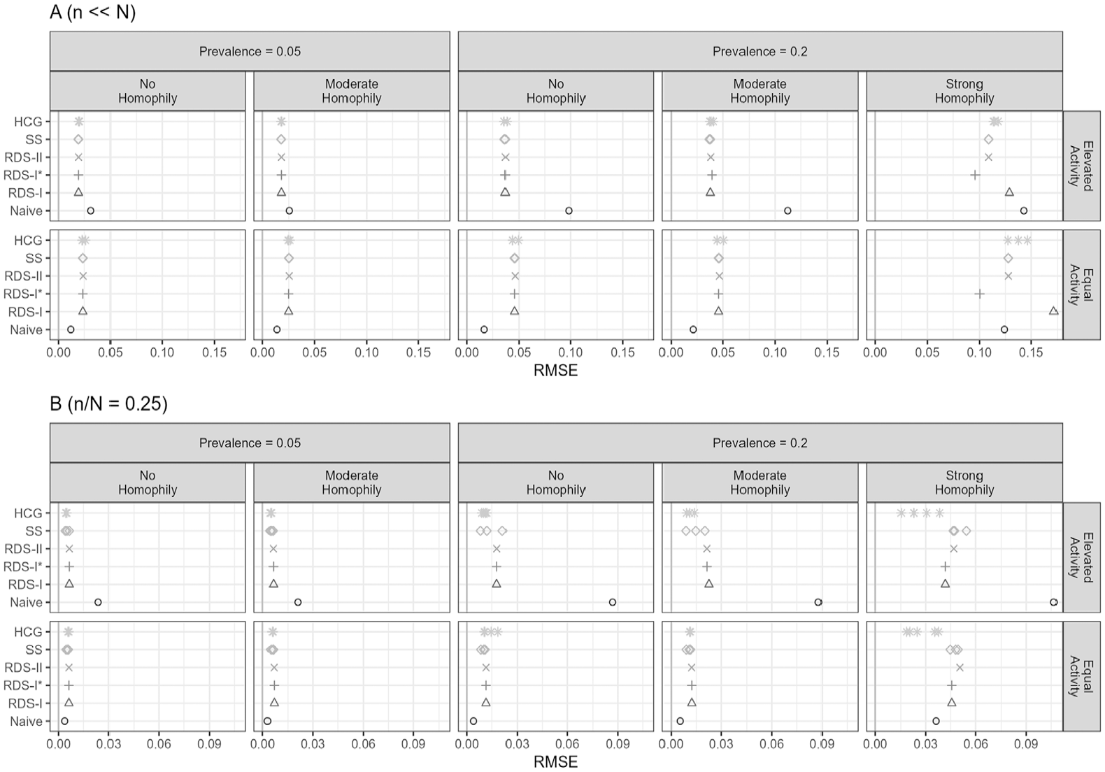
Figure 3 illustrates the RMSE for the simulated populations with n << N (A) and n/N = 0.25 (B). We calculated the SS and HCG estimates with three different possible population sizes: the correct size ( $\hat{N} = N$ ), half the true population size ( $\hat{N} = N / 2$ ), and double the true population size ( $\hat{N} = 2 N$ ). The HCG estimator performed well at these levels and was superior to the SS in the presence of homophily, so we performed additional simulations exploring $\hat{N} = 4 N$ and $\hat{N} = 10 N$ . All RDS estimators perform similarly in most circumstances, with differences arising under conditions of strong homophily. When strong homophily is present, the adjusted RDS-I* estimator has the lowest error when n << N, and when (n/N = 0.25) the HCG has the lowest error, even when the population size is misspecified. Note that the accuracy of RDS-II is on par with that of HCG.

Figure 3.

RMSE of estimators across simulated populations. Dichotomous traits with small sample fraction (A) and large sample fraction (B).

Figure 4 presents relative bias for the same scenarios. In general, bias is small across all RDS estimators when activity is equal between trait groups and in the absence of homophily. The presence of either homophily or differential activity increases bias, as does low trait prevalence. In the presence of strong homophily, all estimators are biased and there is no clearly preferred estimator. When elevated activity is present, the SS and HCG estimates are biased toward 1 when the population size is underestimated and toward 0 when the population size is overestimated.

Figure 4.

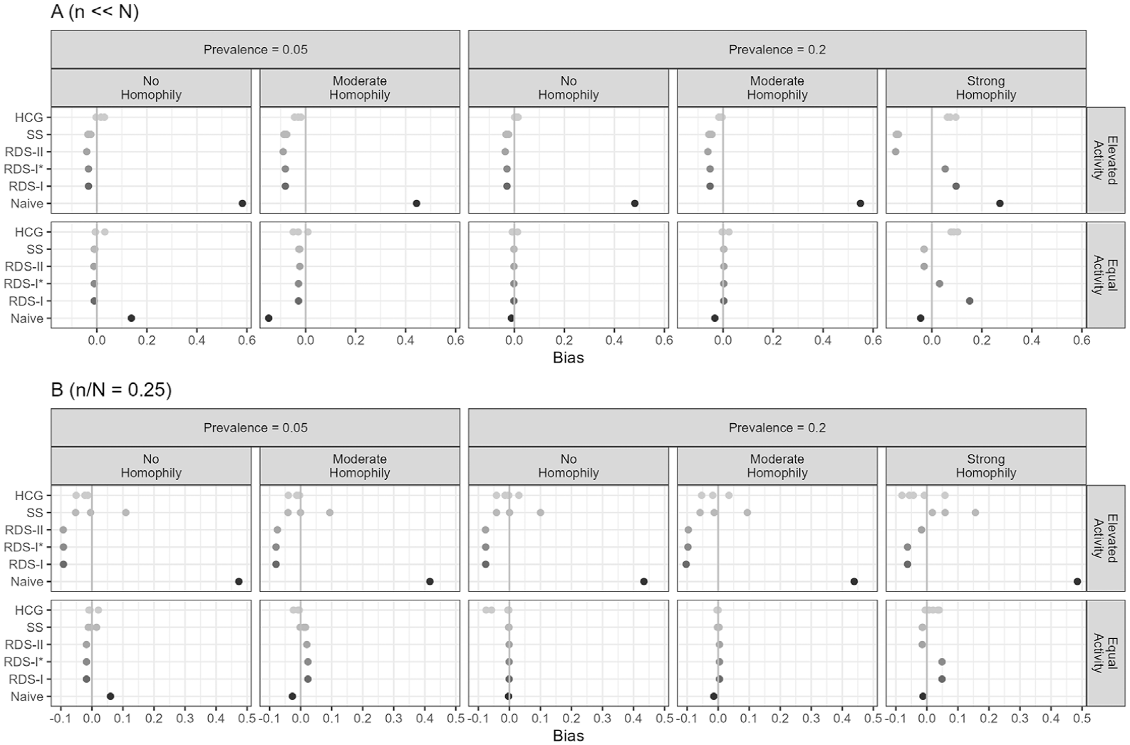
Relative bias of estimators across simulated populations. Dichotomous traits with small sample fraction (A) and large sample fraction (B).

Tables S1 and S2 in the online supplement provide the coverage rate and median confidence interval width for the simulated populations. Although none of the RDS estimators achieve the nominal coverage rate, the RDS-II estimator has relatively good coverage and does not depend on knowledge of the population size. When the sample is a large proportion of the population and strong homophily exists, coverage of all estimators is poor. The tree bootstrap has increased coverage rate, but the width of the resulting confidence interval is double or even triple those of other estimators. Tables S3 and S4 in the online supplement provide the relative bias and RMSE of the RDS estimators for the simulated populations.

Project 90 Network

Figure S5 in the online supplement illustrates the degree distribution of the Project 90 and the Large Facebook Pages networks. Figure 5 presents sample estimates for the Project 90 data, and Table 2 presents the accuracy, bias, and coverage. Population properties, which vary by trait, are given in Table S6 in the online supplement. The RDS estimators perform similarly and have improved accuracy over the naive sample mean, which exhibits large bias for most traits. The RDS-II estimator has the lowest error except for the sex work client trait, where the HCG estimator (assuming accurate knowledge of the population size) is preferred. None of the estimators could capture the prevalence of drug dealers or non-White ethnicity.

Figure 5.

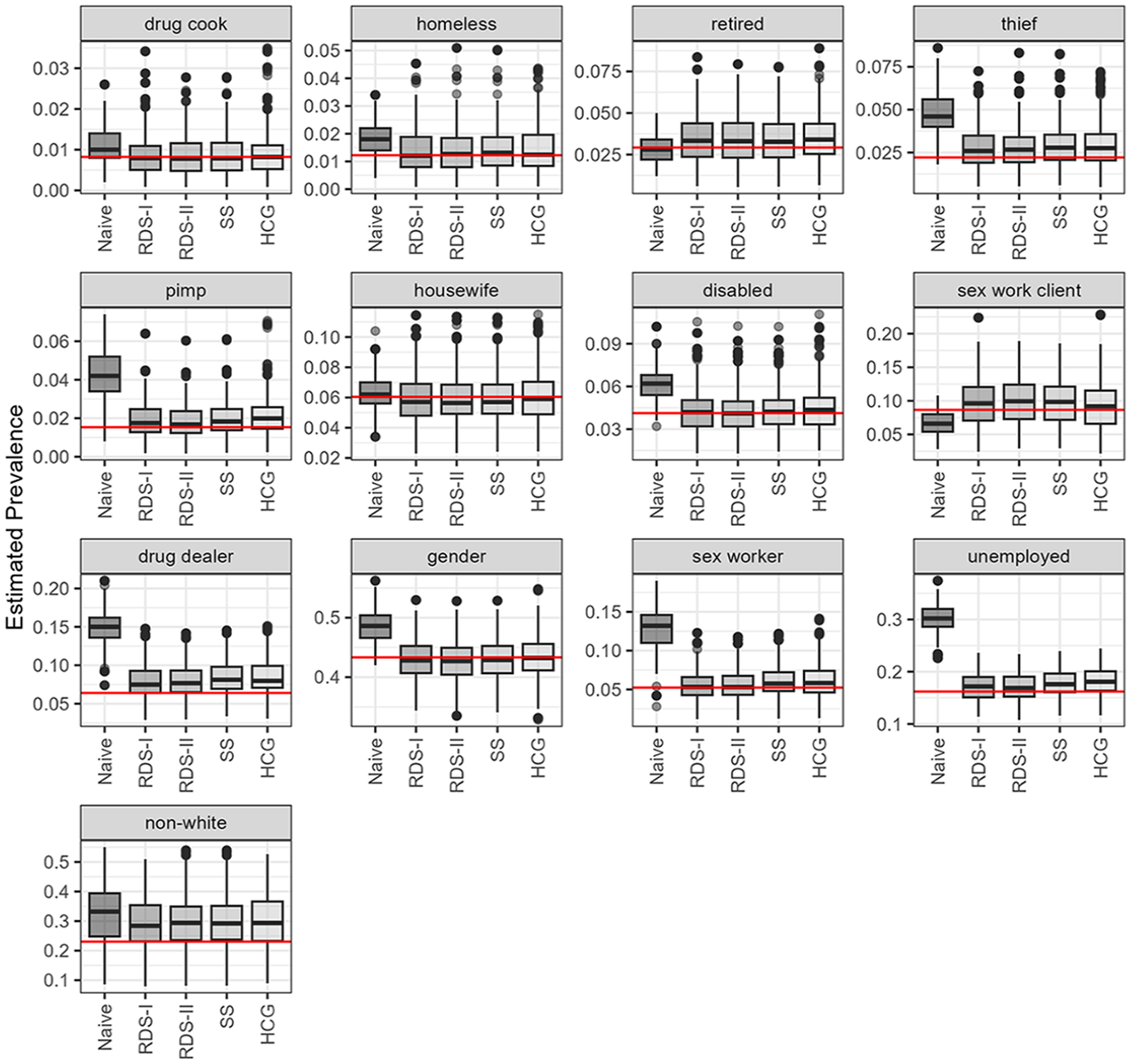
Estimates of trait prevalence for the Project 90 network across 1000 samples.

Table 2.

Coverage Rate, Root-Mean-Square Error, and Relative Bias of RDS Estimators for the Population Characteristics in the Project 90 Data Set

Status	Naive	RDS-I	RDS-II	SS	HCG
Coverage rate
Drug cook	.98	.77	.83	.83	.85
Homeless	.96	.66	.83	.83	.83
Retired	.91	.88	.93	.93	.91
Thief	.20	.49	.86	.84	.87
Pimp	.18	.44	.81	.76	.77
Housewife	.91	.80	.89	.88	.89
Disabled	.58	.67	.86	.86	.86
Sex work client	.52	.87	.91	.89	.84
Drug dealer	.00	.45	.85	.80	.78
Gender	.38	.86	.97	.97	.96
Sex worker	.02	.48	.92	.90	.91
Unemployed	.00	.75	.97	.95	.94
Non-White	.20	.31	.45	.43	.45
Root-mean-square error
Drug cook	.00	.01	.00	.00	.01
Homeless	.01	.01	.01	.01	.01
Retired	.01	.02	.02	.01	.02
Thief	.03	.01	.01	.01	.01
Pimp	.03	.01	.01	.01	.01
Housewife	.01	.02	.02	.02	.02
Disabled	.02	.01	.01	.01	.01
Sex work client	.03	.04	.04	.03	.04
Drug dealer	.09	.03	.03	.03	.03
Gender	.06	.03	.03	.03	.04
Sex worker	.08	.02	.02	.02	.02
Unemployed	.14	.03	.03	.03	.03
Non-White	.14	.11	.11	.11	.12
Bias
Drug cook	.29	.10	.04	.05	.09
Homeless	.49	.10	.11	.14	.15
Retired	−.04	.19	.18	.17	.20
Thief	1.17	.26	.27	.32	.32
Pimp	1.78	.24	.20	.29	.36
Housewife	.04	−.02	−.03	−.02	.00
Disabled	.49	.03	.01	.04	.06
Sex work client	−.22	.13	.15	.13	.08
Drug dealer	1.36	.24	.24	.31	.32
Gender	.12	−.01	−.02	−.01	.00
Sex worker	1.46	.06	.08	.16	.17
Unemployed	.86	.06	.06	.10	.12
Non-White	.40	.26	.27	.27	.29

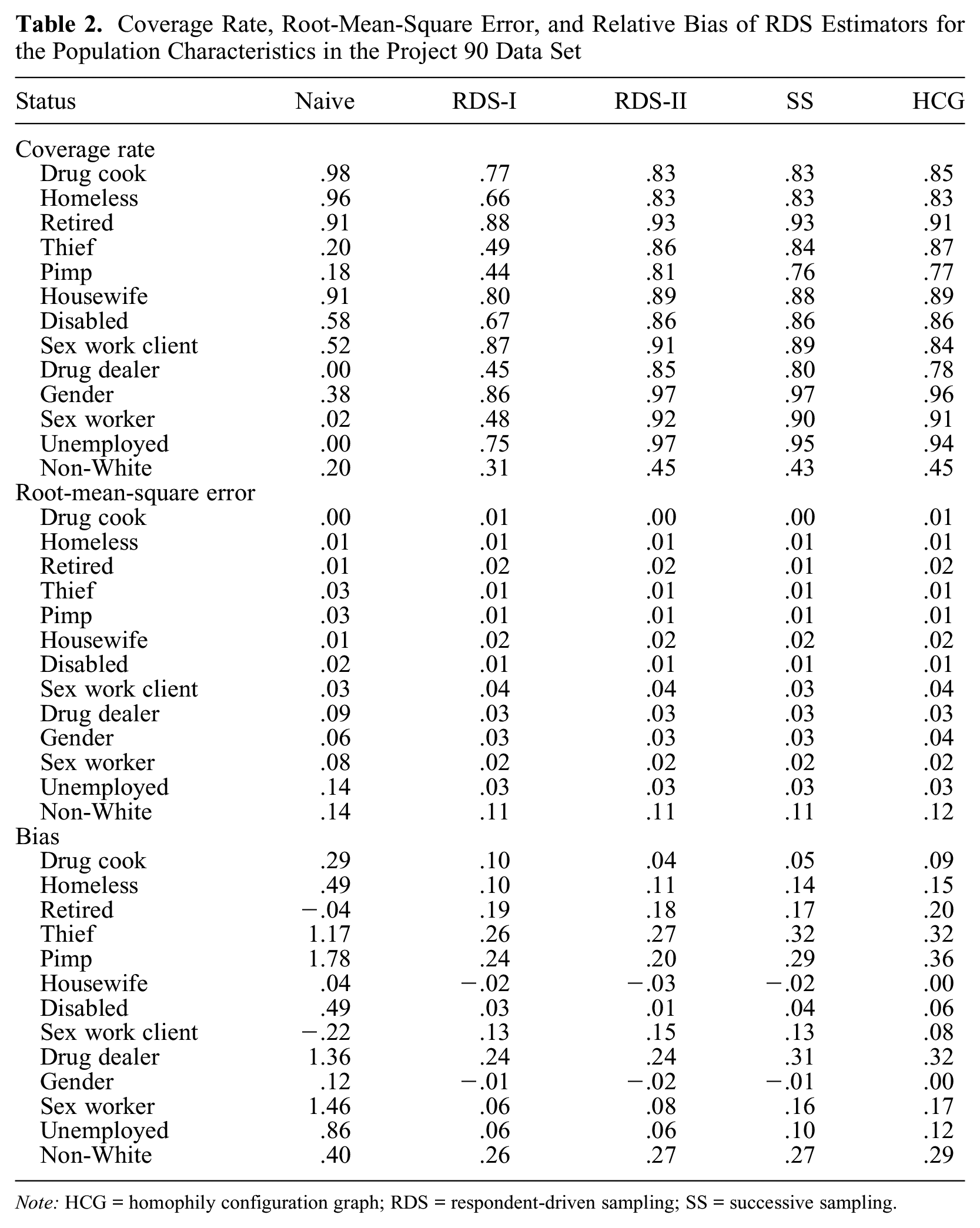
Note: HCG = homophily configuration graph; RDS = respondent-driven sampling; SS = successive sampling.

Simulated Categorical Outcomes and Large Facebook Pages Network

Figure S7 in the online supplement examines the performance of the estimators on the categorical outcomes from the Facebook Pages network and simulated populations. For the Facebook network, all categories exhibited similarly strong homophily, ranging from 5.3 to 5.7, but varied in their relative activity, which ranged from 0.40 to 2.46 (see the plot labels). The simulated networks were populations 6 and 11, with strong homophily, but this was moderated with the creation of the categorical outcomes. Traits a, b, and c had little homophily (1.0–1.8) for both populations, and only trait d had moderate homophily (i.e., 2.8 in the equal activity group and 2.6 in the elevated activity group). The RDS-I estimator produced many and extreme outliers, estimating prevalence of 1.0 or 0; in comparison, the modified RDS-I produced fewer outliers. The HCG estimator also produced large outliers, but never estimates of 0 or 1. The RDS-II and SS estimators performed similarly in all cases, as expected, because n << N. Coverage rates for all estimators are unacceptably low for categorical estimates (see Tables S8 and S9 in the online supplement).

Homophily and Relative Activity

For the simulated networks, we estimated the homophily and relative activity for each sample (see Figure S10 in the online supplement). On the basis of the large variability in the sample estimates, we strongly caution against drawing inferences about these population characteristics from RDS samples. The sample homophily estimates are unbiased for populations with no or moderate homophily, but they underestimate strong population homophily. Elevated activity at the population level was not detected by a simple ratio of the mean network degree between groups. Conversely, degree ratio on the basis of the Salganik-Heckathorn mean degree estimates overestimated relative activity. We found large variability in homophily and relative activity when trait prevalence was low. The difficulty in estimating population features from RDS samples provides impetus for identifying an estimator that performs well under varied conditions.

Discussion

We explored the properties of commonly used and reported RDS estimators in larger populations with degree distributions sampled from actual reported degree under conditions of equal and elevated relative activity and varying levels of homophily. We were able to achieve our target levels of prevalence and homophily and create populations with equal and elevated relative activity (Table 1) for networks with Poisson-distributed degree as well as from real-world reported degree samples. Note that neither homophily nor relative activity were precisely estimated from the RDS samples (see Figure S10 in the online supplement), and the level of precision depends on trait prevalence. Population relative activity is poorly estimated by the ratio of mean degree between groups. Because individuals with larger degree are more likely to be included in RDS samples (especially simulated ones), the overall degree of RDS samples is biased upward. Coupled with the log-normal degree distributions observed in real RDS samples, the mean degrees of both groups are higher in RDS samples than in the population, and their ratio tends to be biased toward 1. Thus, even when relative activity is present in the population, it is difficult to detect on the basis of sample information. As Figure S10 in the online supplement indicates, the estimate can be somewhat improved by using the inverse weighting employed by Salganik and Heckathorn (2004) in the RDS-I estimator, but substantial variability remains. The inability to assess network characteristics from RDS samples makes guidelines on estimator utility on the basis of these characteristics difficult in the absence of external knowledge about the target population.

Characteristics of the underlying population influence the accuracy of prevalence estimation from RDS samples. In particular, degree distribution affects the variance of RDS estimates (Figure 2) and must be considered when evaluating estimator validity. Previous RDS validation research has relied on degree distributions generated using ERGM or Poisson distributions, which have less variation than degrees reported by participants in real-world studies. A comprehensive survey of RDS samples showed that self-reported degree is log-normally distributed across a variety of population types (sex workers, men who have sex with men, people who inject drugs, migrants) and geographies (North America, India, Europe) (Avery et al. 2021). The degree distributions of the Project 90 and Large Facebook Pages networks (Figure S5 in the online supplement) indicate similar distributions. Thus, although our results are consistent with previous research with respect to the relative performance of the estimators, we report lower coverage rates and demonstrate increased variability, which we believe is more consistent with real-world performance. A Poisson-generated degree distribution resulted in coverage near nominal levels for the sample proportion and RDS-I estimator and near perfect coverage for the RDS-II, SS, and HCG (the latter two assuming that the population size was known exactly). When degree was sampled from real-world reported degrees, the coverage dropped considerably for all the RDS-specific estimators (Figure 2).

The naive sample proportion is a poor estimator for RDS samples. It has large bias when there is elevated activity in the group with the trait of interest, and it is especially poor (regardless of relative activity) when the prevalence is low. One then needs to decide which of the RDS-specific estimators to use. If relative activity between groups in the underlying population is equal, then the RDS-II estimator is preferred on the basis of low bias (common to all but the naive sample mean), low error, reasonable coverage, and no required knowledge of the population size (see Figures 3 and 4 and Tables S1–S4 in the online supplement). Note, though, that equal activity cannot be established from an RDS sample: the assumption of equal activity must be made using external knowledge of the target population. For example, it may be reasonable to assume that a hidden trait, such as blood type, would lead to groups with equal activity. The HCG and RDS-I estimators are biased, even under equal activity when homophily is strong. This was corrected with the modified RDS-I*, indicating that the bias is caused by extreme prevalence estimates resulting from no observed recruitments between groups in one direction. This supports use of the RDS-I estimator, because extreme prevalence estimates are easily identified.

We also recommend the RDS-II estimator when elevated activity is present. Despite a negative bias, the accuracy of the RDS-II is on par with the HCG estimator and importantly, the bias is consistent. In contrast, the bias of the HCG estimator depends on the direction of misspecification of the population size, with prevalence overestimated when population size is underestimated and vice versa. Finally, the coverage of the RDS-II estimator is comparable to the HCG, although reduced for elevated activity in combination with strong homophily. This can be partially rectified using the tree bootstrap (Table S1 in the online supplement). We evaluated the tree bootstrap confidence interval for sample sizes of 500, and it provides coverage near to the nominal rate unless strong homophily is present. The penalty for these accurate confidence intervals is uncertainty, with the width of confidence intervals greater than the trait prevalence, and nearly double the prevalence when strong homophily is present. For example, in a population with equal activity and no homophily, the coverage rate of the tree bootstrap for the RDS-II estimator was 0.97 for a trait prevalence of 0.2, with a median width of 0.22, indicating some confidence that the true prevalence is between 0.09 and 0.31. In contrast, the analytic estimator offers only 80 percent coverage, but the median width of the confidence interval is 0.04. The presence of strong network homophily increases the variability of all the estimators, naive and RDS specific. In this situation, too, the RDS-I estimator is more likely to fail and produce an extreme estimate of 0 or 1; this occurred in both simulated populations with strong homophily.

Similar to Gile (2011) and Fellows (2019), we found that the second-generation RDS estimators, Gile’s SS and the HCG, have improved accuracy and coverage relative to the earlier RDS-I and RDS-II estimators in the presence of elevated activity when the sample size is a substantial fraction of the population (in our study, n/N = 0.25). However, as Figures 3 and 4 indicate, the HCG and SS estimators are sensitive to misspecification of the population size in the presence of strong homophily. We varied $\hat{N}$ from N/2 to 10N (the imbalance was necessary because the sample size was N/4), and the interquartile range of HCG estimates was consistent with that of RDS-II. The bias of the HCG and SS estimators is related to the direction of the misspecification, and because the true population size is unknown, this introduces another layer of uncertainty in these estimates. It also raises the question of how a researcher with a single RDS sample would know if a substantial fraction of the population had been captured. The consistency of the RDS-II estimator may prove useful for surveillance studies in which the underlying population is dynamic and not easily estimated.

The Project 90 data support our simulation results, specifically that relative activity and strong homophily influence estimator performance. For the characteristics with elevated activity—gender, drug dealer, non-White, sex worker, and unemployed—the naive estimator overestimated prevalence substantially. Conversely, the naive estimator underestimated prevalence for the retired and sex work client traits, which exhibited reduced activity. The coverage rate, although often below the nominal level of 0.95, was greater than 0.75, except for the non-White characteristic. Among all the Project 90 characteristics, ethnicity displayed the greatest homophily, so the low coverage rate is unsurprising (Table 2). Our results contrast with Fellows (2019), in that the HCG was not the least biased estimator; instead, the RDS-I estimator performed well for this population and was similar to the RDS-II. The differences may be partly explained by the different populations used. Fellows restricted analysis to the single largest connected component of the population, whereas we drew from the entire population and modified the sampling process to include more seeds if recruitment stopped before the desired sample size was reached, to mimic real-world application of RDS.

The Large Facebook Pages network classified pages based on a categorical outcome: pages were classified as either company, TV show, politician, or government. There was moderate homophily (H ≅ 5) for each group, with varying relative activity. In this population, the RDS-II estimator was unbiased, as were the RDS-I and SS with the HCG displaying the greater bias, largest RMSE, and lowest coverage. The tree bootstrap on the modified RDS-I produced the best, but still lower than nominal coverage (Table S8 in the online supplement), again with very wide confidence intervals. To determine if the poor performance of the HCG estimator was specific to this network, we categorized our binary outcome for the populations with strong homophily, which had favored the HCG estimator, and we reexamined estimator performance. In both populations (with equal and elevated activity), the RDS-I and HCG had a large number of outlying estimates. We observed less variability in the modified RDS-I estimator (Figure S7 in the online supplement), indicating these outlying prevalence estimates are the result of not observing recruitment ties between some of the categories, which is more likely to occur the more categories there are. Therefore, our recommendation for categorical outcomes is clear: the RDS-II estimator should be used in all populations when the sample size is a small fraction of the population. Note that the absence of cross-group ties was observed even in these relatively large, simulated samples of n = 500.

Findings from the modified RDS-I* indicate that improvements to this estimator (and therefore the HCG) are possible. Further improvements to these estimators may reduce the variability observed when the trait prevalence is low. Low coverage is a problem that persists even with use of the tree bootstrap to calculate confidence intervals. Although the tree bootstrap does provide better coverage around the population prevalence, the large width of the confidence intervals, which range from double to quadruple other methods (Table S2 in the online supplement), limits the usefulness of this approach in practice.

A limitation of our study is the use of real-world reported network degree in our simulations. Because participants in RDS studies are sampled proportional to their connectivity, the mean degree of an RDS sample will be higher than the degree in the underlying population. However, the population-level degree distributions of the Large Facebook Pages network and the Project 90 network are similar to the reported degrees (see Figures S5 and S10 in the online supplement) and, even though these reported degrees may not be an accurate representation of population-level degrees, we believe this distribution more accurately reflects real-world networks than does the Poisson distribution. Further research could focus on the effect of mean population degree from log-normal distributions.

Despite additions to the RDS methodology toolkit, precise trait prevalence estimation remains elusive. Estimator performance depends on population characteristics that cannot be gleaned from RDS samples. The preferred estimator for each study should involve careful consideration of the most recent statistical literature and a well-informed understanding of both the population and the trait under study. Population homophily and relative activity will affect the choice of preferred estimator, and in the absence of good statistical estimates of these properties, good fieldwork is essential. If the goal is disease surveillance, the RDS-II should be considered because it has consistent bias, reasonable coverage, is independent of population size, and has good performance with categorical traits. Consistency is especially important in surveillance, in which accurately assessing change over time is the goal. Future evaluations of RDS estimators must incorporate real-world network data to capture the true variability in point estimates and accurately assess coverage rates.

Supplemental Material

sj-docx-1-smx-10.1177_00811750231163832 – Supplemental material for Evaluation of Respondent-Driven Sampling Prevalence Estimators Using Real-World Reported Network Degree

Supplemental material, sj-docx-1-smx-10.1177_00811750231163832 for Evaluation of Respondent-Driven Sampling Prevalence Estimators Using Real-World Reported Network Degree by Lisa Avery and Michael Rotondi in Sociological Methodology

Supplemental Material

sj-docx-10-smx-10.1177_00811750231163832 – Supplemental material for Evaluation of Respondent-Driven Sampling Prevalence Estimators Using Real-World Reported Network Degree

Supplemental material, sj-docx-10-smx-10.1177_00811750231163832 for Evaluation of Respondent-Driven Sampling Prevalence Estimators Using Real-World Reported Network Degree by Lisa Avery and Michael Rotondi in Sociological Methodology

Supplemental Material

sj-docx-2-smx-10.1177_00811750231163832 – Supplemental material for Evaluation of Respondent-Driven Sampling Prevalence Estimators Using Real-World Reported Network Degree

Supplemental material, sj-docx-2-smx-10.1177_00811750231163832 for Evaluation of Respondent-Driven Sampling Prevalence Estimators Using Real-World Reported Network Degree by Lisa Avery and Michael Rotondi in Sociological Methodology

Supplemental Material

sj-docx-3-smx-10.1177_00811750231163832 – Supplemental material for Evaluation of Respondent-Driven Sampling Prevalence Estimators Using Real-World Reported Network Degree

Supplemental material, sj-docx-3-smx-10.1177_00811750231163832 for Evaluation of Respondent-Driven Sampling Prevalence Estimators Using Real-World Reported Network Degree by Lisa Avery and Michael Rotondi in Sociological Methodology

Supplemental Material

sj-docx-4-smx-10.1177_00811750231163832 – Supplemental material for Evaluation of Respondent-Driven Sampling Prevalence Estimators Using Real-World Reported Network Degree

Supplemental material, sj-docx-4-smx-10.1177_00811750231163832 for Evaluation of Respondent-Driven Sampling Prevalence Estimators Using Real-World Reported Network Degree by Lisa Avery and Michael Rotondi in Sociological Methodology

Supplemental Material

sj-docx-5-smx-10.1177_00811750231163832 – Supplemental material for Evaluation of Respondent-Driven Sampling Prevalence Estimators Using Real-World Reported Network Degree

Supplemental material, sj-docx-5-smx-10.1177_00811750231163832 for Evaluation of Respondent-Driven Sampling Prevalence Estimators Using Real-World Reported Network Degree by Lisa Avery and Michael Rotondi in Sociological Methodology

Supplemental Material

sj-docx-6-smx-10.1177_00811750231163832 – Supplemental material for Evaluation of Respondent-Driven Sampling Prevalence Estimators Using Real-World Reported Network Degree

Supplemental material, sj-docx-6-smx-10.1177_00811750231163832 for Evaluation of Respondent-Driven Sampling Prevalence Estimators Using Real-World Reported Network Degree by Lisa Avery and Michael Rotondi in Sociological Methodology

Supplemental Material

sj-docx-7-smx-10.1177_00811750231163832 – Supplemental material for Evaluation of Respondent-Driven Sampling Prevalence Estimators Using Real-World Reported Network Degree

Supplemental material, sj-docx-7-smx-10.1177_00811750231163832 for Evaluation of Respondent-Driven Sampling Prevalence Estimators Using Real-World Reported Network Degree by Lisa Avery and Michael Rotondi in Sociological Methodology

Supplemental Material

sj-docx-8-smx-10.1177_00811750231163832 – Supplemental material for Evaluation of Respondent-Driven Sampling Prevalence Estimators Using Real-World Reported Network Degree

Supplemental material, sj-docx-8-smx-10.1177_00811750231163832 for Evaluation of Respondent-Driven Sampling Prevalence Estimators Using Real-World Reported Network Degree by Lisa Avery and Michael Rotondi in Sociological Methodology

Supplemental Material

sj-docx-9-smx-10.1177_00811750231163832 – Supplemental material for Evaluation of Respondent-Driven Sampling Prevalence Estimators Using Real-World Reported Network Degree

Supplemental material, sj-docx-9-smx-10.1177_00811750231163832 for Evaluation of Respondent-Driven Sampling Prevalence Estimators Using Real-World Reported Network Degree by Lisa Avery and Michael Rotondi in Sociological Methodology

Footnotes

Acknowledgements

We would like the thank our three reviewers, who offered insightful and constructive comments and have made a valuable contribution to the article.

Funding

The author(s) disclosed receipt of the following financial support for the research, authorship, and/or publication of this article: This research is supported by Canadian Institutes of Health Research grant 162468.

ORCID iD

Lisa Avery

Data Note

Simulated networked populations and code modification for RDS-I* are available on GitHub ().

Supplemental Material

Supplemental material for this article is available online.

Author Biographies

Lisa Avery is a principal biostatistician with University Health Network and an assistant professor of biostatistics at the Dalla Lana School of Public Health, University of Toronto. She has been practicing biostatistics for more than 20 years and has a wide variety of research interests, including outcome measurement, longitudinal modeling, RDS, and translational research.

Michael Rotondi is an associate professor of biostatistics at York University, Toronto, Canada, and holds a PhD in biostatistics from the University of Western Ontario, Canada. He has an extensive track record in both methodological and applied work in RDS and is funded by the Canadian Institutes of Health Research. Over the past 10 years, he has participated in a variety of RDS projects, including urban Indigenous communities in Canada, persons who inject drugs, and home care workers. His work has been published in various high-impact journals, including the Journal of Clinical Epidemiology, the Bulletin of the World Health Organization, Diabetes Care, and CMAJ.

References

Abdesselam

Kahina.

2019. “Network Distribution and Respondent-Driven Sampling (RDS) Inference about People Who Inject Drugs in Ottawa, Ontario.” PhD thesis, University of Ottawa, Ottawa, Canada.

Abdesselam

Kahina

Verdery

Ashton

Pelude

Linda

Dhami

Parminder

Momoli

Franco

Jolly

Ann M.

2020. “The Development of Respondent-Driven Sampling (RDS) Inference: A Systematic Review of the Population Mean and Variance Estimates.”Drug and Alcohol Dependence 206:107702.

Avery

Lisa

Macpherson

Alison

Flicker

Sarah

Rotondi

Michael

. 2021. “A Review of Reported Network Degree and Recruitment Characteristics in Respondent Driven Sampling Implications for Applied Researchers and Methodologists.”PLoS ONE 16(4):e0249074.

Baraff

Aaron J.

2016. “RDStreeboot: RDS Tree Bootstrap Method.” Retrieved March 17, 2023. https://CRAN.R-project.org/package=RDStreeboot.

Baraff

Aaron J.

McCormick

Tyler H.

Raftery

Adrian E.

2016. “Estimating Uncertainty in Respondent-Driven Sampling Using a Tree Bootstrap Method.”Proceedings of the National Academy of Sciences 113(51):14668–73.

Crawford

Forrest

. 2016. “The Graphical Structure of Respondent Driven Sampling.”Sociological Methodology 46(1):187–211.

Fellows

Ian E.

2019. “Respondent-Driven Sampling and the Homophily Configuration Graph.”Statistics in Medicine 38(1):131–50. https://onlinelibrary.wiley.com/doi/abs/10.1002/sim.7973.

Gile

Krista J.

2011. “Improved Inference for Respondent-Driven Sampling Data with Application to HIV Prevalence Estimation.”Journal of the American Statistical Association 106(493):135–46.

Gile

Krista J.

Beaudry

Isabelle S.

Handcock

Mark S.

Ott

Miles Q.

2018. “Methods for Inference from Respondent-Driven Sampling Data.”Annual Review of Statistics and Its Application 5:65–93.

10.

Goel

Sharad

Salganik

Matthew J.

2010. “Assessing Respondent-Driven Sampling.”Proceedings of the National Academy of Sciences 107(15):6743–47.

11.

Green

A.K.B.

McCormick

T. H.

Raftery

A. E.

2020. “Consistency for the Tree Bootstrap in Respondent-Driven Sampling.”Biometrika 107(2):497–504.

12.

Handcock

Mark S.

Gile

Krista J.

Fellows

Ian E.

Neely

W. Whipple

. 2021. “RDS: Respondent-Driven Sampling.” Retrieved March 17, 2023. http://wiki.stat.ucla.edu/hpmrg/.

13.

Handcock

Mark S.

Gile

Krista J.

Mar

Corinne M.

2014. “Estimating Hidden Population Size Using Respondent-Driven Sampling Data.”Electronic Journal of Statistics 8(1):1491–1521.

14.

Harris

Kathleen Mullan

Udry

J. Richard

. 2021. “National Longitudinal Study of Adolescent to Adult Health (Add Health), 1994–2018 [Public Use].”Chapel Hill: Carolina Population Center, University of North Carolina–Chapel Hill.

15.

Heckathorn

Douglas D.

1997. “Respondent-Driven Sampling: A New Approach to the Study of Hidden Populations.”Social Problems 44(2):174–99.

16.

Lachowsky

Nathan J.

Card

Kiffer G.

Cui

Zishan

Sereda

Paul

Roth

Eric A.

Hogg

Robert S.

Moore

David M.

2019. “Agreement between Gay, Bisexual and Other Men Who Have Sex with Men’s Period Prevalence and Event-Level Recall of Sexual Behaviour: An Observational Respondent-Driven Sampling Study.”Sexual Health 16(1):84–87.

17.

McCreesh

Nicky

Frost

Simon D. W.

Seeley

Janet

Katongole

Joseph

Tarsh

Matilda N.

Ndunguse

Richard

Jichi

Fatima

, et al. 2012. “Evaluation of Respondent-Driven Sampling.”Epidemiology 23(1):138–47.

18.

Potterat

John J.

Woodhouse

Donald E.

Muth

Stephen Q.

Rothenburg

Richard B.

Darrow

William W.

Klovdahl

Alden S.

Muth

John B.

2004. “Network Dynamism: History and Lessons of the Colorado Springs Study.” Pp. 87–114 in Network Epidemiology: A Handbook for Survey Design and Data Collection, edited by Morris

Oxford, UK: Oxford University Press.

19.

R Core Team. 2021. “R: A Language and Environment for Statistical Computing.” Vienna, Austria: R Foundation for Statistical Computing. Retrieved March 17, 2023. https://www.R-project.org.

20.

Rozemberczki

Benedek

Allen

Carl

Sarkar

Rik

. 2021. “Multi-scale Attributed Node Embedding.”Journal of Complex Networks 9(2):cnab014.

21.

Salganik

Matthew J.

Heckathorn

Douglas D.

2004. “Sampling and Estimation in Hidden Populations Using Respondent-Driven Sampling.”Sociological Methodology 34(1):193–240.

22.

Solomon

Sunil S.

Solomon

Suniti

McFall

Allison M.

Srikrishnan

Aylur K.

Anand

Santhanam

Verma

Vinita

Vasudevan

Canjeevaram K.

, et al. 2019. “Integrated HIV Testing, Prevention, and Treatment Intervention for Key Populations in India: A Cluster-Randomised Trial.”The Lancet HIV 6(5):e283–96.

23.

Spiller

Michael W.

Gile

Krista J.

Handcock

Mark S.

Mar

Corinne M.

Wejnert

Cyprian

. 2018. “Evaluating Variance Estimators for Respondent-Driven Sampling.”Journal of Survey Statistics and Methodology 6(1):23–45.

24.

Verdery

Ashton M.

Merli

M. Giovanna

Moody

James

Smith

Jeffrey A.

Fisher

Jacob C.

2015. “Respondent-Driven Sampling Estimators Under Real and Theoretical Recruitment Conditions of Female Sex Workers in China.”Epidemiology 26(5):661–65.

25.

Volz

Erik

Heckathorn

Douglas

. 2008. “Probability Based Estimation Theory for Respondent Driven Sampling.”Journal of Official Statistics 24(1):79–97.

26.

Weikum

Damian

Angela

Kelly-Hanku

Hou

Parker

Kupul

Martha

Amos-Kuma

Angelyne

Badman

Steven G.

Dala

Nick

, et al. 2019. “Kuantim Mi Tu (‘Count Me Too’): Using Multiple Methods to Estimate the Number of Female Sex Workers, Men Who Have Sex with Men, and Transgender Women in Papua New Guinea in 2016 and 2017.”JMIR Public Health and Surveillance 5(1):e11285.

27.

Wejnert

Cyprian

. 2009. “An Empirical Test of Respondent-Driven Sampling: Point Estimates, Variance, Degree Measures, and Out-of-Equilibrium Data.”Sociological Methodology 39(1):73–116.

Supplementary Material

Please find the following supplemental material available below.

For Open Access articles published under a Creative Commons License, all supplemental material carries the same license as the article it is associated with.

For non-Open Access articles published, all supplemental material carries a non-exclusive license, and permission requests for re-use of supplemental material or any part of supplemental material shall be sent directly to the copyright owner as specified in the copyright notice associated with the article.

0.00 MB

0.02 MB

0.01 MB

0.39 MB

0.01 MB

0.02 MB

0.19 MB

0.03 MB

0.02 MB