
Abstract
In this article, a modeling strategy is proposed that accounts for heterogeneity in nominal responses that is typically ignored when using common multinomial logit models. Heterogeneity can arise from unobserved variance heterogeneity, but it may also represent uncertainty in choosing from alternatives or, more generally, result from varying coefficients determined by effect modifiers. It is demonstrated that the bias in parameter estimation in multinomial logit models can be substantial if heterogeneity is present but ignored. The modeling strategy avoids biased estimates and allows researchers to investigate which variables determine uncertainty in choice behavior. Several applications demonstrate the usefulness of the model.
Keywords
Introduction
The modeling of heterogeneity in binary and ordinal response models has been a topic of intensive research. In particular, Allison’s (1999) demonstration that comparisons of binary model coefficients across groups can be misleading if one has underlying heterogeneity of residual variances has stimulated research in the area. Williams (2009), Mood (2010), Rohwer (2015), Karlson, Holm, and Breen (2012), and Breen, Holm, and Karlson (2014) have all investigated ways to deal with this problem.
One approach is based on the heterogeneous choice model, in which an explicit term is included that accounts for variance heterogeneity (see Williams 2009, 2010). McCullagh (1980) considered an earlier version of the model under the name location-scale model, but the importance of modeling variance heterogeneity was not recognized until much later. Tutz and Berger (2016, 2017) proposed alternative models to account for variance heterogeneity in ordinal models. The considered location-shift models use an additive parameterization unlike the heterogeneous choice model, which uses a multiplicative predictor. Nevertheless, location-scale and location-shift models typically show similar goodness of fit. However, both models assume the response is ordinal.
CUB-type mixture models (i.e., combination of discrete uniform and binomial distribution) account for heterogeneity in ordinal responses. These models assume the observed response results from a mixture of an ordinal response model and an uncertainty component. The latter is determined by a uniform discrete distribution over categories. It is assumed to represent respondents’ uncertainty. Explanatory variables can determine the probabilities of the mixture. D’Elia and Piccolo (2005), Iannario and Piccolo (2010), Iannario (2012), Tutz et al. (2017), and Iannario et al. (2020) all considered models of this type, and Piccolo and Simone (2019) provided an extensive overview.
It is surprising that prior work has considered heterogeneity only for ordinal responses, not for unordered responses. In many surveys (e.g., surveys that cover party preference), respondents are asked to choose from a set of categories that represent distinct but not ordered alternatives. In the special case of binary choices, the heterogeneous model applies but CUB-type models fail because they work only for more than two categories. However, for more than two response categories, both types of model explicitly assume that categories are ordered.
Here, we consider the case of unordered response categories, in which response categories are mere labels without any inherent ordering. Social scientists use choice models for this type of response when modeling party preference, for example, or the choice of brands in economic applications. In such cases, respondents choose from a set of
A model is proposed that accounts for additional heterogeneity not captured by the linear parametric terms in the MLM. Heterogeneity is modeled as a function of explanatory variables that modifies the response probabilities. Heterogeneity can be interpreted as variance heterogeneity but also as respondents’ uncertainty. The resulting model is a truly multicategorical model, which, in contrast to the classical MLM, cannot be estimated by considering subsets of two response categories. The main benefits of the modeling strategy are that (1) the approach accounts for potential heterogeneity in unordered choices; (2) we avoid bias in parameter estimates, which can be substantial if heterogeneity is present but ignored; and (3) we obtain information on the dependence of choice uncertainty on explanatory variables.
The Heterogeneous MLM
Let

where for simplicity
Accounting for Heterogeneity
Let

For any two categories, we thus have

The predictors in the model comprise two components: the location terms,
For
For
With varying parameter
If
If we use the first category as a reference category by setting

where
Interpretation of Parameters and Motivations of the Model
The effect of the scaling component has not always been presented clearly in the classical heterogeneous model; in particular, it is often interpreted solely as representing variances. Therefore, we consider in the following several ways to interpret effects.
Variance Heterogeneity and Random Utilities
One way to motivate the multinomial model is to consider it as a random utility model. Let

Thus, we choose the alternative that maximizes the random utility. If we assume that

(e.g., McFadden 1973; Yellott 1977). By setting
Let us now assume, more generally, that the random utilities are given by

where again
The derivation suggests the modification of effect strength
Note that a scaling problem might affect the interpretation of parameters even when variances do not explicitly depend on covariates. Parameters in the model are then given by
Uncertainty
In questionnaires in which respondents choose among unordered alternatives, heterogeneity in variances of underlying utilities can be seen as uncertainty. If the variance is large, the preference for specific categories becomes less distinct; if variance is small, the category with the largest value in the location term
However, the scaling term
Varying Coefficients and Interactions
More generally, the model can also be seen within the framework of varying coefficients, proposed by Hastie and Tibshirani (1993) and extended by Cai, Fan, and Li (2000), Antoniadis, Gijbels, and Verhasselt (2012), and Park et al. (2015). For simplicity, let the scaling component contain the single binary variable

where

which means the proportion between the interaction effect
From a slightly different viewpoint, interactions can be seen as varying coefficients. Varying-coefficient models allow one to model effects that are modified by other variables. An advantage is that no reference to latent motivating variables is needed. These models aim to identify which effects are not stable across the variation of other variables and provide a general concept for interpretation of effects in models that account for the type of heterogeneity considered here. For the binary response case, Tutz (2020) investigated varying coefficients and the simpler form of constraints.
The representation as a model with interactions holds also in the case where
Measurement of Variability in Nominal Responses
Let us comment briefly on the general problem of measuring variability in a nominal response. Because the variable
This is in line with the effect of the heterogeneity term in the HMLM, in which the probabilities are determined by covariates. Because the probabilities depend on covariates, concentration is different for persons with different explanatory variables. Thus, the category-specific location terms, which are present in the simple and the extended nominal logit model, already generate heterogeneous concentration. The heterogeneity term, which is not category specific, modifies this basic structure, yielding stronger concentration if
In summary, whatever the interpretation of
Note that heterogeneity in the model is linked to covariates. It is not modeled on the individual’s level in the form of random effects, which might be interesting but hard to obtain without repeated measurements. It is a population-averaged approach, in contrast to conditional modeling approaches that consider responses given covariates and subject-specific parameters (for the distinction between conditional and population-averaged approaches, see, e.g., Neuhaus, Kalbfleisch, and Hauck 1991).
Identifiability
Identifiability of the parameters in a model is critical, because only then is reliable inference on parameters possible. Parameters of the heterogeneous multinomial model are identifiable if
However, parameters are identified if the number of predictors in
Nevertheless, one also wants to allow for a vector of explanatory variables in the heterogeneity terms, although it will be typically shorter than the vector of variables in the location term. In the Appendix, it is shown that, in general, the parameters of the heterogeneous model are identifiable if
Ignoring Heterogeneity
To demonstrate that parameter estimates can be severely biased if heterogeneity is ignored, we show some results of a simulation study. We include two explanatory variables, one binary, following a Bernoulli variable
Figure 1 shows estimates of
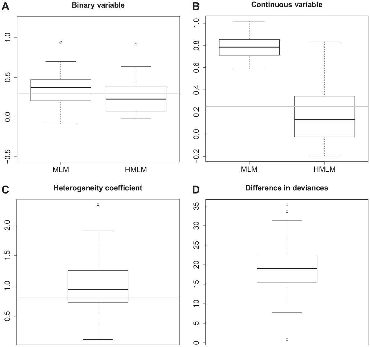
Estimates of parameters in simulation study with heterogeneity in continuous variable.
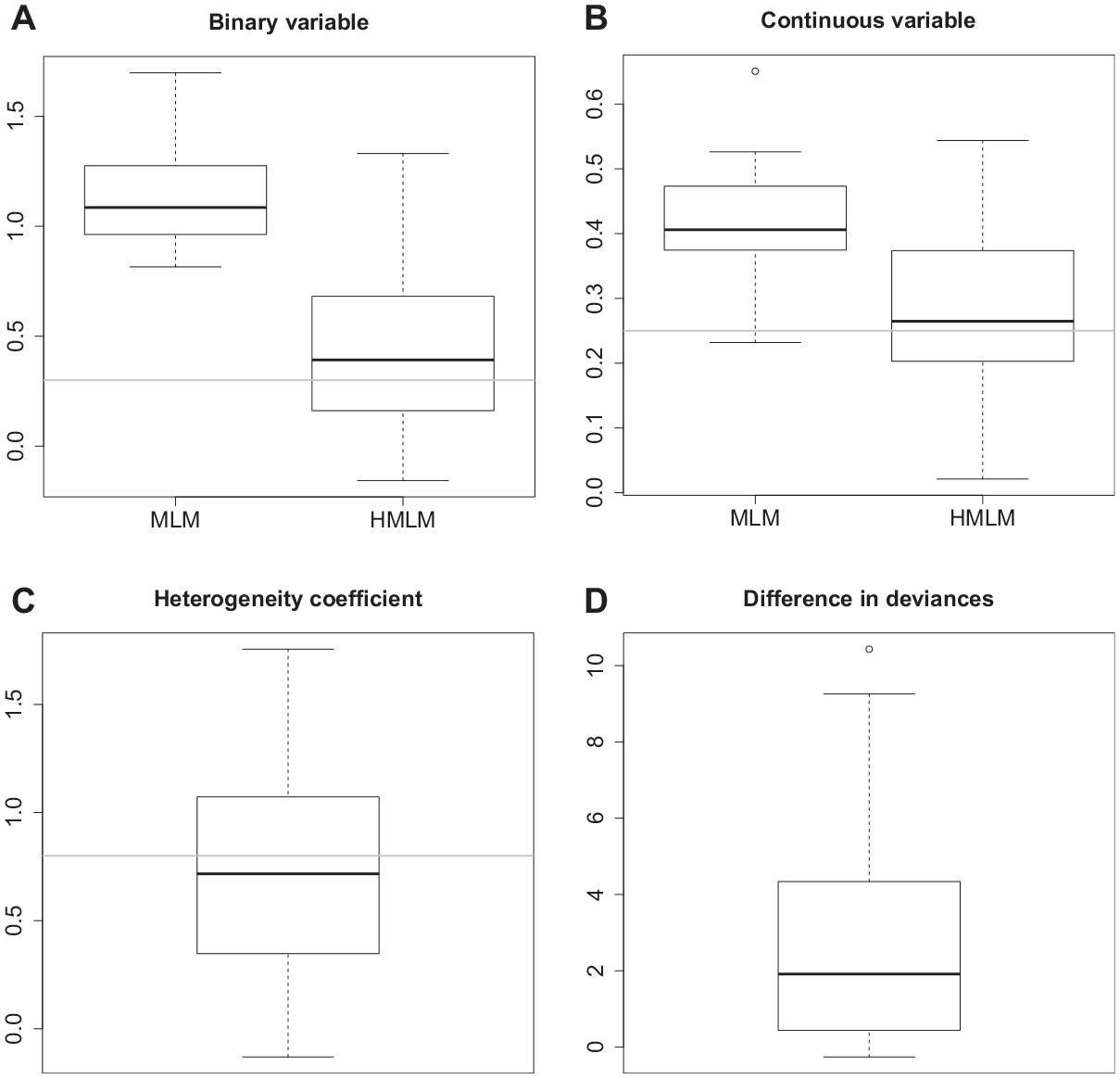
Estimates of parameters in simulation study with heterogeneity in categorical variable.
The effect of varying values of
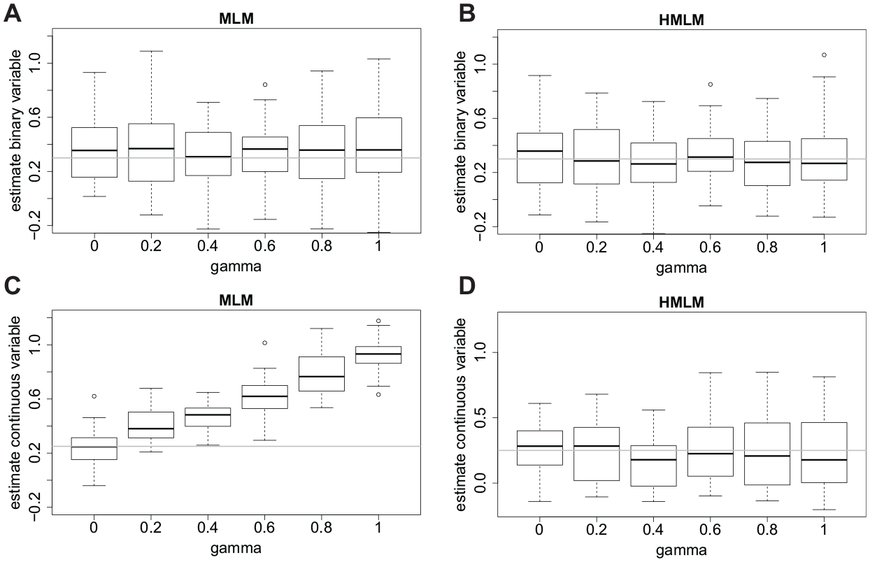
Estimates of parameters for varying
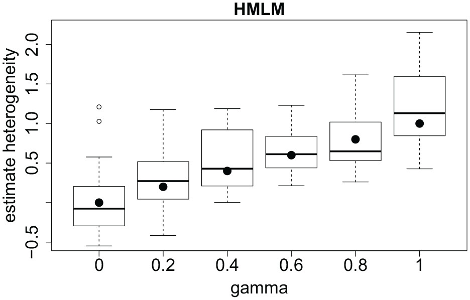
Estimates of heterogeneity parameter for varying
Modeling with Heterogeneity
The following sections demonstrate the usefulness of the modeling approach in several applications. The Appendix provides details on how to obtain the estimates.
Party Choice
We consider modeling of party choice with data from the German Longitudinal Election Study. The data are included in the R package EffectStars (Schauberger 2019). The response categories refer to the dominant parties in Germany: the Christian Democratic Union (CDU; category 1), the Social Democratic Party (SPD; category 2), the Liberal Party (FDP; category 3), the Green Party (category 4), and the Left Party (Die Linke; category 5). The explanatory variables are age (standardized), gender (1 = male, 0 = female), and regional provenance (west; 1 = former West Germany, 0 = otherwise). The sample size is
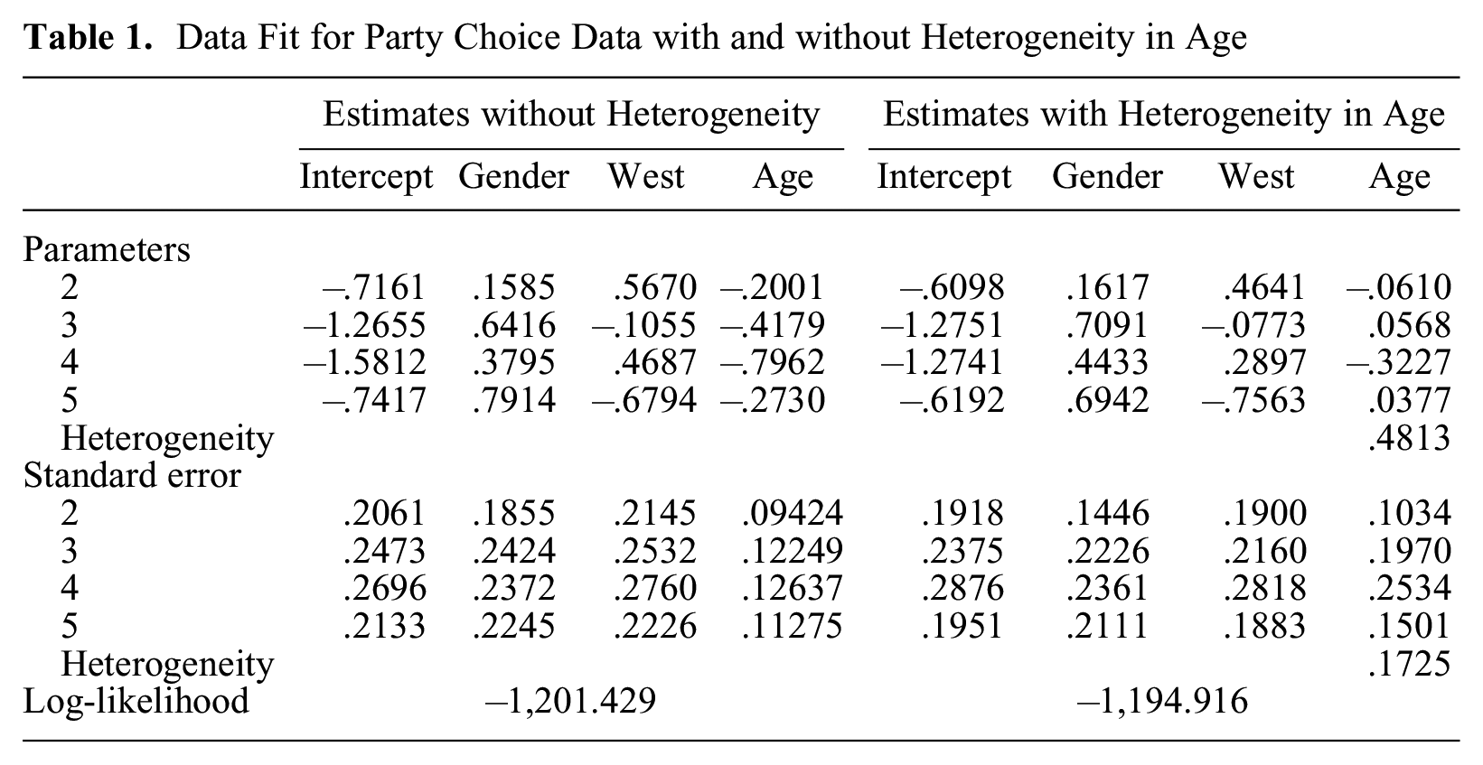
For illustration, let us first investigate if age is an effect-varying variable. Table 1 shows parameter estimates of the MLM and HMLM models with age in the scaling component. We see that the heterogeneity effect of age should not be neglected (value = .481, s.e. = .172). Older respondents show more distinct preferences for political parties than do younger respondents. The parameters obtained for the heterogeneity model differ from the parameters obtained without accounting for heterogeneity. In particular, the age parameters are much closer to zero for the heterogeneity model. However, that does not mean age has a weaker effect on the response. Figure 5 shows the effect of age for males living in the western part of the country. The dotted lines show the effects on probabilities in the multinomial model without heterogeneity; the gray lines represent the effects in the heterogeneous model. The change of probabilities across age is modified, but the effect of age has a very similar tendency. The high significance of the heterogeneity effect suggests part of this effect might be due to heterogeneity.
Data Fit for Party Choice Data with and without Heterogeneity in Age
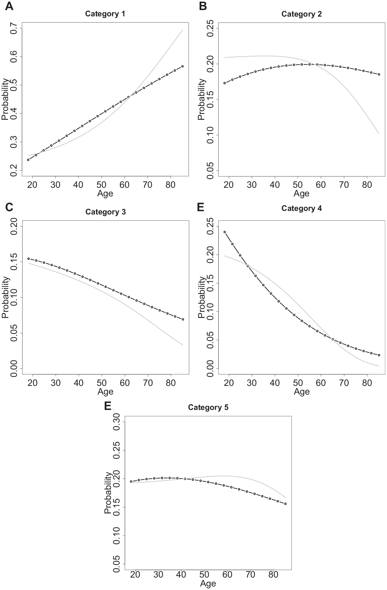
Effects of age on probabilities with age as heterogeneity variable for party choice data.
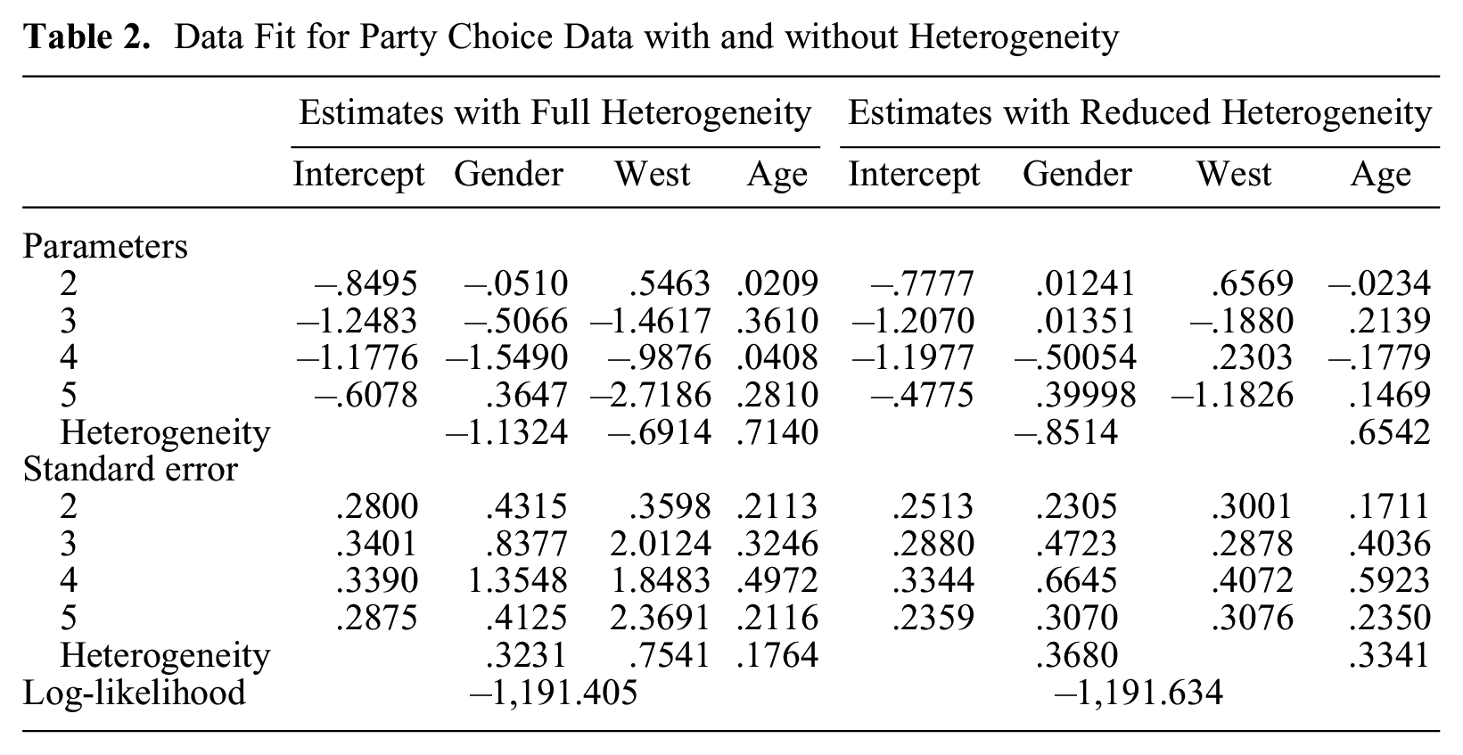
Age is not the only variable that might modify effect strengths. Including one variable at a time shows the variable gender is significant, but not the variable west. Table 2 (right-hand columns) shows parameter estimates of the HMLM model with heterogeneity effects of gender and age. We see that they should not be neglected and included simultaneously. We also fitted a model that includes all variables in the scaling component (left-hand columns). The fit also shows the heterogeneity effect of gender and age should not be neglected. Modification of the age effect is rather similar to that seen in Figure 5 and is not shown.
Data Fit for Party Choice Data with and without Heterogeneity
Contraceptive Prevalence Survey
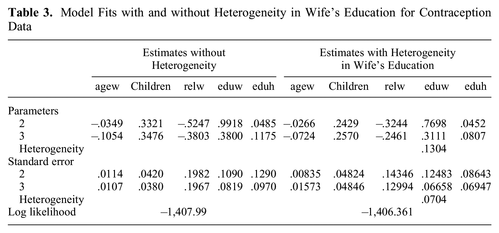
This dataset is a subset of the 1987 National Indonesia Contraceptive Prevalence Survey, available from the UCI Machine Learning Repository (Contraceptive Method Choice Data Set). The samples are married women who were either not pregnant or did not know if they were pregnant at the time of interview. The response is the contraceptive method used (1 = no use, 2 = long-term use, 3 = short-term use). The explanatory variables are wife’s age in years (agew), wife’s education (eduw; 1 = low, 2, 3, 4 = high), husband’s education (eduh; 1 = low, 2, 3, 4 = high), number of children ever born (children), and wife’s religion (relw; 0 = non-Islam, 1 = Islam). The sample size is n = 1,473. Fitting models shows that for most variables, there is no heterogeneity effect. The exception is wife’s education. Table 3 shows the models without and with heterogeneity in that variable. The effect strengths of variables is much weaker if we account for heterogeneity in wife’s education. For example, the effects of children are .33 and .34 if the MLM is fitted but .24 and .25 if the HMLM is fitted. The effects of variables might be overestimated if heterogeneity is ignored.
Model Fits with and without Heterogeneity in Wife’s Education for Contraception Data
Satisfaction Data
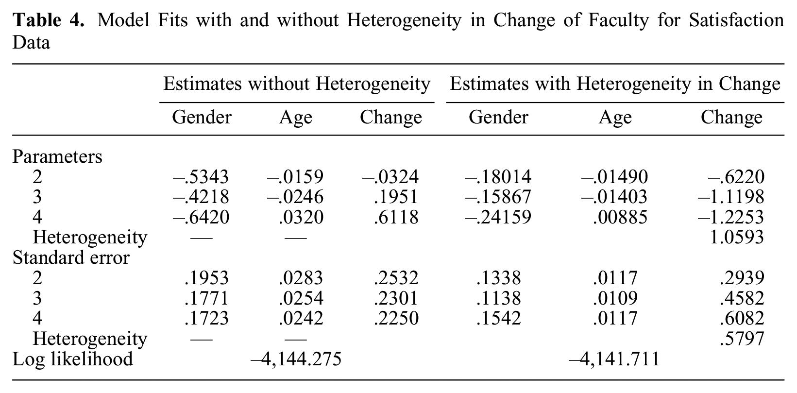
The data contain students’ satisfaction with the faculty at Universita degli Studi di Napoli Federico II, available in the R package CUB (data set CUBevaluation2008). Response categories are level of global satisfaction: 1 = neutral, 2 = not satisfied, 3 = satisfied, and 4 = very satisfied, which is only partially ordered. Explanatory variables are gender (0 = male, 1 = female), age in years, and change of faculty (1 = changed faculty, 0 = did not change faculty). Sample size is n = 4,042. Change was the only variable to show significant heterogeneity, which seems sensible as students who change faculty should be less certain about the new faculty. Table 4 shows the fits of the model without and with heterogeneity in the variable change. We again see that the effect of variables might be overestimated if heterogeneity is ignored. For example, the effects of gender are –.53, –.42, and –.64 if the MLM is fitted but merely –.18, –.15, and –.24 if the HTML is fitted.
Model Fits with and without Heterogeneity in Change of Faculty for Satisfaction Data
Further Issues
We now briefly consider marginal modeling and how models behave when applied to subsets of response categories. It is also investigated how the heterogeneous model can be used to deal with the problem of irrelevant alternatives. In a change of perspective, I emphasize that subsets of response categories refer to differing populations.
Marginal Effects and Modeling Strategies
One approach to circumvent identifiability problems uses the predicted probability metric to investigate marginal effects of predictors. Long and Mustillo (2018) show how this approach can be used to compare groups in binary regression models. With
Using probabilities instead of focusing on coefficients is helpful if one wants to compare specific groups, but it is less appropriate as a general modeling strategy that includes potential heterogeneity. Avoiding investigating coefficients is an advantage, but this approach has some limitations. In particular, the focus is on comparison of groups, not investigating general marginal effects. In addition, the comparisons work under the assumption that the variables that are not currently investigated are held fixed at specific values. This means conditional effects are investigated, not marginal effects in the sense of collapsing over the other variables. As Agresti and Tarantola (2018) noted, the “marginal effect” terminology is a bit misleading but seems to be in common use. Because the effects are conditional, the conclusions depend on the specific chosen values of the other variables, and it is harder to do when some of these variables are continuous. One also must select what sort of change, discrete or average, one wants to investigate.
A crucial difference with models that explicitly specify heterogeneity components is that marginal approaches use classical regression models with interactions. The model
The curves in Figure 5 show the effect of explanatory variables on the probabilities, which is a main objective of marginal approaches. This allows researchers to test if groups differ in terms of predicted probabilities. Within the heterogeneity model approach, the effect on probabilities is an effect of parameters. A variable such as age has an effect if it cannot be neglected in the location or the heterogeneity term, which can be tested. Then, the effect on probabilities is tested indirectly, but not directly as in marginal approaches. The advantage is that one does not have to condition on specific values of the other variables; the downside is that one does not use the natural marginal effect metric, which uses the probabilities. But as in binary response cases, one can compare groups regarding their marginal effects by using the predicted probabilities, as proposed by Long and Mustillo (2018) (see the Appendix for details). Simple ways to interpret effects of explanatory variables using the marginal metric may also be obtained by deriving generalizations of descriptive measures (see Agresti and Tarantola 2018).
One advantage of pure location models as used in the marginal approach is that estimates are easier to obtain than in multiplicative models. Keele and Park (2006) demonstrated this for the binary heteroskedastic model and showed that larger sample sizes are needed to obtain reliable estimates in heterogeneity models. Also, misspecification might have a stronger effect in heterogeneity models than in simple location models. This means care is needed when selecting variables in the location and the heterogeneity term. In some applications, one might suspect heterogeneity in specific variables for substantive reasons, and investigate if this suspicion is warranted. If there are no clear candidates but one wants to account for possible heterogeneity, one must select the variables that actually contribute to improve the fit. It seems sensible to include variables in the heterogeneity term only if they have strong effects that should not be neglected. If effects are weak, models that ignore heterogeneity might be preferable. Keele and Park even argued that in some cases it might be better to estimate standard models. However, the choice certainly depends on the strengths of the effects and therefore on the concrete application.
The location term is less critical, but it can be useful to include interaction effects, which might affect the relevance of variables in the heterogeneity term. In general, model choice and therefore variable selection is harder than in classical models, because one has two terms in which variables can be present, and because of the multiplicative structure. Even in classical regression models, stepwise selection procedures have some disadvantages and have been widely replaced by selection tools that are based on penalization as the lasso and its various extensions (Tibshirani 1996; Yuan and Lin 2006; Zhao, Rocha, and Yu 2009). In future research, similar methods could be used to address selection problems in heterogeneity models using differing penalties for inclusion in the location and the heterogeneity term, but methods for this advanced form of variable selection are not yet available even for the simpler binary heteroscedastic model.
Effect Modifiers and Independence from Irrelevant Alternatives
The MLM has a property typically referred to as independence from irrelevant alternatives, which has been called a blessing and a curse (McFadden 1986). It may be seen as a blessing because if it holds, it makes it possible to infer choice behavior with multiple alternatives using data from simple experiments like paired comparisons. Yet it is a rather strict assumption that may not hold for heterogeneous patterns of similarities among alternatives. In the following, we consider how this property can be addressed by allowing for the presence of effect modifiers.
Subsets of Response Categories and the Red Bus–Blue Bus Problem
If the logit model holds, we obtain for a subset of response categories

which is a logit model with response categories

which means

This is a counterintuitive result because the additional “irrelevant” blue bus substantially decreases the choice probability of driving. Similar problems hold for all choice systems that share a property called simple scalability (see Hausman and Wise 1978; Tversky 1972).
The Presence of Effect Modifiers
The independence of irrelevant alternatives raises problems if one wants to combine results from different choice sets and one assumes the multinomial model holds. These problems can be avoided when using the heterogeneous logit model if we assume the choice is an effect modifier. We now demonstrate this for the red bus–blue bus problem.
Let us assume the heterogeneous logit model holds with predictor

and


With


which are sensible values if one chooses from the three alternatives. For binary choices, we have

because

Thus, if we allow
Prior approaches to address the problem of similar alternatives in the choice set use more general distributions in the underlying latent trait model. In particular, the nested logit model and more general models based on the generalized extreme-value distribution have been developed (McFadden 1978, 1981). These models are derived from underlying random utilities but have the disadvantage that one must specify beforehand which alternatives are to be considered similar; they are used mainly in transportation research (see, e.g., Cai et al. 2000; Wen and Koppelman 2001) and less to analyze questionnaire data in the social sciences. Olsen (1982) proposed an alternative approach to address the problem.
The Heterogeneous Logit Model in Subpopulations
The red bus–blue bus problem arises if people must choose from different subsets of alternatives. The question is what can be inferred from the choice of categories if a different set of categories has been presented earlier. In the previous section, it was shown that it might be sensible to include the choice set in the predictors as heterogeneity components.
Subsets of categories can also be seen from a different view: the problem is not the transfer to other presented categories, but if models and parameters are the same given that one fits models to varying subsets. If the heterogeneous logit model holds for
Let us consider the party choice data, in which there were five parties—the CDU (category 1), the SPD (category 2), the FDP (category 3), the Green Party (category 4), and the Left Party (category 5)—and we found heterogeneity for the variables west and age. If we fit the model in a reduced set, say the first three parties, we have a different population, because we exclude everyone who tends to strongly favor left-wing parties or is strongly interested in ecological issues. Thus heterogeneity might differ.
We briefly consider the variation in estimates for the party data set. Table 5 shows estimates of the heterogeneity parameters for the variables west and age for varying sets of response categories. They are given in the exponential form
Heterogeneity in Variables West and Age for Varying Response Categories in Party Choice Data
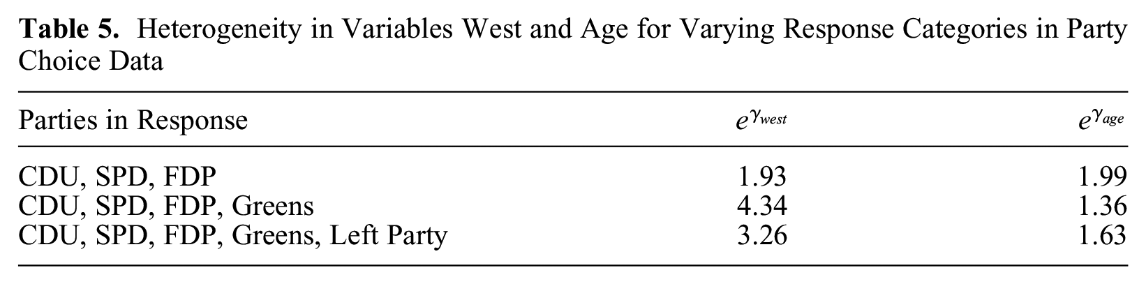
Although there is some variation in estimates, the tendency is the same in all subpopulations: people living in western Germany have a stronger tendency to specific categories than do people from the East, and the same holds for older versus younger respondents. Heterogeneity for the variable age is comparatively stable across subsets, but there is some variation in heterogeneity linked to the variable west.
Concluding Remarks
The proposed heterogeneous logit model is able to account for heterogeneity that is typically ignored in MLMs. This heterogeneity can be seen as unobserved variance heterogeneity but also as representing uncertainty without reference to latent variables. The model contains multiplicative terms, which are typically harder to estimate than simple linear terms and show greater variability. Models of this type have been criticized in the binary case because they are less stable than simple binary logit models (Kuha and Mills 2017). However, this is to be expected. Estimation of variance is usually harder to do than estimation of location. The alternative, ignoring heterogeneity, yields stable estimates, but they can be severely biased. Therefore, it seems worthwhile to account for potential heterogeneity.
Nevertheless, stable estimation of variance components typically calls for larger data sets. In small data sets, they are hard to identify and estimate. Fortunately, they often turn out to be negligible and can be ignored. For example, in a data set that contains high school students’ choices among general, vocational, or academic programs from the UCLA Statistical Consulting site (
In principle, one could allow for category-specific heterogeneity terms letting uncertainty depend on alternatives. One disadvantage is that one loses the derivation from the random utilities. More seriously, the number of parameters would be much higher and stability of estimates would suffer. Therefore, we abstained from considering the more general model with alternative dependent heterogeneity terms.
In the applications, an R program was used. The code for fitting the models will be made available on GitHub (GerhardTutz/GHMNL).