
Abstract
The dynamics of individual behavior are related to the dynamics of the social structures in which individuals are embedded. This implies that in order to study social mechanisms such as social selection or peer influence, we need to model the evolution of social networks and the attributes of network actors as interdependent processes. The stochastic actor-oriented model is a statistical approach to study network-attribute coevolution based on longitudinal data. In its standard specification, the coevolving actor attributes are assumed to be measured on an ordinal categorical scale. Continuous variables first need to be discretized to fit into such a modeling framework. This article presents an extension of the stochastic actor-oriented model that does away with this restriction by using a stochastic differential equation to model the evolution of a continuous attribute. We propose a measure for explained variance and give an interpretation of parameter sizes. The proposed method is illustrated by a study of the relationship between friendship, alcohol consumption, and self-esteem among adolescents.
1. Introduction
Social actors, such as people, organizations, and countries, simultaneously shape and are shaped by their social context. For example, individuals may select their friends based on their behavior, but they may also change their own behavior based on that of their friends. Social relationships among actors, such as friendship or collaboration, can be represented in social networks. These networks can change over time, often in interdependent relation with changing actor characteristics. While earlier studies of network dynamics were mainly descriptive in nature, many statistical models for network dynamics have been developed since (e.g., Almquist and Butts 2014; Doreian and Stokman 1997; Krivitsky and Handcock 2014; Robins and Pattison 2001; Snijders 2001, 2005). For the study of the interdependent dynamics of networks and individual behavior, the stochastic actor-oriented model is widely used (Snijders, Steglich, and Schweinberger 2007; Steglich, Snijders, and Pearson 2010).
The stochastic actor-oriented model can be used to test hypotheses about the social mechanisms driving network and actor attribute dynamics and study the interdependent processes of partner selection and social influence. One basic assumption of the model proposed by Snijders et al. (2007) is that dynamic actor attributes are measured on an ordinal scale with a limited number of categories. Under this assumption, the network and attribute evolution can be represented in a common statistical framework (i.e., by a continuous-time Markov chain with a discrete outcome space). However, restricting the coevolving attribute to a limited number of categories has proven to be a practical limitation in several studies because of the necessity to discretize attributes measured on a very fine-grained or continuous scale.
In a study of the development of body weight of adolescents and their friendships, for example, Haye et al. (2011) split the dependent attribute, body mass index, into ordered categories to make their analysis feasible. Flashman (2012) measured scholastic achievement on a continuous scale and later transformed it into a five-point scale for the same purpose. Some other continuous variables that had to be treated similarly are job satisfaction (Agneessens and Wittek 2008), self-reported and peer-reported aggression and victimization (Dijkstra et al. 2012), and physical activity (Gesell, Tesdahl, and Ruchman 2012).
For corporate actors, performance indicators composed of multiple variables and monetary outcomes are often measured on a continuous scale. Many individual physical attributes are continuous variables. Psychological scales often assume the existence of one or more latent continuous dimensions, measured on a fine-grained categorical scale. For all such measures, discretization into a few categories would involve arbitrary choices (number and width of categories) and could lead to loss of information. Moreover, different discretizations could lead to different results.
The role of peers for organizational performance or individual health outcomes has been the subject of several studies (e.g., Checkley et al. 2014; Haye et al. 2011). Psychological characteristics may be susceptible to social influence (e.g., depression through corumination), but they may also play a buffering role. People with certain psychological characteristics might be more susceptible to influence by their peers than others. If we want to study such a moderating effect, unless the characteristic is a stable personality trait, we need to model the network through which influence occurs, the variable that is influenced, and the psychological moderator as three coevolving elements.
Motivated by the practical limitations discussed previously, Niezink and Snijders (2017) have extended the stochastic actor-oriented model for the coevolution of networks and continuous actor behavior. In this article, we first give an applied introduction to this model. Newly treated in the current study are a proposal for defining explained variance and an extensive discussion about interpretation of results, two topics that are not addressed in Niezink and Snijders (2017) but that are essential for the model to be useful in practice. We use the method to study whether self-esteem moderates adolescents’ susceptibility to peer influence on alcohol use by combining a stochastic actor-oriented model for the coevolution of a network and a discrete individual behavior variable (Steglich et al. 2010) with the model for continuous actor behavior (Niezink and Snijders 2017). The study illustrates how the new model may be of help in moving forward and transcending the “selection versus influence” narrative that has gained popularity after Steglich et al. (2010).
The model for the coevolution of networks and continuous actor behavior applies a stochastic differential equation to model behavior dynamics. Stochastic differential equations model the dynamics of continuous variables and can be considered the continuous-time version of autoregressive models for time series data. The use of ordinary differential equations, their deterministic counterparts, in sociological applications was first advocated by Coleman (1964, 1968). Such models quickly became a standard part of the toolbox of mathematical sociologists (Beltrami 1993; Blalock 1969). Applications include the study of inequality in socioeconomic careers (Rosenfeld and Nielsen 1984) and the study of change in academic achievement and the role of school effects in this process (Sørensen 1996).
Stochastic differential equations have been applied extensively in econometrics and financial mathematics (e.g., Fouque, Papanicolaou, and Sinclair 2000), but many of the contributions to the social science literature have been primarily technical (e.g., Bergstrom 1984; Hamerle, Singer, and Nagl 1993; Oud and Jansen 2000; Singer 1998, 2012). However, recent work attests to an increase in interest in the application of stochastic differential equations in the social sciences (e.g., Deboeck 2012; Oravecz, Tuerlinckx, and Vandekerckhove 2011; Reinecke, Schmidt, and Weick 2005; Voelkle et al. 2012). Moreover, their use is stimulated through the introduction of open source software (e.g., Driver, Oud, and Voelkle 2017).
Relational phenomena too have been studied by differential equations but mainly on the dyad level—that is, pertaining to pairs of individuals. Nicholson et al. (2011), for example, assessed the reciprocal relationships between maternal depressive symptoms and children’s behaviors. Felmlee and Greenberg (1999) defined a theoretical model of romantic partner interaction using differential equations in which the behaviors of partners mutually affect each other. This model has been applied to study affective dynamics in couples (e.g., Steele, Ferrer, and Nesselroade 2014).
So far, stochastic differential equations in the social sciences have mainly been applied to study developmental processes within individuals or in dyads from a psychological perspective. In this article, stochastic differential equation models are combined with models for the evolution of social structures, opening them up to a new world of sociological questions.
One sociological puzzle is that of network autocorrelation—the phenomenon that in a social network, related social actors often show similarities. Social influence and network partner selection based on shared characteristics are examples of processes that may lead to network autocorrelation. Many methods have been proposed to study social influence on continuous behavior variables. Reviews of methods to identify peer effects include Mouw (2006), An (2014), and Sacerdote (2014). In several models, social influence is studied while keeping the network fixed. For example, the linear model in which actors’ attribute values are regressed on the average value of their network neighbors constitutes a basic statistical model for peer influence (Manski 1993). A related model for social influence is the network autocorrelation model, which originates in spatial analysis as a linear model for spatially distributed data (e.g., Doreian 1980, 1981; Dow, Burton, and White 1982; Friedkin 1998; Leenders 2002; Ord 1975). While originally this model was defined for cross-sectional data, extensions for longitudinal data have been proposed as well (e.g., Cressie 1991; Elhorst 2001; Zhu et al. 2017).
Steglich et al. (2010) argue that to come to grips with the distinction between selection and influence, a case of the “reflection problem” as discussed by Manski (1993), it is necessary to study the mutual dependence between network and behavior, where both are studied longitudinally as endogenously changing structures. To study the simultaneous dynamics of spatial weights and continuous behavior variables, Hays, Kachi, and Franzese (2010) proposed an extension of the spatial autocorrelation model in which the spatial weights are estimated based on covariates explaining connectivity and on the dynamic individual behavior variables. O’Malley (2013) touched on the idea of combining a temporal network autocorrelation model with a temporal extension of the
While the longitudinal autocorrelation models mentioned previously are all discrete-time models, the model presented in this article is a continuous-time model extending the approach of stochastic actor-oriented models (Snijders 2001). The idea to use continuous-time models for network evolution was already advocated by Holland and Leinhardt (1977) and Wasserman (1977). The advantages of continuous-time modeling are discussed, for example, by Voelkle et al. (2012) and Block et al. (2018). To summarize, continuous-time modeling provides a good framework for representing the feedback that is essential for interdependent dynamics (or coevolution) and offers a direct approach to overcome the problem of nonequidistant panel waves. Moreover, the model presented here does not assume dyad independence, and it can be used to study a wide range of social mechanisms, such as transitivity and popularity, driving network change. Such structural mechanisms cannot be modeled in the autocorrelation models mentioned previously.
The overall structure of this article is as follows. Section 2 briefly introduces stochastic differential equation models. Section 3 defines the model for the coevolution of a social network and the continuous attribute of network actors. Section 4 discusses effect sizes—parameter interpretation and explained variance—for the continuous attribute model. Section 5 presents the study of the coevolution of friendship, alcohol use, and self-esteem among adolescents.
2. Stochastic Differential Equations
This section briefly introduces stochastic differential equation models with a simple example. Øksendal (2000) and, in a more applied way, Iacus (2008) give general treatments of the topic.
A differential equation model is a continuous-time model describing the evolution of a continuous variable. In a continuous-time model, time is not an explanatory variable. Instead, the model as a whole, with time as an index variable, explains the dynamics underlying an evolutionary process (e.g., people do not change weight because of time but over time). The general form of an ordinary (i.e., nonstochastic) differential equation modeling the evolution of a variable

We focus here only on first-order differential equations; that is, higher order derivatives are not included in the equation. The equation models the change in

The only function

where
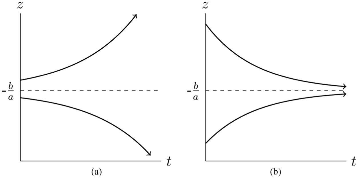
The behavior of solutions to differential equation 2.Note. (a) The unstable situation: a > 0. (b) The stable situation: a < 0.
Differential equation 2 describes a deterministic process; given an initial value
Let

where
Its initial value is zero:
Its sample paths have no “jumps” (or more formally,
It has independent increments
Here,
Combining the first and third property shows that
The Wiener process

where the second integral is an Itô stochastic integral (Øksendal 2000). An intuitive interpretation of equations 4 and 5 is that in a small time interval of length

Unlike

and variance

A derivation of equations 6 through 8 and further background on linear stochastic differential equations can be found in Mikosch (1998). In the case
Figure 2 explores stochastic differential equation 4 with
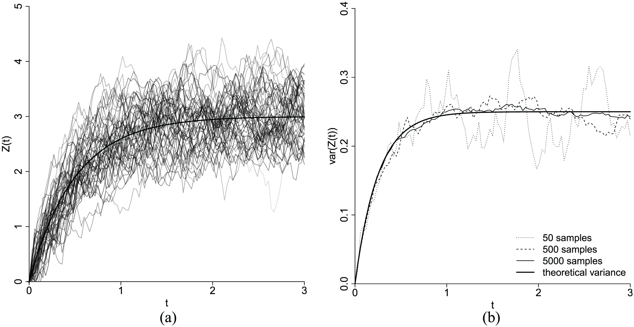
Exploring stochastic differential equation 4 with
3. Stochastic Actor-Oriented Model
The stochastic actor-oriented model represents network and attribute coevolution as an emergent group-level result of interdependent attribute changes and network changes (Snijders 2001; Snijders et al. 2007). One important characteristic of the model is its assumption that changes occur continuously in time. This means that in a real-valued time interval, changes can occur at any time point. The models discussed by Snijders (2001) and Snijders et al. (2007) are defined for discrete outcome spaces so that a change is always a discrete jump (one tie change or one category change in an attribute value) and on a finite interval only finitely many jumps will occur.
In the stochastic actor-oriented model, we assume that the observations of the network and actor attributes at discrete time points are the outcomes of an underlying continuous-time Markov process. In the current extension, we model the network evolution by a continous-time Markov chain (Norris 1997) and the evolution of a continuous actor attribute by a stochastic differential equation. These model components are discussed in Sections 3.2 and 3.3. Both processes satisfy the Markov property: Given their current state, the probability distribution of future states of the processes is independent of their past states. The Markov chain and the stochastic differential equation together constitute the network-attribute coevolution model (Section 3.4). In Section 3.1, we introduce the necessary notation.
3.1. Notation and Data Structure
The outcome variables for which the coevolution model is defined are the dynamic network and the dynamic actor attributes. The network is defined by its node set
The actor attributes are continuous variables, and they are measured on an interval scale. We will specify the stochastic actor-oriented model for a single coevolving continuous attribute, but extension to multivariate attributes is straightforward (Niezink and Snijders 2017). The vector
The data we consider are network-attribute panel data; the network and the attribute data are collected at two or more points
3.2. Network Evolution Model
We include here a short definition of the stochastic actor-oriented model. For a detailed discussion, see Snijders (2001, 2005, 2017b). A characteristic property of the model is its actor-oriented architecture. Changes in the network are modeled as choices made by actors about their outgoing ties. In other words, actors control the ties they send. We assume that at any given moment, all actors act conditionally independently of each other given the current state of the network and attributes of all actors. Moreover, actors are assumed to make only one tie change at a time. Similar to many other agent-based models, the model is based on local rules for actor behavior. It combines the strengths of agent-based simulation and statistical modeling (Snijders and Steglich 2015).
The stochastic actor-oriented model decomposes the network evolution process into two stochastic subprocesses. The first subprocess models the speed by which the network changes or, more precisely, the rate at which each actor in the network gets an opportunity to change one of their outgoing ties. The second subprocess models the mechanisms that determine which particular tie is changed when the opportunity arises. In the following, we specify both subprocesses.
For each actor
If actor
The choice of actor

also known as the multinomial logit model (McFadden 1974). This model can be obtained as the result of myopic stochastic optimization. The objective function is defined as a weighted sum of network effects

Parameter
The model for the dynamics of discrete actor behavior is defined analogously to the network evolution model (Snijders et al. 2007), with a behavior rate function and objective function. In the discrete behavior model, once actors get the opportunity to change their behavior, they can either increase or decrease their attribute value by 1 or keep the value constant. Choice probabilities are defined by a multinomial logit model, as in equation 9. Like the network, the actors’ attribute values are modeled as evolving in the smallest steps possible.
3.3. Continuous Attribute Evolution Model
Stochastic differential equation 4 describes the change in an attribute, but it does not include any information on what may have brought this change about. In our model, the dynamics of the attribute of an actor

If
The parameters in vector
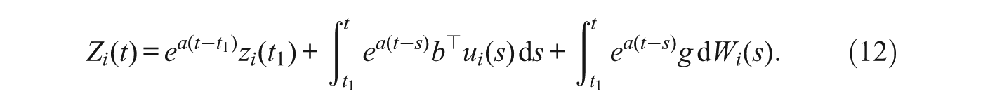
Equation 11 can be used to study the evolution of actor attributes between two measurements. However, when we are interested in modeling data from more than two measurement moments, we use the alternative specification,

where
3.3.1. Network Effects on Attribute Evolution
The effects discussed in the previous section are examples of exogenous effects. However, network-attribute coevolution studies usually focus on how the local network environments of actors and the characteristics of the actors to whom they are connected (i.e., their “alters”) affect their attribute dynamics. For example, the number of friends a student has or the self-esteem of his or her friends may affect that student’s self-esteem. We can model how actors are influenced by their alters in various ways, combining information on the current network state and the alters’ current attribute values.
Table 1 gives an overview of some network effects on attribute dynamics that have been implemented so far. For each of the effects, we give an example hypothesis in the context of the study discussed in Section 1. The actor’s network position itself may influence his or her behavior: For example, the indegree, outdegree, or reciprocated degree might lead to an increase or decrease in the value of the attribute. Degree-related effects can be considered in their raw form or in a transformation (e.g., Steglich et al. 2010). If the effect of an additional tie decreases with the number of ties an actor already has, this can be accounted for by a square root transformation. Especially for a right-skewed degree distribution, where some actors have a very high degree, such a transformation is natural.
Network-Dependent Effects Currently Implemented for Modeling Continuous Attribute Dynamics
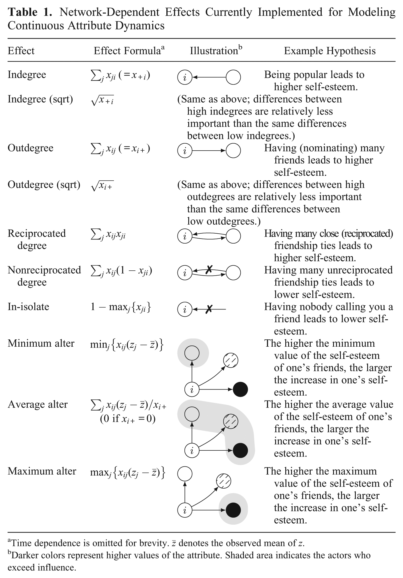
Time dependence is omitted for brevity.
Darker colors represent higher values of the attribute. Shaded area indicates the actors who exceed influence.
Actors may be affected by the attribute values of their alters. Three remarks about social influence may be noted here. First, we use the term social influence generally for all ways in which the network combined with the behavior of other actors in the network affects the behavior of actors. This is more general than the narrower meaning of social influence that refers only to ways in which the behavior of the influencing actor becomes more similar to the behavior of the actor being influenced, and it is illustrated in the following for some of the effects. Second, while some theories of social influence are formulated in terms of one actor who is being influenced by one other actor, neglecting third and additional actors, because of the empirical goals in coevolution studies, we must necessarily keep in mind that, in most cases, actors are surrounded by several other actors. The behavior of the focal actor is potentially influenced by all actors who are tied to the focal actor, and an aggregation step is necessary from the level of ties to the level of the personal network. Third, we interpret the tie from
The theoretical mechanisms behind social influence can vary by context. The choice to model influence by a particular effect is thus a theoretical one. Influence effects will have to reflect theories and potential mechanisms that could apply to the phenomenon being analyzed. Table 1 shows three examples of influence effects. As the corresponding hypotheses in the context of self-esteem could be artificial in some cases, we will discuss them instead for deviant behavior. The attribute-related influence effects in Table 1 are centered by the mean observed attribute value
Having at least one friend who is not involved in deviant behavior may keep a person on the straight and narrow. In this case, a person’s score on a deviance scale could increase when his or her least deviant friend becomes more deviant (minimum alter effect). If the least deviant friend of individual A is less deviant than the least deviant friend of individual B and this results in a higher increase in deviance of B than of A, we can consider this a form of social influence.
An alternative could be that having at least one deviant friend has a large impact on someone’s deviant behavior. In this case, a person’s deviance score could increase when his or her most deviant friend becomes more deviant (maximum alter effect). This may lead a person to deviate from the norm in his or her friendship group. Social influence thus does not necessarily imply that actors become more similar to their friends over time. Note that the person who is the least or most deviant friend may change over time.
A third possibility is that a person is affected by the average deviance level of his or her friends (average alter effect). In this case, the positive effect of the nondeviant individuals and the negative effect of the deviant individuals are assumed to even each other out. The average alter effect is a common operationalization of social influence in studies using the stochastic actor-oriented model. The idea of using a (weighted) average alter effect to model influence goes back to classical sociological models (e.g., Abelson 1964; French 1956); see Flache et al. (2017) for a recent overview of formal models of social influence.
This list can be extended with many other effects. A large variety of these have already been defined for discrete attribute variables in the stochastic actor-oriented modeling framework (Ripley et al. 2018), and many of these allow for a straightforward generalization to the case of continuous attributes. For example, in the discrete attribute evolution model, the total in-alter effect is defined by actor
Note that the effects in the discrete model are interpreted as effects of the type of a utility, or negative potential, whereas in our model, it is of the type of a derivative. This is why the effects in the discrete model have the additional factor
3.3.2. Discrete-Time Consequences
Stochastic differential equations describe how continuous variables may evolve over time. They express a rate of change. However, observations are usually made at discrete time points. The distribution of the continuous variables at a certain time point is fully determined by the stochastic differential equation and the initial conditions, yet for most models, it is impossible to derive an explicit expression for this distribution. Bergstrom (1984) addressed this problem for systems of linear stochastic differential equations that model the coevolution of multiple continuous variables. He showed that under certain conditions, discrete-time observations exactly satisfy a system of stochastic difference equations. His so-called exact discrete model links the discrete-time parameters with the continuous-time parameters.
Equation 11 is the one-dimensional case of the model addressed by Bergstrom (1984). For this model, the exact discrete model reduces to an expression very similar to what we have seen in Section 2 on stochastic differential equations (e.g., see Oud and Jansen 2000). Let

where

For equation 13, modeling attribute dynamics based on more than two measurement moments, these coefficients are given by

In the derivation of difference equation 14, it is assumed that the
3.4. Integration of Network and Attribute Model
The network-attribute coevolution model is specified by the rates
In the coevolution model, the network evolves in “jumps” of one tie change, while the actor attributes evolve gradually. The Markov chain for the network evolution is fully specified by its infinitesimal generator matrix or intensity matrix

The diagonal entries of
Note that the off-diagonal entries that are nonzero correspond to network changes that involve only a single tie change. The waiting time until a transition out of state

This transition probability decomposes into the probability
1. Initialize: set
2. Sample
While
3. Update
4. Select actor
5. Select alter
6. Update: set
7. Sample a new
In the simulation scheme, there is a waiting time until a new network change is drawn (Steps 2 and 7), the actor attributes are updated (Step 3), the actor who will make a change is determined (Step 4), and the tie change is determined (Step 5). To reach
For simulation purposes, we assume that
If the
For very small networks with little change between observations, deviations in simulated attribute values will be larger. Splitting up the time interval
4. Effect Sizes
An important difficulty in working with stochastic actor-oriented models is the interpretation of parameters in a nonstandardized fashion. The parameters in the standard stochastic actor-oriented model for discrete behavior variables are nonstandardized coefficients in the multinomial logit model for the discrete changes in network and behavior. Multinomial logit model parameters are difficult to interpret, and their arrangement in this complex network model adds to the difficulties in interpretation. The relation of the stochastic differential equation model to linear regression can be used to have a better understanding of the parameters, with analogues of the proportion of explained variance and effect sizes.
4.1. Parameter Interpretation
Estimated parameters in attribute dynamics models (equations 11 and 13) represent the strength of effects on change in attribute values. Using the exact discrete model (see again Section 3.3.2), we can assess the implication of this model for expected change trajectories. Considering these change trajectories helps in interpreting parameter sizes.
Assume, by way of example, that in a simple coevolution model, the stochastic differential equation for evolution of a mean-centered attribute variable was given by

where

The parameters in equation 13, for more than two measurement moments, can be interpreted along the same lines as discussed in the following.
To simplify parameter interpretation, we approximate the indegree
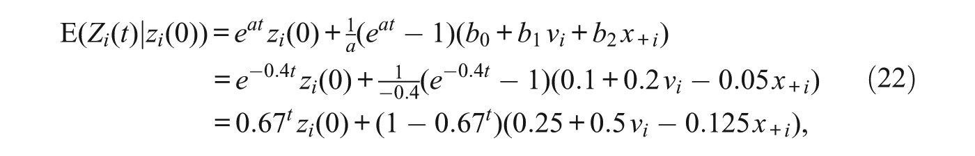
where
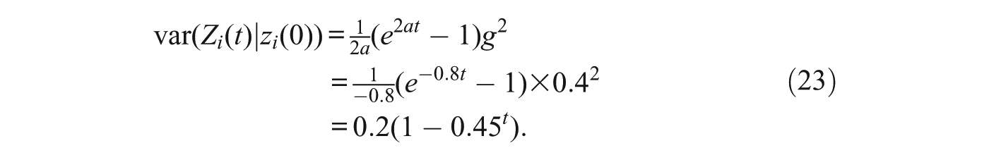
Figure 3 visualizes the attribute dynamics given in equation 21. Figure 3a shows the extent of the variation in 50 sample trajectories for one actor. Note that we assume the variation to be the same for all actors, much like the homoscedasticity assumption in a regression analysis. Figure 3b shows the effect of an actor’s indegree on his or her attribute value. The differences between the trajectories for actors with different indegrees are small, especially considering the amount of random variation in Figure 3a.
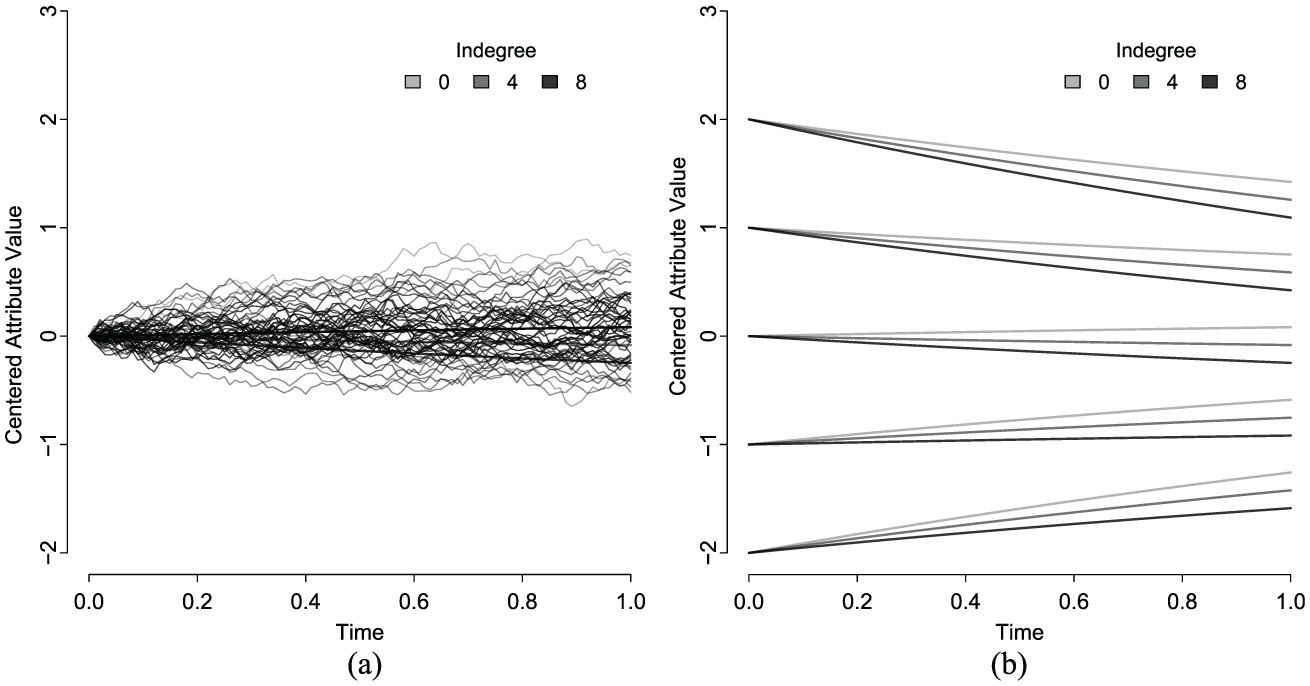
Visualization of the attribute dynamics given in equation 21.Note. (a) The mean trajectory and 50 sample paths for an actor with an average initial attribute value, vi = 0 and indegree 0. (b) The mean trajectories for actors with vi = 0 for various initial attribute and indegree values.
As shown by the previous exposition, the continuous-time parameters are best interpreted in terms of their discrete-time consequences. Interpreting the value of 0.2 for the covariate parameter
Nevertheless, the processes we study are often far from being in equilibrium, and focusing on the equilibrium coefficients may not be all-revealing. Therefore, we also evaluate the discrete-time consequence of the continuous-time model after one observation period. Since in the model the time between consecutive measurements is set to 1, the exact discrete model yields

where the indegree is again taken to be constant. Moreover,
Filling out observation interval length
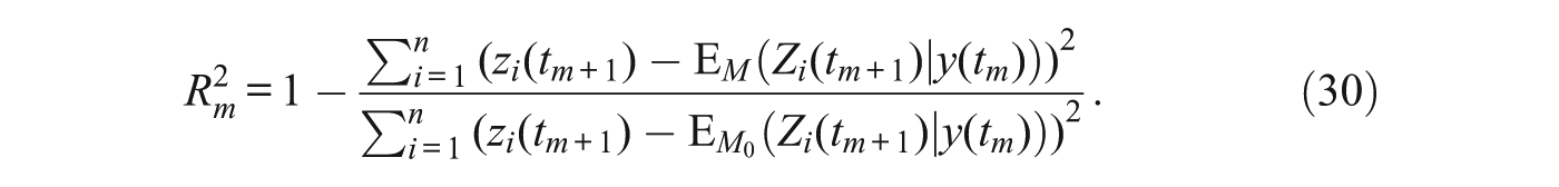
4.2. Explained Variance
For stochastic actor-oriented models for network evolution, Snijders (2004) proposed a measure of explained variation using information theory. The measure is based on the entropy (Shannon 1984) in the probabilities involved in actors’ network change decisions, where a low entropy indicates a high degree of certainty in the outcomes of network changes and thus high explained variation. Unfortunately, the measure is not easily interpretable and is therefore hardly applied.
In linear regression, the proportion of explained variance, usually denoted by

where
For a linear regression model

We can consider
The same ideas can be applied to define a proportion of explained variance in the context of the continuous attribute model presented here. For the stochastic differential equation, the null model

for model equation 11 and

for model equation 13. This quantity can be computed using estimates of

can be estimated based on simulations of the coevolution model under study. In line with equation 26, the proportional reduction in unexplained variance, or the proportional reduction in prediction error for period
Note that if the attribute dynamics do not depend on network characteristics, we can estimate the attribute model straightforwardly using the exact discrete model and likelihood maximization and determine the explained variance as in a standard regression model. This is also possible if the network is constant and the model contains only purely structural and covariate effects. Note also that while
5. The Coevolution of Friendship, Alcohol Use, and Self-Esteem
This section investigates the interplay of friendship dynamics and the dynamics of alcohol use and self-esteem among adolescents. We use a stochastic actor-oriented model to study the coevolution of a network (friendship), a discrete actor variable (alcohol use), and a continuous actor variable (self-esteem). Steglich et al. (2010) advocated the use of the stochastic actor-oriented model to distinguish peer selection from social influence, two social mechanisms leading to network autocorrelation. Since then, many researchers have followed in disentangling selection and influence in various contexts. Nevertheless, few studies have considered the conditions under which selection and influence occur. Some actors may be more susceptible to these processes than others. Schaefer (2016) studied whether adolescents with particular risk factors, such as having low self-control or weak attachments to protective institutions (e.g., family or school), have a greater risk of befriending substance-using peers, who could later become a source of negative influence. However, not all adolescents may be equally suspectible to influence. Discovering the characteristics of the adolescents who are most susceptible to influence of their peers is important. Compared with trying to change a person’s friendship ties, interventions aimed at individidual characteristics are easier to implement (e.g., in a personal skills training context) and often more ethical.
In this study, we consider self-esteem as a potential buffer for the effect of peers on the behavior of adolescents. Adolescents with high self-esteem may be less susceptible to influence than their low self-esteem peers. We reanalyze the data studied by Steglich et al. (2010), considering the role of self-esteem in friendship and alcohol use dynamics. Furthermore, we assess the effects of popularity and alcohol use on self-esteem.
5.1. Data
The data are part of the Teenage Friends and Lifestyle Study (Pearson and Mitchell 2000; Pearson and West 2003), which aimed to identify the mechanisms by which attitudes toward smoking and smoking behavior itself change during early to midadolescence. Students in a cohort at a secondary school in Glasgow were followed over a two-year period (February 1995–January 1997). Of the 160 students in the cohort, aged 12 to 13 at the beginning of the study, 150, 146, and 137 participated at the first, second, and third measurement, respectively. We include all 160 students in the analysis, taking into account the changes in composition. The students were asked to nominate up to six friends from their cohort and answer questions about various behaviors and attitudes, including social relations and risk behavior. Previous studies of these data have addressed the coevolution of friendship and taste in music (Steglich, Snijders, and West 2006) and that of friendship and cannabis use (Pearson, Steglich, and Snijders 2006).
Alcohol consumption frequency was measured on a scale ranging from 1 (not at all) to 5 (more than once a week). Self-esteem was measured by a 10-item scale, based on Rosenberg (1941), with items such as “I am easy to like” and “I often wish I was someone else.” The items were measured on a scale ranging from 0 (strongly agree) to 3 (strongly disagree). The self-esteem score was calculated as the average over all items after reverse coding the negatively formulated items so that a high score corresponds to high self-esteem. Students also reported their sex (0 = male, 1 = female).
For descriptive statistics of the friendship network and alcohol use data, we refer to Steglich et al. (2010). The distribution of the self-esteem data at the three measurements is shown in Figure 4, where a slight increase of self-esteem can be seen over time. The average self-esteem score increases from 1.63 at the first measurement to 1.68 at the second and 1.79 at the third. For the analysis, self-esteem is centered by subtracting the overall mean of 1.70.
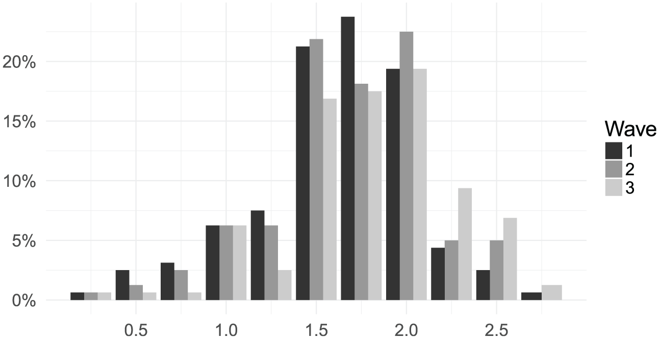
Observed distribution of self-esteem at the three measurements.
5.2. Model
In order to study the effect of self-esteem on students’ susceptibility to peer influence on drinking behavior, we need to model self-esteem as a coevolving dependent variable. We thus study the coevolution of friendship, alcohol use, and self-esteem, modeling the evolution of a network, a discrete actor variable, and a continuous actor variable simultaneously. Two models are estimated. In the first model, the “evolution model,” we study the dynamics of friendship, alcohol use, and self-esteem separately. Formally, this can be done in one joint model, where the three dependent variables are specified as being mutually independent. The interplay among the three dependent variables is studied in the second model, the “coevolution model.” In this model, we assess through an interaction term whether students’ susceptibility to peer influence on alcohol use depends on their level of self-esteem. We estimate parameters by the methods of moments. See Appendix A and Appendix B for a discussion of parameter estimation and standard error estimation. Missing data are imputed for simulation purposes but disregarded in the computation of the statistics of the moment equations (Huisman and Steglich 2008; Ripley et al. 2018).
5.2.1. Friendship Dynamics
In the friendship dynamics part of the model, we first include structural effects in the objective function. The outdegree effect represents the balance between creating and dropping ties, and it is like an intercept. We also model the tendency to reciprocate friendship nominations (reciprocity) and the tendency for actors to befriend the friends of their friends (transitivity) and the interaction of these two effects. Reciprocity and transitivity usually play an important role in friendship dynamics, but their effect is mostly not additive, resulting in a negative interaction effect. As explained by Block (2015), the tendency toward reciprocation of friendships within transitive groups is usually lower than it is outside of transitive groups.
Apart from the basic outdegree effect, we include three other degree-related effects: the effect of current popularity (number of incoming ties, indegree) on receiving friendship nominations (indegree popularity) and sending friendship nominations (indegree activity) and the effect of current network activity (number of outgoing ties, outdegree) on nominating friends (outdegree activity).
We also assess the effects of alcohol use and self-esteem on friendship dynamics by including their ego effects and alter effect in the network objective function. These effects measure the differential tendency of students with higher values to nominate friends and receive friendship nominations, respectively. We model the differential attractiveness of students with high self-esteem to other students with high self-esteem by an interaction effect of ego’s and alter’s self-esteem scores. We also include the interaction of ego’s and alter’s alcohol use. Finally, we account for effects of gender (ego, alter, same) on the dynamics of the friendship network.
5.2.2. Self-esteem Dynamics
In the coevolution model, we also include, apart from the feedback, intercept and scale parameters, the effect of alcohol use on change in self-esteem and that of popularity, as measured by a student’s indegree in the friendship network. The stochastic differential equation for the self-esteem dynamics in period

where
Since we analyze the centered esteem scores instead of the original ones, we can meaningfully interpret the intercept parameter
5.2.3. Alcohol Use Dynamics
The alcohol use dynamics, like the friendship dynamics, are modeled in the discrete Markov chain framework. The base components of the alcohol use objective function are the linear and quadratic shape effects, which capture the basic shape of the alcohol use distribution. The model contains one main friendship-related peer influence component: the effect of the average alcohol use among friends on adolescent alcohol use (average alter effect). As we are interested in whether self-esteem moderates the strength of peer influence on alcohol use, we include the interaction effect of ego’s self-esteem and the average alter effect on alcohol use. We also take into account the potential direct effect of self-esteem on alcohol use.
5.3. Results
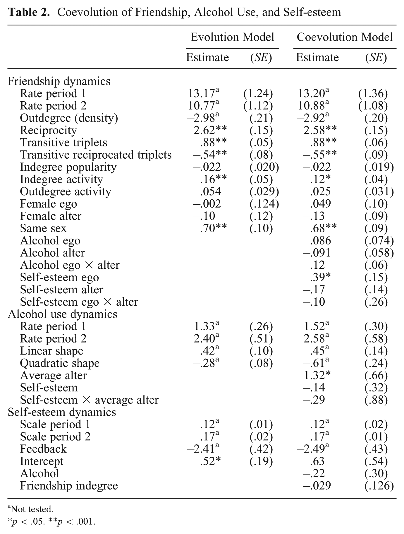
The results for the evolution model and the coevolution model are shown in Table 2. Based on 1,000 simulations of the coevolution model and using the procedure developed by Lospinoso (2012) implemented in the RSiena package (Ripley et al. 2018), we can conclude that the model fits the network data well in terms of its outdegree distribution (p = .10), indegree distribution (p = .60), and triad census (p = .09). The alcohol and self-esteem data also fit fairly well, as shown in Figure 5. In the following discussion, we first explain the friendship network dynamics results and then the results for the alcohol use and self-esteem dynamics.
Coevolution of Friendship, Alcohol Use, and Self-esteem
Not tested.
p < .05. **p < .001.
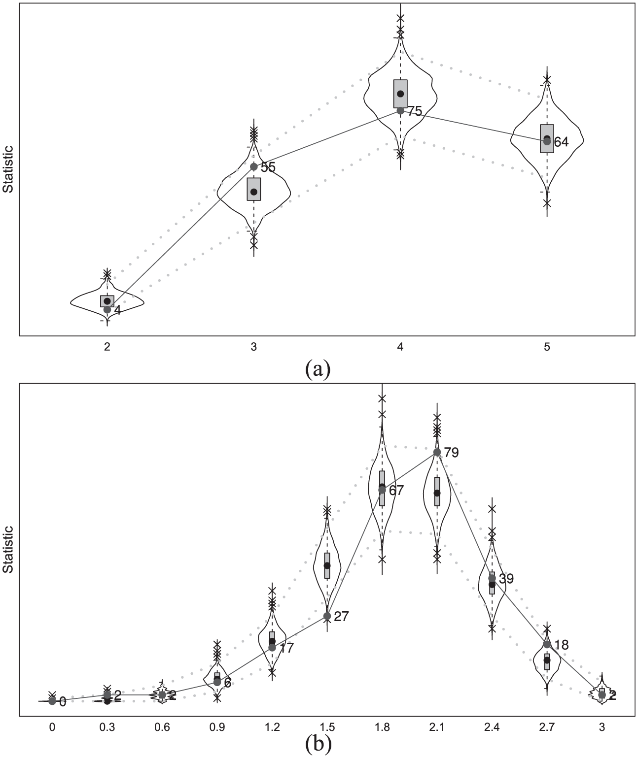
Goodness-of-fit plots for alcohol use and self-esteem distribution based on 1,000 data sets simulated with the coevolution model parameters (see Table 2).Note. (a) Alcohol use distribution, p = .47. (b) Self-esteem distribution, p = .07. The numbers and solid lines represent the values observed at the end of periods 1 and 2.
We find that students with higher self-esteem tend to send more friendship nominations (self-esteem ego). Apart from this, students’ self-esteem seems to have little effect on the evolution of friendship ties, and the same holds for their alcohol use.
The estimates of the purely structural effects do not change much when the alcohol and self-esteem effects are included in the model. Students have a tendency to reciprocate friendship ties and prefer relationships with their friends’ friends (positive transitive triplets), but these effects are not additive (negative transitive reciprocated triplets). Moreover, students who are mentioned by many others as a friend have a lower tendency to nominate others as friends (negative indegree activity). Finally, we find strong evidence of homophily based on sex (positive same gender).
Peer influence is the social mechanism of key interest in our model of how students’ alcohol use changes over time. Table 2 shows that friends indeed have an effect on students’ alcohol intake (positive average alter). However, we find no evidence that susceptibility to peer influence differs by students’ self-esteem level (self-esteem × average alter). Students’ self-esteem does not appear to directly affect their alcohol use either. The results for the full model without the self-esteem and average similarity interaction effect—not presented here—are comparable to those for the coevolution model. In this model, the average alter effect is 1.34 (SE = 0.60), and the effect of self-esteem on alcohol use is –0.13 (SE = 0.33).
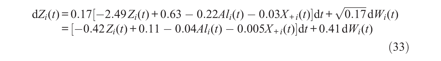
Considering the self-esteem dynamics model results for the evolution model, we find that self-esteem significantly increases over the course of the study period (positive intercept). This corresponds to the distributions shown in Figure 4. The sizes of the intercept and feedback parameter and the scale parameter for period 2 can be interpreted by considering again Figure 3a. The parameters in the estimated differential equation

are very similar to those used for simulating the trajectories in Figure 3a. The figure depicts the expected trajectory and gives an idea about the amount of uncertainty on the trajectory for a student with a self-esteem score of 1.70 (the overall observed average) at the beginning of period 2. The size of the random fluctuations is similar in the coevolution model and quite large compared with the effects of alcohol use or popularity on self-esteem. To see this, compare the parameter sizes of alcohol use and self-esteem in the estimated coevolution model
for period 2 with the size of the popularity effect (
Table 2 also shows that there is no significant effect of popularity or alcohol use on self-esteem in the coevolution model. Moreover, popularity and alcohol use do not improve the model in terms of explained variance for self-esteem. Based on 1,000 Monte Carlo simulations of the coevolution process, we find that for periods 1 and 2 the explained variance estimates are
6. Discussion
This article presented a model for studying the coevolution of social networks and continuous attributes of network actors. The model extends the stochastic actor-oriented model for network evolution (Snijders 2001). The model discussed by Snijders et al. (2007) and Steglich et al. (2010) requires continuous attributes to be discretized, but in the model presented here, this is no longer necessary. Continuous attributes arise as representations not only for variables that are “really” continuous, such as income or length or weight dimensions, but also as results of multi-item scales such as psychological constructs, approximations to counts that have a wide range, and measured variables that are aggregations of many decisions and circumstances such as performance of individuals or companies.
We illustrated the proposed method with a study of the dynamics of friendship, alcohol use, and self-esteem among adolescents. This study advocates the elaboration of the “selection versus influence” narrative by considering under which circumstances peer selection based on shared characteristics and social influence occur. In the study, we consider whether the susceptibility of students to peer influence on alcohol use differs according to their self-esteem, but we do not find evidence for such differential susceptibility. This example was presented not so much because of its substantive results—the sample size is on the low side for such a question—but as an illustration of the type of research question for which this method could be used.
The continuous attribute dynamics are modeled by a linear stochastic differential equation. We showed how given estimated parameters, formulas and figures can be of help in understanding continuous actor attribute dynamics and in the communication of results. Moreover, stochastic differential equations give us access not only to average trajectories but also to information about the variability in these trajectories. Comparable information for discrete dynamic actor attributes in the stochastic actor-oriented model is not obtained in as straightforward an approach.
The linear stochastic differential equation model closely resembles (and in some cases is equivalent to) an ordinary linear regression model. Many generalizations of the ordinary regression model can be implemented for the stochastic differential equation as well. Examples include random effect and latent variable models. In this article, we assumed that the network represents one group. A study of coevolution processes in a sample of networks (e.g., Knecht et al. 2011) would require a multilevel extension of the method proposed here.
The resemblance of the attribute evolution model with the ordinary linear regression model at the same time instills awareness of potential modeling challenges. Questions about the validity of the linearity and homoscedasticity assumption follow naturally. Moreover, although discretization of continuous variables is no longer necessary due to the model extension, transformation might be. This transformation could be aimed at improving the validity of the distributional assumptions of the model, but it could also have a substantive objective. For example, the perception of the importance of a one-point change in an attribute value may differ in different ranges of the attribute spectrum. We can study transformations of continuous actor attributes to ensure that the assumption of an interval scale is reasonable.
While the network and discrete behavior coevolution model (Snijders et al. 2007) assumed that the behavior variable has a lower and upper bound, no such assumption was made for the continuous behavior model presented in this article. If a continuous variable is studied that takes values only in a certain range, simulated behavior trajectories will mostly lie in this range but also partly outside it. A stochastic differential equation model with reflecting boundary conditions could be developed to counter this.
The choice between a coevolution model with a continuous versus a discrete attribute is not merely a methodological issue or a matter of data, but it depends on the research question under study. For example, even in the case when the exact amount of alcohol consumed by students in a high school is known, drinking behavior is best modeled on a binary scale when the research is about peer influence on the onset of drinking. An onset model (Greenan 2015) in the stochastic actor-oriented modeling framework would in this case match the research question better than a model with an ordinal or continuous drinking variable. The differences in results and model properties between the models for continuous attributes and discretized continuous attributes require further exploration.
Footnotes
Appendix A
Appendix B
Acknowledgements
We gratefully acknowledge the editor and the anonymous reviewers as well as Christian Steglich for helpful comments and suggestions.
Funding
The first author was funded by the Netherlands Organization for Scientific Research (NWO) under grant 406-12-165.