Challenges in Multilevel Modelling: Cross-Group Measurement Noninvariance and Measurement Errors. A Monte Carlo Simulation Study

Abstract

Multilevel modelling (MM) is widely utilized in the social sciences, with over 20% of articles in leading sociological journals employing this technique. Despite its prevalence, few studies address whether the variables used in MM are invariant across groups or allow to construct reliable indicators. This study investigates the effects of both measurement noninvariance and random measurement error on MM using Monte Carlo simulations. Our findings reveal significant biases in MM results when random measurement errors are overlooked. Attaining high reliability in the indicators – above 0.94 – can mitigate these biases. While measurement noninvariance introduces bias in MM, its impact is smaller compared to that of the bias caused by unaddressed measurement error. Multilevel structural equation modelling (SEM), which controls for random measurement errors, performs effectively in complete measurement invariance (MI) scenarios. However, the absence of MI can create significant challenges. While multilevel SEM is a powerful analytical tool, it is not immune to the effects of MI assumption violations.

The relationship between individuals and society has been a central focus of sociological research since the discipline's inception. Multilevel modelling (MM; Hox, Moerbeek, and van der Schoot 2018; Snijders and Bosker 2012) has emerged as a key tool for studying the interplay between contextual (macro) phenomena and individual (micro) processes. A part of the popularity of MM is entrenched in the growing availability of large-scale cross-country surveys that provide researchers with the possibility to analyze rich and easily available data, such as the European Social Survey (ESS), the International Social Survey Programme (ISSP), the World Values Study (WVS), or the Programme for International Student Assessment (PISA), just to name a few. Indeed, Heisig, Schaeffer, and Giesecke (2017) demonstrated that more than 20% of the articles published between 2011 and 2014 in three leading sociological journals – American Journal of Sociology, American Sociological Review, and European Sociological Review – utilized MM as a tool to test their hypotheses.

However, virtually none of these articles addressed a potentially crucial assumption when performing MM: The cross-country (or cross-group) comparability of the variables used in the analysis, commonly referred to as the measurement invariance (MI) or equivalence assumption. Furthermore, most studies employing MM overlooked another crucial and related issue – that of random measurement errors. Building on the analysis by Heisig, Schaeffer, and Giesecke (2017), we examined the prevalence of testing for MI and accounting for measurement errors in published articles using MM. To do so, we screened three leading international journals with solid impact factors (IFs): American Sociological Review (IF 2020: 6.372), American Journal of Sociology (IF 2020: 4.688), and the European Sociological Review (IF 2020: 2.960). Table 1 reports the actual percentages of papers published in these three journals (N = 125) between 2015 and 2020 that reported the use of MM. Of the 49 articles (39.2%) that employed only observed variables or composite scores in MM, none tested whether MI was given. In addition, each of these articles implicitly assumed that the reliability of the scales was sufficiently high to avoid negatively impacting the estimation results (see Appendix 1 in the online Supplemental Material for the complete list of articles). Finally, only four (3.2%) of the 76 articles (60.8%) that used latent variables actually tested for MI.

Table 1.

Number (Percentage) of Papers Published in Three Leading Sociological Journals Using MM and Examining MI.

		With measurement invariance testing	Without measurement invariance testing	Overall
Only observed variables	With cross-level interactions	0 (0%)	24 (19.2%)	24 (19.2%)
	Without cross-level interactions	0 (0%)	25 (20%)	25 (20%)
With latent variables	With cross-level interactions	2 (1.6%)	54 (43.2%)	56 (44.8%)
	Without cross-level interactions	2 (1.6%)	18 (14.4%)	20 (16%)
	Overall	4 (3.2%)	121 (96.8%)	125 (100%)

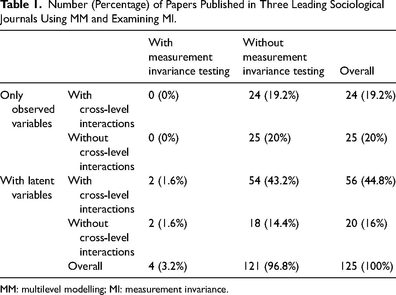
MM: multilevel modelling; MI: measurement invariance.

This neglect is unfortunate, as both measurement errors (Wooldridge 2010) and measurement noninvariance across groups (Leitgöb et al. 2023; Pokropek, Davidov, and Schmidt 2019) can severely bias estimates of statistical models (e.g., Pokropek 2015; Woodhouse, Goldstein, and Rasbash 1996). Previous research has shown that MI is essential for meaningful comparative sociological research, yet it is frequently violated in international survey data (Davidov et al. 2014). Lack of MI is likely to lead to incorrect conclusions when comparing specific parameters of interest – means or association measures such as regression coefficients or covariances – across countries or cultures (Van de Vijver 2011). However, is MI equally important for performing meaningful MM analysis, where the cross-group comparability of indicators is implicitly assumed?

Across a wide array of conditions, our Monte-Carlo experiments converge on a single, robust pattern: unmodelled random measurement error is the primary driver of distortion in multilevel estimates, dwarfing the impact of moderate violations of MI. Once reliability slips below a very demanding threshold (≈ 0.94), bias propagates through both fixed and random effects, undermining coefficient accuracy and inflating Type I error rates. Conversely, when reliability is exceptionally high, multilevel models prove surprisingly resilient to partial or moderate MI breaches – especially if those breaches are confined to a minority of groups or items. Yet even under optimal reliability, extensive scalar non-invariance (i.e., many intercepts differing across groups) reintroduces appreciable bias and erodes interval coverage. Latent-variable specifications (multilevel SEM) substantially curb measurement-error bias, but they, too, become vulnerable when large swaths of the measurement model violate invariance. Hence, neither high reliability alone nor latent modelling alone fully inoculates multilevel analysis against inferential error.

The Structure and Aims of the Study

We begin by summarizing the concept of measurement error and its significance in MM. Next, we discuss MI, highlighting its relevance for MM. Subsequently, we introduce our simulation method, detail its application, and present the results. The simulation study examines three specific and realistic scenarios. The first involves estimating MM regression using observed indicators (factor scores) under conditions where MI is given and measurement error is ignored. This scenario explores the impact of measurement error on MM estimates. In the second scenario, we assess how measurement noninvariance affects the results in MM regression. Finally, the third scenario examines the implications of measurement noninvariance in MM structural equation modelling (SEM; Heck and Thomas 2015; Hox, Moerbeek, and van der Schoot 2018; Meuleman 2019; Muthén 1994; Rabe-Hesketh, Skrondal, and Pickles 2004), of which MM regression is a special case.

We present the results of the Monte Carlo simulations for several key parameters of interest in MM: (1) individual-level effects (level 1), (2) higher-level effects (level 2), and (3) cross-level interaction effects. This analysis reveals whether, and under which conditions, conclusions in MM remain valid, even when MI is not supported by the data and the reliability of indicators is not perfect. To the best of our knowledge, this study is the first to examine the significance of MI for MM and the combined relevance of MI and measurement error. We conclude with a summary of the main findings.

There is no Measurement Without Error

In scientific research, it is a fundamental truth that virtually no measurement is entirely free from error. This principle extends beyond the social sciences, permeating all disciplines that rely on empirical data. The inherent uncertainty in measurements underscores the need for rigorous consideration and analysis in all scientific endeavours. To address this issue, researchers have advocated for the use of composite indicators, particularly in questionnaires, as these allow for multiple measures of the same construct, thereby increasing reliability.

These composite scores are typically constructed using multiple indicators that reflect an individual's beliefs or attitudes. Reliability of these indicators is often assessed using measures like Cronbach's alpha (Cronbach 1951) or McDonald's omega (Raykov 2011). When these indicators demonstrate high reliability, they are frequently used as variables in MM and other types of analyses. However, accounting for random measurement error in sociological studies in general, and particularly in MM, has been more the exception than the rule (Saris and Gallhofer 2014). This is unfortunate because low reliability due to random measurement errors can lead to severely biased research findings.

A common bias introduced by measurement error is attenuation bias (Pokropek 2015), where low reliability leads to an underestimation of correlations and regression coefficients. Specifically, the parameters of regression models (including MM parameters) will be downwardly biased, inversely proportional to the reliability of the independent variables. To address known reliability issues, some researchers have proposed adjusting coefficients by dividing them by the reliability factor (see Woodhouse, Goldstein, and Rasbash 1996). However, in more complex modelling scenarios, addressing measurement error and bias becomes increasingly challenging, as both the direction of bias and suitable analytical corrections are often unknown (Bollen 1989). For instance, Pokropek (2015) demonstrated that ignoring measurement error in MM typically leads to significant upward biases, creating ‘phantom effects’ indicating positive significant effects even when – in reality – they do not exist.

To effectively account for measurement errors in complex modelling, SEM and its extension, MM SEM, have been developed. These methodologies enable researchers to incorporate and adjust measurement errors within MM models, resulting in more accurate and reliable conclusions (Muthén 1994). However, despite the availability of these advanced tools, they are rarely applied in the social sciences. Dedrick et al. (2009) analyzed 99 articles on MM from 13 peer-reviewed journals in education and the social sciences. Their findings showed that only 18 articles accounted for measurement errors in their models. Most studies relied on observed composite scores without adequately considering the potential impact of measurement error on the results of their MM analysis. This oversight could lead to significant misinterpretations and flawed conclusions.

What is MI and why Does it Matter?

When a study involves comparisons, a lack of comparability – known as measurement noninvariance – becomes a potential source of bias. Horn and McArdle (1992) define MI as a situation where ‘under different conditions of observing and studying phenomena, measurement operations yield measures of the same attribute’ (117). Research has shown that measurements are only comparable across groups if the response mechanisms are the same across those groups (e.g., Davidov et al. 2014; Meredith 1993; Steenkamp and Baumgartner 1998; Vandenberg and Lance 2000). In other words, MI implies that two respondents with the same level of a particular trait score similarly on the indicators measuring that trait, regardless of other characteristics (such as nationality or cultural background). When MI is absent, measurement instruments may assess the construct differently across groups, resulting in inequivalent measurements. Meredith (1993) demonstrated that this results in biased comparisons, because observed differences in measurement reflect not only variations in the true score of the trait but also disparities in response behaviours across groups. Consequently, cross-group differences may be methodological artefacts rather than a reflection of true differences. Similarly, the lack of observed differences in measurement can obscure true differences in the trait of interest.

Mellenbergh (1989) proposed formalizing the assumption of MI in terms of conditional independence:

$$f(U|\theta ,G=g)=f(U|\theta )$$

(1)

MI holds when the distribution of the response variable U, given the latent trait $\theta$ is conditionally independent of group membership G for a given group g. Only if this condition is fulfilled can the inferred differences between groups be attributed to real differences of the trait in the population rather than to group-specific differences in response behaviour (Byrne and van De Vijver 2010; Davidov et al. 2014).

This condition corresponds specifically to scalar MI in SEM. Scalar invariance requires that both the factor loadings λ and the intercepts ν are equal across groups: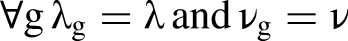

$$\mathrm{\forall }\mathrm{g}{\lambda }_{\mathrm{g}}=\lambda \mathrm{and}{\nu }_{\mathrm{g}}=\nu$$

Under scalar invariance, the measurement model for the observed variable U is expressed as:

$$U=\nu +\lambda \theta +\epsilon$$

(2)

Since both λ and ν are invariant across groups, the probability distribution f(U∣θ) is the same for all groups, satisfying Mellenbergh's conditional independence. In contrast, configural invariance allows both factor loadings and intercepts to vary across groups, while metric invariance requires equal factor loadings across groups but allows intercepts to differ. Only under scalar invariance does Mellenbergh's assumption hold, ensuring that observed group differences are attributable solely to differences in the latent trait θ, rather than to measurement differences across groups. If metric invariance is supported by the data, cross-group comparisons of unstandardized associations (unstandardized regression coefficients, covariances) between constructs of interest becomes meaningful (Steenkamp and Baumgartner 1998; Vandenberg and Lance 2000). However, comparing means across groups requires scalar invariance (Vandenberg and Lance 2000). Meuleman et al. (2022) and Leitgöb et al. (2023) emphasize the conceptual and theoretical importance of testing for MI to ensure valid measures, and they provide guidance on how to effectively examine MI.

In recent decades, both the methodological literature and applied social science research have witnessed a significant increase in studies examining the measurement properties and the cross-cultural equivalence of commonly used instruments. These instruments assess constructs such as basic human values, attitudes toward immigration, support of democracy, discrimination against minority groups, and national identification, among others (for a review, see, e.g., Davidov et al. 2014; Davidov, Muthén, and Schmidt 2018). Research has consistently shown that while lower levels of MI are often established, scalar invariance is rarely attained in practice. To address this issue, various solutions have been proposed, such as relying on partial invariance rather than full invariance (e.g., Pokropek, Davidov, and Schmidt 2019; Steenkamp and Baumgartner 1998), approximate invariance rather than full invariance (Muthén and Asparouhov 2013; Van De Schoot et al. 2013), or on an alignment optimization, which identifies the most reliable group means even in the absence of MI (Asparouhov and Muthén 2014; Pokropek, Lüdtke, and Robitzsch 2020a). Simulations conducted by Pokropek, Davidov, and Schmidt (2019) and Pokropek, Schmidt, and Davidov (2020b) demonstrate that, under certain conditions, these methods provide sufficient accuracy for drawing meaningful conclusions.

MM relies on estimating the heterogeneity in means (random intercepts) and regression coefficients (random slopes) across the groups involved in the analysis. The comparability of these groups across the macro units of analysis, in turn, depends on the presence of MI. Despite the availability of numerous methods, it is still the exception rather than the rule for studies employing MM analysis to examine their scales’ measurements in general, and their MI properties in particular. In the next section, we conduct Monte Carlo simulations to examine whether ignoring measurement errors and measurement noninvariance leads to bias in MM results.

Setup of the Simulation Study

This simulation study aims to evaluate the extent to which measurement errors – and, more specifically, measurement noninvariance – affect the effectiveness of MM in retrieving population parameters of interest. Using a Monte Carlo simulation approach, we defined population models with a multilevel data structure, including scenarios where measurement errors were given and MI assumptions were violated to varying degrees. Aims to evaluate (Bandalos and Gagne 2012). By comparing the retrieved parameters to the known population parameters, we evaluated the consequences of measurement errors and measurement noninvariance. This approach is well-established and widely used, with numerous practical examples examining MI (Kim et al. 2017; Meade and Lautenschlager 2004; Pokropek, Davidov, and Schmidt 2019, 2020b; Pokropek, Lüdtke, and Robitzsch 2020a; Yoon and Millsap 2007) as well as MM (Ferron, Farmer, and Owens 2010; Meuleman and Billiet 2009; Stegmueller 2013; Pokropek 2015).

The Monte-Carlo design utilized in this study comprises two analytically linked series. The first series applies conventional multilevel regression to factor scores, varying reliability (3, 5, 10, 15, 20 indicators) and degrees of MI. The second series re-estimates the same structural relations using full multilevel SEM; here, every construct is intentionally limited to three indicators for computational tractability. Consequently, design factors expressed as proportions of items (e.g., ‘1⁄3’ or ‘2⁄3’ non-invariant indicators) map onto one vs two items in the first series and, for comparability, onto proportional subsets in the second series (e.g., 5 vs 10 of 15 items).

The Population Model

Data for all simulations were generated using a relatively simple yet comprehensive model that contains parameters typically investigated in MM analyses in social science research (see Appendix 1 in the online Supplemental Material for a review). Our model specification is given below:

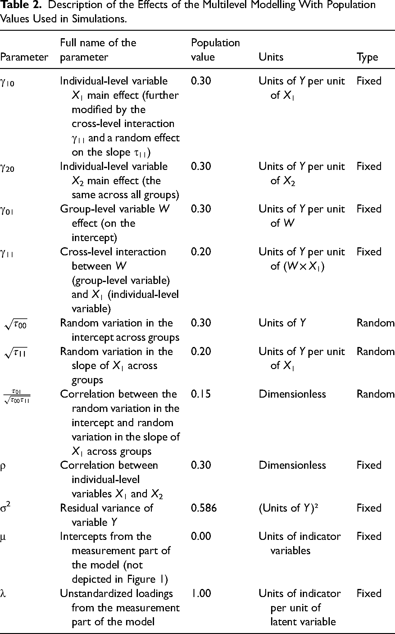
Hierarchical Form:

Level 1 (respondents):

$$Y_{ij}={\beta }_{0j}+{\beta }_{1j}{X}_{1ij}+{\beta }_{2j}{X}_{2ij}+r_{ij}$$

(3)

Level 2 (e.g., countries):

$${\beta }_{0j}={\gamma }_{00}+{\gamma }_{01}{W}_j+u_{0j}$$

(4)

$${\beta }_{1j}={\gamma }_{10}+{\gamma }_{11}{W}_j+u_{1j}$$

(5)

$${\beta }_{2j}={\gamma }_{20}$$

(6)

Combined Form:

$$Y_{ij}={\gamma }_{00}+{\gamma }_{01}{W}_j+{\gamma }_{10}{X}_{1ij}+{\gamma }_{11}{W}_j{X}_{1ij}+{\gamma }_{20}{X}_{2ij}+{\mu }_{0j}+{\mu }_{1j}{X}_{1ij}+r_{ij}$$

(7)

and

$$var(r_{ij})={\sigma }^2;var({\mu }_{0j})={\tau }_{00};var({\mu }_{1j})={\tau }_{11};cov({\mu }_{0j};{\mu }_{1j})={\tau }_{01}$$

(8\ndash10 )

$$cov(u_{0j},r_{ij})=cov(u_{1j},r_{ij})=0$$

(11)

This straightforward description of MM utilizes all its basic features. The model predicts an individual characteristic Y by means of individual-level predictors (X₁ and X₂) and a group-level predictor (W). It includes an individual effect that does not vary across groups (γ₂₀) and an individual effect that does vary across groups (β_1j), that is, a random slope parameter (with variance τ₁₁ that quantifies heterogeneity in the effects across groups). The model also includes a random intercept with a variance parameter (τ₀₀) that quantifies the between-group variance in the level of the outcome variable. The model allows researchers to investigate contextual effects between group-level variables on individual-level effects defined by γ₀₁ as well as cross-level interaction effects (γ₁₁). Moreover, this model allows for correlations between random effects (τ₀₁). Table 2 outlines the population parameter values chosen for the various conditions. With this model, researchers can explore a range of hypotheses. Importantly, rather than assuming that Y, X₁, X₂, and W are directly observed, the current simulation analysis treats all these variables as latent, thus allowing us to deal with measurement error in our analysis.

Table 2.

Description of the Effects of the Multilevel Modelling With Population Values Used in Simulations.

Parameter	Full name of the parameter	Population value	Units	Type
γ10	Individual-level variable X1 main effect (further modified by the cross-level interaction γ11 and a random effect on the slope τ11)	0.30	Units of Y per unit of X1	Fixed
γ20	Individual-level variable X2 main effect (the same across all groups)	0.30	Units of Y per unit of X2	Fixed
γ01	Group-level variable W effect (on the intercept)	0.30	Units of Y per unit of W	Fixed
γ11	Cross-level interaction between W (group-level variable) and X1 (individual-level variable)	0.20	Units of Y per unit of (W × X1)	Fixed
$\sqrt{{\tau }_{00}}$	Random variation in the intercept across groups	0.30	Units of Y	Random
$\sqrt{{\tau }_{11}}$	Random variation in the slope of X1 across groups	0.20	Units of Y per unit of X1	Random
$\frac{{\tau }_{01}}{\sqrt{{\tau }_{00}{\tau }_{11}}}$	Correlation between the random variation in the intercept and random variation in the slope of X1 across groups	0.15	Dimensionless	Random
ρ	Correlation between individual-level variables X1 and X2	0.30	Dimensionless	Fixed
σ2	Residual variance of variable Y	0.586	(Units of Y)²	Fixed
μ	Intercepts from the measurement part of the model (not depicted in Figure 1)	0.00	Units of indicator variables	Fixed
λ	Unstandardized loadings from the measurement part of the model	1.00	Units of indicator per unit of latent variable	Fixed

When constructs are measured using multiple indicators, MM can be performed in two ways: By using composite scores or by estimating latent variables models (multilevel SEM). Whereas composite scores do not allow for direct control of measurement errors or the testing of MI assumptions, latent variables and multilevel SEM provide the means for us to do so. Constructs represented by latent variables or composite scores are typically used to measure characteristics that are not directly observable and often subjective, such as personality traits, attitudes, values, worldviews, and norms (Bollen 2002). For example, religiosity is commonly assessed using questions on general religious beliefs and practices (e.g., Lemos et al. 2019), and generalized political trust is measured with questions on trust in political institutions such as parliaments, politicians, and political parties (Hooghe and Marien 2013). Similarly, political participation is identified by asking questions about participation in various political activities (e.g., Koc 2021; Koc and Pokropek 2022). The latent variables are typically conceptualized as continuous, unobserved characteristics that are measured by multiple manifest indicators, which serve as markers of those latent traits (Brown 2015; Jöreskog 1971). Composite scores, in contrast, are either a simple sum of the indicators or a weighted sum, with weights derived from a statistical model such as principal components analysis or confirmatory factor analysis (CFA). The fundamental difference between latent variables and composite scores is that latent variables are theoretical constructs estimated by the model, while composite scores are practical representations based on observed indicators. In the latter case, it is assumed – often implicitly – that composite scores are reasonable approximations of the underlying latent variables (i.e., using them is a reasonable simplification), which is often not the case (Saris and Gallhofer 2014).

Figure 1 illustrates the two-level SEM that underlies our simulations. Circles represent latent variables (X₁, X₂, Y at Level 1; W at Level 2), rectangles their indicators; single-headed arrows are regressions, double-headed arrows variances or covariances. A random intercept (μ_0j) and random slope (μ_1j) allow the effect of X₁ on Y to differ across groups, with W predicting both the intercept and that slope (γ₀₁, γ₁₁). If all loadings are fixed to 1 and measurement errors to 0, the diagram collapses to the standard multilevel regression used in the first series of simulations; the full latent-variable version is estimated in the second series. The model presented in Figure 1 serves as the basis for the simulations in this paper.

Figure 1.

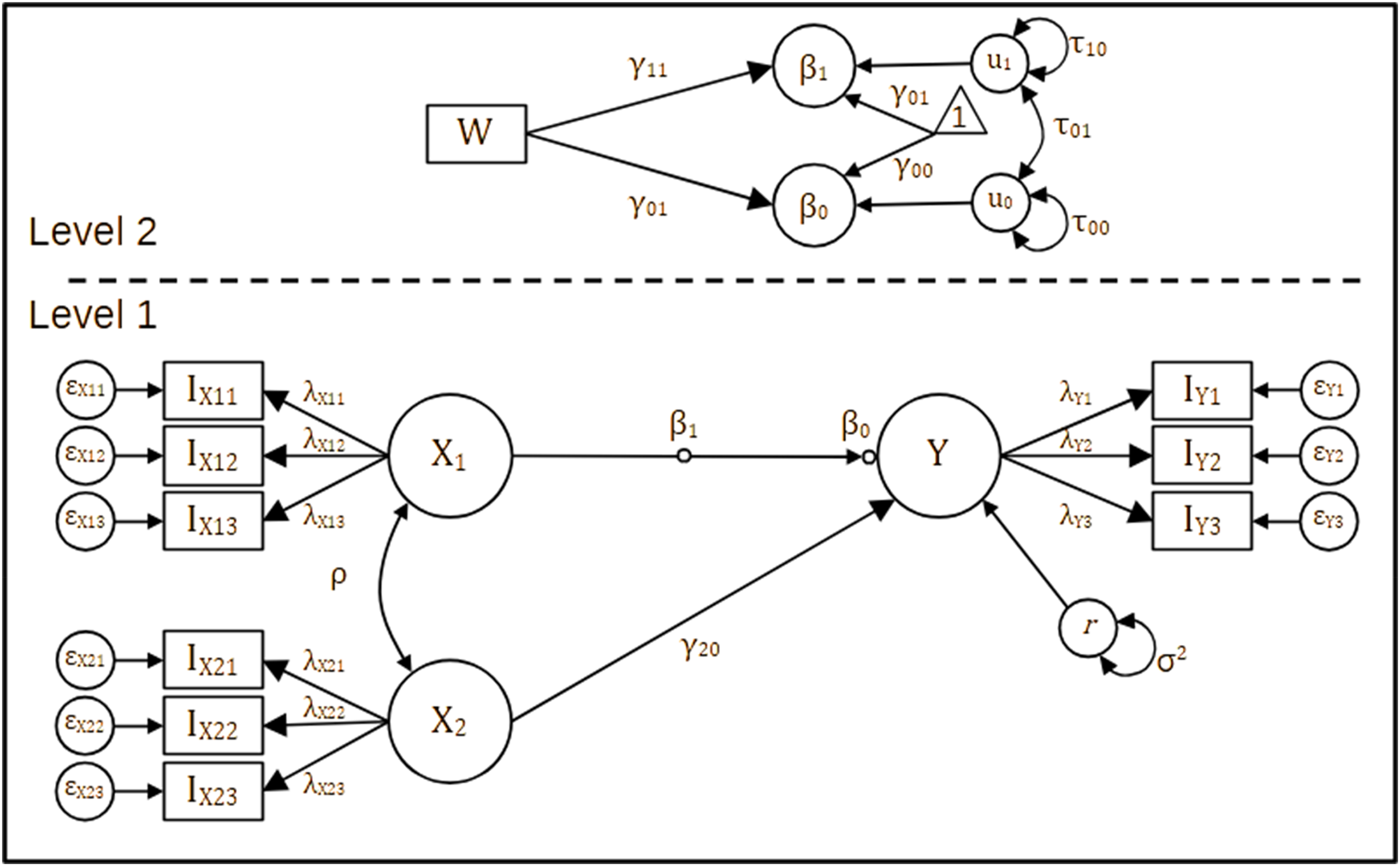
MM in an SEM framework where three latent variables of interest are each measured by a set of three indicators on the individual level (the lower part of the figure) with one manifest variable on the group level (the upper part of the figure), affecting both the random intercept and the random slope. See Table 2 for a description. MM: multilevel modelling; SEM: structural equation modelling.

Table 2 lists and describes all population parameters used in the study. We chose moderate parameter sizes typically found in sociological research to serve as population values (see specification below). Specifically, we included four fixed effects (γ₁₀, γ₂₀, γ₀₁, γ₁₁) and three random effects (τ₀₀, τ₁₁, τ₀₁).

We chose the sizes of the population parameters to reflect realistic (i.e., not too strong) effect sizes for both fixed and random effects. Specifically, the fixed effects coefficients were set to an average absolute value of 0.24, reflecting the expected population-level relationships between variables. For the random effects, the variance of the random intercept was set to 0.09 (standard deviation of 0.3, units of Y), and the variance of the random slope was set to 0.04 (standard deviation of 0.2, units of Y/X). The correlation between the random intercept and the random slope was specified as 0.15 (see Table 2). This approach was adopted to facilitate a realistic and balanced representation of both fixed and random effects in our simulations. In the measurement part of the model, we assumed linear relationships between latent variables and their indicators, characterized by two parameters: an intercept (μ) and an unstandardized loading (slope: λ).

The parameters of the structural model presented in Figure 1 are typically obtained using multilevel SEM with a maximum likelihood estimation (MLE) (Hox, Moerbeek, and van der Schoot 2018) or Bayesian estimation (Depaoli and Clifton 2015; Hox, Moerbeek, and van der Schoot 2018). Alternatively, researchers may employ composite scores as approximations for the values of the latent variables in standard MM regression. This approach is widely used by researchers (see Appendix 1 in the online Supplemental Material for more information); however, empirical analyses – and our findings below – demonstrate that this method leads to severely biased MM results (Devlieger and Rosseel 2020; see also Devlieger, Mayer, and Rosseel 2016; Lu et al. 2011, for similar results obtained in single-level settings). Other alternatives, such as MM factor score regression as proposed by Devlieger and Rosseel (2020) and the plausible values (PVs) method (Asparouhov and Muthén 2010), also have important limitations. The former, at least to date, does not enable the estimation of models with random slopes. The latter involves the generation of many sets of scores for each latent variable that must be analyzed separately, and the use of proper formulas to aggregate the results obtained by applying each set to obtain the final estimates. This procedure is burdensome, and the properties of the PV method for MM have yet to be studied.

This study focuses on three distinct scenarios. The first two involve the use of factor scores from a measurement model, either with full MI (scenario 1) or with varying degrees of MI violations (scenario 2). As previously noted, while the use of factor scores is prone to bias, it remains a common practice among applied researchers. The third scenario adheres to a more methodologically sound approach, utilizing multilevel SEM with MLE. Although less frequently utilized in applied research, this method is well-established and straightforward to implement with existing SEM software, such as Mplus (Muthén and Muthén 1998–2017). Prior studies have shown multilevel SEM to exhibit robust statistical properties in adequately large samples (cf. Heck and Thomas 2015; Hox, Moerbeek, and van der Schoot 2018).

Generating Latent Variables

We assumed that all individual-level variables (X₁, X₂, Y) were measured with measurement error using 3, 5, 10, 15, or 20 continuous indicators. In each iteration, the values of exogenous individual-level variables, X₁ and X₂, were sampled from a bivariate standard normal distribution, with a correlation between them set to 0.3. We independently sampled an exogenous group-level variable, W, from a standard normal distribution. Importantly, X₁ and X₂ were generated independently of the group structure. As a result, their group means were identical except for random variation, rendering them almost purely within-group variables. Consequently, X₁ and X₂ were nearly uncorrelated with the group-level variable W. While this setup may not reflect all situations encountered in real data or address every research question, it is consistent with the recommendation to use group-mean centred explanatory variables in MM (Enders and Tofighi 2007), particularly when the main substantive interest lies in estimating the within-group association between X and Y. Group-mean centring ensures that the level-1 predictors are uncorrelated with group-level variables, which facilitates the interpretation of within-group effects and avoids conflating them with between-group variation. Recognizing this aspect of our simulation design is crucial for interpreting the results, as it limits the propagation of bias in regression coefficients involving X₁ and X₂. In a way, this scenario represents a favourable situation: The impact of noninvariance on the coefficients will be greater when X₁ and X₂ contain substantial between-group variation.

Group-level random effects for the intercept and slope were sampled from a bivariate normal distribution, with expected values set to 0, standard deviations set to 0.3 and 0.2, respectively, and a correlation set to 0.15 (see Table 2). The individual-level error term for Y (r_ij) was generated from a normal distribution with an expected value of 0 and a variance (σ²) of 0.586, ensuring a standard normal distribution of Y.

Finally, values of the dependent latent variable Y were calculated according to Equation 6, based on the previously sampled values of the variables X₁, X₂, W, random effects, individual-level error terms, and the parameter values specified in Table 2. The resulting intraclass correlation coefficient (ICC) of Y at X₁ = 0 was 0.18 (it is important to note, however, that in the random slope model, the ICC is not constant but varies with X₁). Values generated in the population model were subsequently treated as known representations of latent constructs during the generation of observed indicators.

Introducing Measurement Noninvariance

As a starting point, the unstandardized factor loadings in the measurement part of the model were set to 1 for all observed indicators of X₁, X₂, and Y, while error term variances were fixed at 1 (corresponding to a standardized factor loading of about 0.707), and measurement intercepts were set to 0. To evaluate the impact of measurement noninvariance, we created several conditions. In the scalar equivalence condition, factor loadings and item intercepts were identical across all groups in the dataset, fixed at the values specified above. In the other conditions, we introduced variation in factor loadings and/or intercepts to simulate measurement noninvariance. Specifically, two medium-sized noninvariance conditions were implemented, where unstandardized factor loadings and intercepts deviated by 0.3 and 0.6, respectively, from the specified values in some groups. Similar deviations have been employed in other studies (Kim et al. 2017; Kim and Yoon 2011; Kim, Yoon, and Lee 2012; Meade and Lautenschlager 2004; Pokropek, Davidov, and Schmidt 2019; Shi, Song, and Lewis 2019), providing a robust foundation for examining our MI considerations. To reflect realistic situations, the sign (direction) of noninvariance was chosen randomly and independently for each measurement parameter. Noninvariant parameters were computed by adding (or subtracting, depending on the sampled sign of effect) noninvariance (to 25%, 50%, 75%, or 100% of the groups) to the default values specified in Table 2. Different sets of observed indicator parameters used in the simulations, depending on the conditions, are summarized in Table 3. We examined different types and intensities of noninvariance in the data, which were characterized by five factors:

Variables affected by noninvariance: dependent variable only (Y), independent variables only (X₁ and X₂), or both dependent and independent variables (X₁, X_2, and Y) (3 conditions)

Share of groups affected by noninvariance: 25%, 50%, 75%, or 100% (4 conditions)

Number of noninvariant indicators: 1/3 or 2/3 (2 conditions)

Size of noninvariance effect: 0.3 or 0.6 (2 conditions)

Level of invariance present: scalar, metric, or configural (3 conditions)

Table 3.

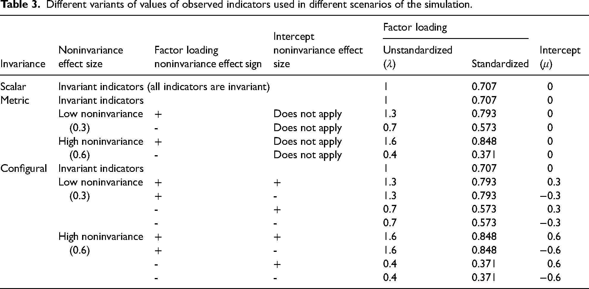
Different variants of values of observed indicators used in different scenarios of the simulation.

Invariance	Noninvariance effect size	Factor loading noninvariance effect sign	Intercept noninvariance effect size	Factor loading		Intercept (μ)
				Unstandardized (λ)	Standardized
Scalar	Invariant indicators (all indicators are invariant)			1	0.707	0
Metric	Invariant indicators			1	0.707	0
	Low noninvariance (0.3)	+	Does not apply	1.3	0.793	0
		-	Does not apply	0.7	0.573	0
	High noninvariance (0.6)	+	Does not apply	1.6	0.848	0
		-	Does not apply	0.4	0.371	0
Configural	Invariant indicators			1	0.707	0
	Low noninvariance (0.3)	+	+	1.3	0.793	0.3
		+	-	1.3	0.793	−0.3
		-	+	0.7	0.573	0.3
		-	-	0.7	0.573	−0.3
	High noninvariance (0.6)	+	+	1.6	0.848	0.6
		+	-	1.6	0.848	−0.6
		-	+	0.4	0.371	0.6
		-	-	0.4	0.371	−0.6

When interpreting the results, it is important to note that we maintained configural invariance across all simulated conditions. This means that the overall factor structure – the observed indicators and latent constructs – was identical across groups. While the constructs themselves were identical between groups, we manipulated MI by allowing certain items to differ in their factor loadings (metric noninvariance) or in both factor loadings and intercepts (scalar noninvariance) across groups. As a result, although the underlying constructs were consistent across groups and measured by the same items, some items became incomparable across countries due to intentional noninvariance.

For the data generation process, we utilized a self-developed R package multilevInv, employing the mnormt package (version 2.0.2; Azzalini and Genz 2020) to sample data from multivariate normal distributions and then the MplusAutomation package (Hallquist and Wiley 2018) to perform model estimation in Mplus. All simulation codes and results are publicly available in the Zenodo repository (multilevInv package: https://doi.org/10.5281/zenodo.16797849; the generated data and code used to perform the analyses: https://doi.org/10.5281/zenodo.16811563).

Generating Observed Indicators

When analyzing the accuracy of MM regressions (as opposed to multilevel SEM), the model relies on factor scores instead of latent variables. These factor scores were obtained using the software package Mplus 8.0 (Muthén and Muthén 1998–2017) based on two specifications: (1) single-group CFAs for the latent independent variables and (2) multigroup CFAs (i.e., MGCFAs) that assume full MI while allowing the means and variances of the dependent latent variables to vary across groups. Prior to estimating the MM regressions, the factor scores were standardized to have a mean of 0 and a standard deviation of 1 across the entire generated dataset. The resulting factor scores were obtained with varying numbers of observed indicators for each construct, with reliability estimates as follows: Three indicators resulted in a reliability of 0.750, 5 indicators had a reliability of 0.833, 10 indicators had a reliability of 0.909, 15 indicators had a reliability of 0.938, and 20 indicators had a reliability of 0.952.

Sample Sizes

For the datasets sampled from this population, we adopted conditions that typically apply to international survey data, which frequently serve as the basis for MM. Within-group sample sizes in international comparative surveys tend to exhibit limited variation. For example, the ESS requires a sample size of at least 1500 per country, the samples in the ISSP vary between 1000 and 1400, the WVS targets 1200 respondents per country, and the Eurobarometer requires at least 1000 respondents in each country sample. However, greater heterogeneity is observed in the number of groups across surveys in international comparative research. Depending on the survey round, Eurobarometer studies range from 13 to 39 countries, the ESS includes between 22 and 31 countries, and the ISSP covers between 7 and 37 countries. Some surveys involve even larger numbers of groups. For instance, the PISA survey includes up to 72 countries, the WVS collects data from five continents, and the Gallup Global Wellbeing study collects data from 155 countries. For our simulation study, we focused on conditions that apply to many of the surveys mentioned above, using datasets with 20 and 40 groups (i.e., countries) and with a sample size of 1000 in each group. Research by Meuleman and Billiet (2009) and Heisig, Schaeffer, and Giesecke (2017) indicates that 20 groups are desirable for running MM regressions, while 40 groups are recommended for multilevel SEM. Although Elff et al. (2020) suggested that fewer than 20 groups may be sufficient for MM regressions, our study concentrated on SEM. Therefore, we adhered to a minimum of 20 groups in our simulations.

The simulation resulted in a total of 194 distinct simulation conditions. Of these, 192 conditions stemmed from a fully crossed design involving six factors: 2 levels of invariance type (configural vs. metric), three variables affected, four levels of the share of groups affected, two levels of the number of items affected, two levels of the size of noninvariance, and 2 group sizes (20 vs. 40). In addition, two scalar invariance conditions (for 20 and 40 groups) were included as reference points. For the first two scenarios in which factor scores were used, we generated 1000 datasets per condition. For the multilevel SEM scenario, we randomly generated 400 datasets per condition (194 conditions) following the specifications detailed earlier. While 400 replications may appear modest, previous successful simulation studies involving complex models such as ours have employed even fewer replications. For instance, when analyzing models similar to ours, studies by Nylund, Asparouhov, and Muthén (2007), Meade and Lautenschlager (2004), and Kim et al. (2017) each used 100 replications per condition. In the two scenarios utilizing factor scores, we created 1000 datasets for each condition. Detailed Monte Carlo error estimates are provided in the online Supplemental Material Appendices 2, 3, and 4; they are consistently small, reinforcing the robustness and reliability of our study's findings.

Estimation Procedures

For the scenario where multilevel SEM is applied (scenario 3), we estimated the model depicted in Figure 1 using Mplus 8.0 software. We employed MLE with robust standard errors and the standard numerical integration method with 10 integration points. All other settings were kept at the Mplus defaults, including a maximum of 500 iterations and a convergence criterion of 0.000001.

It is important to note that this model operated under the assumption of an identical measurement model across groups, thereby overlooking the presence of noninvariance in the generated data. This allowed us to determine whether the model could still accurately retrieve the true population parameters.

The MM using factor scores in the first two scenarios were estimated using the lmer() function from the R package lme4 (Bates et al. 2015) with the restricted maximum likelihood (REML) criterion. We obtained 95% confidence intervals (CIs) for the estimated random parameters by profiling (restricted) likelihood using the lme4 function profile(). For the fixed effects parameters, we computed CIs using a t-distribution approximation with Satterthwaite's approximation for degrees of freedom, utilizing the R package lmerTest (Kuznetsova, Brockhoff, and Christensen 2017). Because the results of both approaches were very close, we focused our discussion on the profiled CIs.

Different estimation methods were employed for multilevel SEM and MM with factor scores, as the aim was not to directly compare estimates across frameworks. Each method was chosen as optimal for its respective modelling context, and this distinction does not compromise the validity of our conclusions.

Performance Measures of Parameter Recovery

To investigate the performance of MM under different conditions of MI in the second and third scenarios, we evaluated the relative parameter bias and the unbiased 95% CI coverage (the results for root-mean-square error are also presented in the online Supplemental Material Appendices 2, 3, and 4). Relative bias is presented in terms of percentages, that is, the average percentage of over- or under-estimation of the parameter of interest. It was calculated by dividing the bias by the true value of the parameter used during data generation. A relative parameter bias exceeding 10% was considered problematic. Thus, unbiased 95% CI coverage is a percentage of how many times the true value of the parameter falls within the bounds of the estimated 95% CI shifted by the value of the bias of this parameter (as estimated in this simulation). Ideally, this percentage should be as close as possible to its theoretical value of 95%. Deviations from this indicate standard error estimation inaccuracies: Coverage above 95% suggests overestimation, while coverage below 95% indicates underestimation. We considered coverage values close to 100% and below 90% as problematic because they would not allow for correct statistical inference at the assumed significance level.

Results

MM Regression Using Factor Scores: The Problem of Measurement Error

This section presents results for MM based on factor scores derived from varying numbers of indicators, ranging from 3 to 20 as per the conditions described above, with reliabilities ranging between 0.75 and 0.952, respectively. Note that measurement noninvariance has not been included in this analysis; instead, the focus is on the impact of using factor scores that neglect the presence of random measurement errors in the indicators. Only the two conditions in which scalar invariance is not violated are analyzed here. Figure 2 depicts the relative biases for: (1) Individual-level fixed effects in equations that include group-level effects (γ₁₀); (2) individual-level fixed effects in equations without group-level effects (γ₂₀); (3) group-level fixed effects on the intercept (γ₀₁); (4) group-level fixed effects on the slope (i.e., cross-level interactions); (5) random intercepts and (6) random slopes. For correlations between the exogenous latent variables and between random effects, results are briefly summarized as they are typically of less substantive interest in MM.

Figure 2.

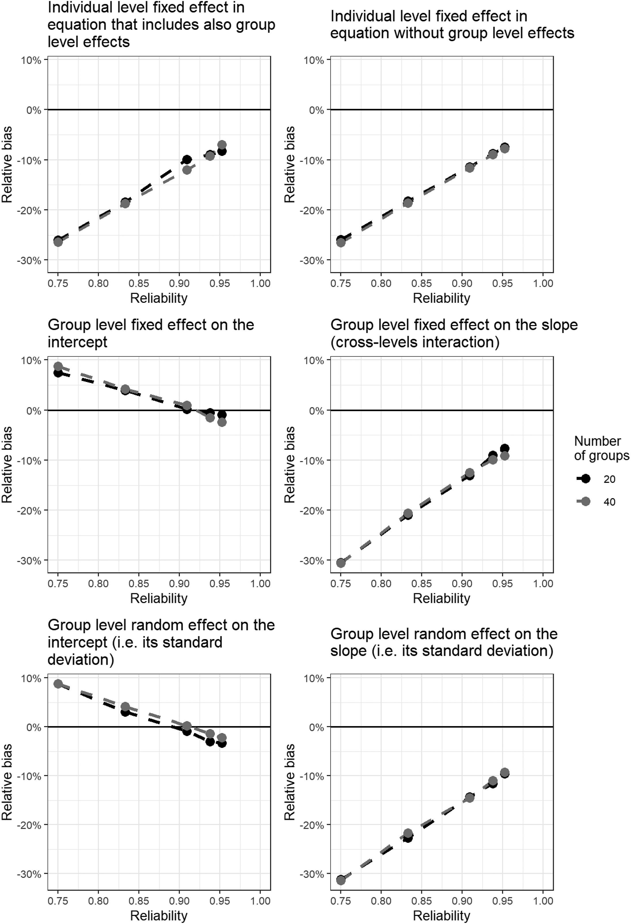
MM regression using factor scores with MI given. The relative bias of different MM parameters with different reliability of measurement. MM: multilevel modelling; MI: measurement invariance.

The analysis reveals that measurement error in independent variables leads to attenuation bias in MM, a well-documented phenomenon in regression analysis (Duncan 1975; Kenny 1979; Pokropek 2015). Specifically, individual-level fixed effects, cross-level interaction effects, and random slope effects consistently show a negative bias that intensifies as indicator reliability decreases. For example, with three items, 0.75 reliability, and 20 groups, the relative bias for the individual fixed effect parameter (γ₁₀) was −26.1%. With five items, 0.83 reliability, and 20 groups, the relative bias for γ₁₀ decreased to 18.4%. Keeping the number of groups constant at 20, further decreases of the parameter bias were observed if the number of indicators and the reliability increase: −9.9% for 10 items (0.91 reliability), −8.9% for 15 items (0.94 reliability), and −8.3% for 20 items (0.95 reliability).

This linear relationship between reliability and downward bias mirrors the attenuation effect found in ordinary least squares (OLSs) regression when predictors are measured with error. However, unlike OLS regression – where bias approaches zero as reliability nears one – our multilevel model indicates that small downward biases persist even at high reliability levels.

At the group level, both the fixed effect and the random effect for the intercept were substantially upward biased under conditions of lower reliability (the lowest reliability considered here being 0.75). The relationship between bias and reliability was again linear and negative. However, as reliability approached 1, the bias did not approach 0. Instead, at high reliability levels (e.g., 0.92), the bias became negative and became increasingly negative as reliability increased.

The bias pattern for the group-level fixed intercept (γ₀₁) is not universal. Its direction depends on how measurement error distorts the partitioning of variance between and within groups, which in turn is a function of the signs and magnitudes of the underlying within-level slopes. With the present parameterisation, attenuation of X₁ and X₂ reduces the within-group component of Y, inflating the apparent between-group mean difference and yielding a positive bias at low reliability. As reliability rises, the attenuation subsides and the intercept bias converges to zero, slightly overshooting into the negative. Alternative sign constellations for γ₁₀ and γ₂₀ would reverse this pattern. Hence, we treat this bias as design-specific rather than directionally systematic.

The number of groups had either a very minimal or no clear effect on group-level fixed effects or the random intercept. The CI coverage analysis (Appendix 2 in the online Supplemental Material) showed that, except for the individual-level fixed effect for X₂, parameter coverage approached nominal values as reliability increased. With only three or five items per construct, coverage was unacceptably low. Notably, coverage for the individual-level fixed effect for X₂ (i.e., for the variable not involved in group-level interactions) remained extremely low. Even at a reliability of 0.95, coverage did not exceed 20%, indicating substantial model limitations due to both parameter bias and underestimation of the model parameter standard error (the latter is supported by the considerable undercoverage of unbiased CIs – see Appendix 2 in the online Supplemental Material). In contrast, coverage of unbiased CIs for group-level fixed effects and the random intercept was consistently robust regardless of reliability, likely because group-level predictors were measured without error.

Our findings highlight that factor scores constructed from low-reliability indicators and ignoring random measurement errors can lead to substantial biases and inference errors in MM. To ensure that the results do not lead to erroneous conclusions, indicator reliability should ideally exceed 0.90, and preferably reach at least 0.94, which is unrealistically high for many applied studies. Notably, in our conditions, this was achieved only when using 15 items, corresponding to a reliability of 0.938. In the next part of our study, we examine the additional impact of measurement noninvariance on the results. To discern the independent role of measurement noninvariance, we focus on scenarios with sufficient reliability, that is, with 15 indicators and a reliability of 0.930.

MM Regression Using Factor Scores: The Problem of MI

This section investigates the effects of ignoring measurement noninvariance when applying MM regression with factor scores rather than modelling latent variables directly. Figure 3 illustrates the impact of measurement noninvariance across various conditions for relative bias and unbiased 95% CI coverage. The figure summarizes how different levels and types of noninvariance affect key model parameters, focusing on both individual- and group-level fixed and random effects. All results presented in Figure 3 refer to the condition with 15 indicators (thus, very high reliability) to avoid the substantial biases caused by measurement error in MM regression, as documented in the previous section. Results presented here are averaged across simulation conditions with 20 and 40 groups, as the differences between group sizes were negligible. Detailed results by group size are available in Appendix 3 in the online Supplemental Material.

Figure 3.

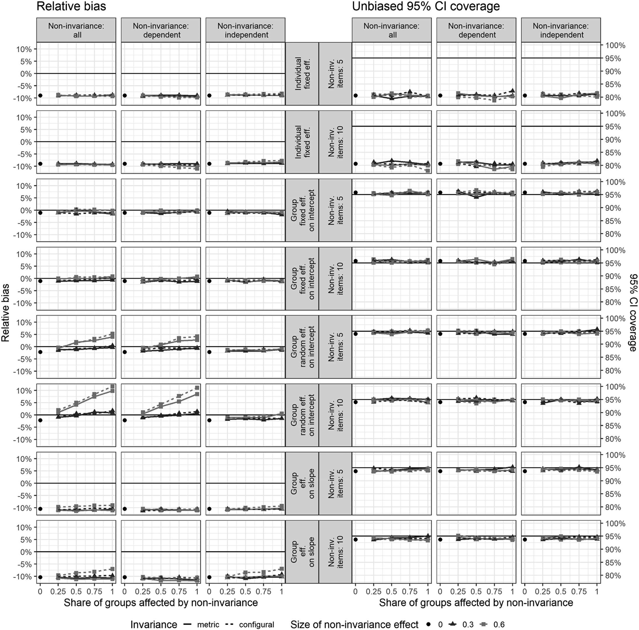
MM regression: Average relative bias and unbiased 95% CI coverage for different types of effects, averaged across conditions with 20 and 40 groups. MM: multilevel modelling; CI: confidence interval.

The left panel of Figure 3 illustrates the relative bias observed under the different noninvariance conditions: noninvariance of both the dependent and independent variables, noninvariance of only the dependent variable, and noninvariance of only the independent variables. Each row represents different parameter effects within the model: individual-level fixed effects (γ₁₀ and γ₂₀), group-level fixed effects (γ₀₁ and γ₁₁), group-level random effects on the intercept ( $\sqrt{{\tau }_{00}}$ ), and group-level random effects on the slope ( $\sqrt{{\tau }_{11}}$ ). The right panel of the figure focuses on the coverage of the unbiased 95% CIs under the same noninvariance conditions.

For individual-level fixed effects, noninvariance results in a bias of approximately −10% across all levels of noninvariance, with no significant variation between conditions. Even with larger noninvariance effects (0.6), the bias does not exceed this threshold. Regarding the estimates of parameter standard errors, the situation is more complex than suggested in Figure 3 (see Appendix 3 in the online Supplemental Material). Specifically, coverage of unbiased 95% CIs is very good for the variable involved in cross-level interactions (X₁), but reaches only about 65% for the variable not involved in the cross-level interaction (X₂). For both variables, these results are stable across conditions with varying intensities of noninvariance.

Noninvariance did not impact the group fixed effect on the intercept, with biases consistently close to zero across all conditions and unbiased 95% CI coverage almost perfectly aligning with the desired 95%. This result is not surprising, given that W is a manifest variable not affected by measurement noninvariance nor by measurement error in our simulation, and considering that X₁ and X₂ are predominantly within-group variables, uncorrelated with W.

The results for the standard deviation of group-level random effects on the intercept ( $\sqrt{{\tau }_{00}}$ ) clearly showed that noninvariance of the dependent variable introduced an upward bias in the size of the random effect for the intercept. In contrast, noninvariance of the independent variables appeared to have no significant effect. When the size of the noninvariance was small, the resulting bias remained minimal and did not fluctuate significantly when varying the level of noninvariance (metric or scalar) or the number of affected groups and items. However, under conditions of large (metric or scalar) noninvariance, the bias increased substantially with a growing number of affected groups and items. When the number of affected groups was large, the random effect for the intercept showed an upward bias of up to 10%. Nevertheless, parameter uncertainty was consistently estimated accurately across all conditions, as indicated by the coverage of unbiased CIs remaining very close to the nominal 95% rate.

The results for the standard deviation of the random slope ( $\sqrt{{\tau }_{11}}$ ) showed a consistent downward bias of approximately 10%, and this was independent of the investigated conditions. Interestingly, in conditions with high levels of MI and large numbers of groups and items, the bias tended to decrease from −10% to −5%, most likely due to the fact that, by chance, biases regarding MI and reliability cancelled each other out. Also, this parameter demonstrated very good coverage of the unbiased 95% CIs.

In sum, the simulation results indicate that measurement noninvariance may cause some bias in MM when factor scores are used, yet the primary source of bias remains the random measurement error in the indicators (as discussed in the previous section). Notable exceptions were observed for the group-level random effects of the intercept, where larger biases due to measurement noninvariance were evident.

Multilevel SEM: The Problem of MI

In the final set of simulations, we explored the effect of noninvariance when multilevel SEM is applied, using latent variables instead of factor scores. Unlike the high reliability conditions analyzed in the previous section, this analysis focuses on a more realistic scenario with only three indicators and moderate reliability (0.75). After all, multilevel SEM is effective in tackling the bias resulting from random measurement errors (Bollen 1989; Hox, Moerbeek, and van der Schoot 2018). Recall that under such conditions, MM regression based on observed scores led to significant bias in the estimates for most MM parameters due to measurement error, with CIs that often failed to cover the true values. While we know that SEM methodology effectively accounts for measurement error, it raises a key question: How does multilevel SEM perform when faced with MI bias? Is it, like standard MM, largely unaffected by noninvariance? It is important to note that the differences in biases between Figures 3 and 4 are not directly comparable as measures of model performance. The MM results in Figure 3 reflect high reliability conditions, while the multilevel SEM results in Figure 4 are based on models with fewer indicators.

Figure 4.

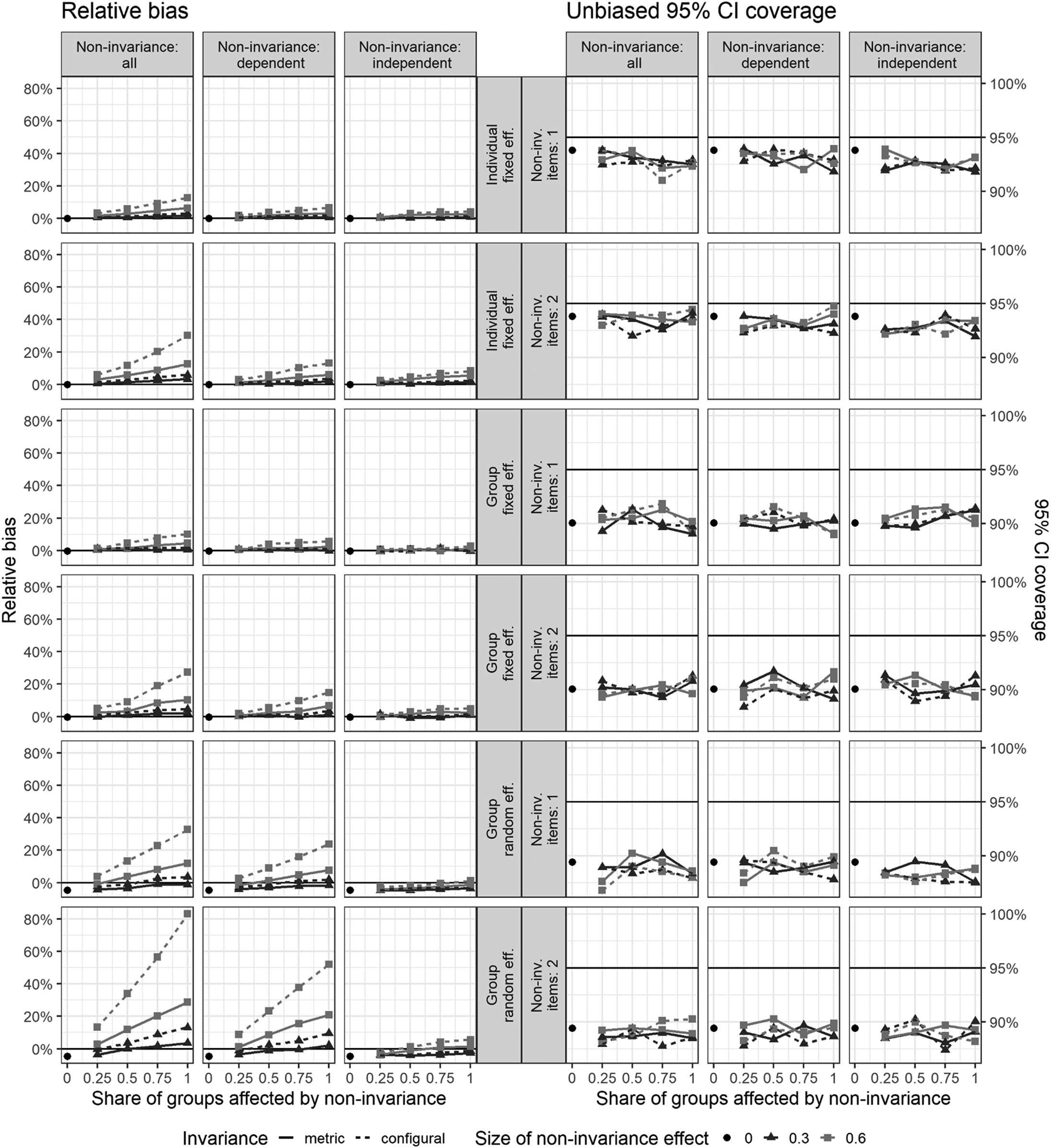
Multilevel SEM: Average relative bias and unbiased 95% CI coverage for different types of effects, averaged across conditions with 20 and 40 groups. SEM: structural equation modelling; CI: confidence interval.

Figure 4 illustrates the impact of measurement noninvariance on relative bias and unbiased 95% CI coverage across various model parameters, including fixed and random effects at both the individual and group levels. The plots are organized to display the influence of varying shares of groups affected by noninvariance under three conditions: ‘Noninvariance of both the dependent and independent variables’, ‘Noninvariance of only the dependent variable’, and ‘Noninvariance of only the independent variable’. The results are further categorized by the number of noninvariant items (1 or 2) and the size of the noninvariance effect (0, 0.3, 0.6), with black circles representing the absence of noninvariance. Results presented here are averaged across simulation conditions with 20 and 40 groups, as the differences between group sizes were negligible. Detailed results by group size are available in Appendix 4 in the online Supplemental Material.

When noninvariance is moderate (0.3), the relative bias in individual-level fixed effects is relatively small, generally below 10% across most scenarios. However, as the number of noninvariant items increases and the noninvariance effect size grows, the bias rises significantly. Noninvariance of the dependent variable consistently results in larger biases than noninvariance in the independent variables. The worst-case scenario – where both the dependent and independent variables are noninvariant across many items and groups – results in average effect parameter biases reaching as high as 35%. The cumulative nature of the bias is evident: the more groups and items affected by noninvariance, and the larger the noninvariance effect, the greater the bias. These findings highlight the importance of addressing noninvariance to avoid inflated parameter estimates in multilevel SEM models.

On the other hand, the coverage of unbiased CIs is somewhat lower than the nominal 95% rate, indicating that the standard errors of the parameters are slightly underestimated. This underestimation appears unrelated to the intensity of the noninvariance in specific simulation conditions. Two factors likely compound this under-coverage. First, multilevel SEM is estimated via full maximum likelihood, with no REML estimation method available, whereas in observed-variables MM, REML is known to yield more accurate sampling distributions for variance components (Elff et al., 2020). Second, the CIs were constructed in a typical way, assuming asymptotic normality; yet with only 20–40 groups, the sampling distribution of the group-level fixed-effect estimators is closer to a t-distribution with limited degrees of freedom, again producing too-narrow intervals. We checked the consequences of using a t distribution for the construction of CIs for these parameters. Using a simple rule of approximating the number of degrees of freedom for the t distribution (as advocated by i.e., Elff et al., 2020): m - l - 1, where m is a number of groups and l a number of group-level variables in a regression equation leads to widening CIs by about 7.2% and 3.3% in the 20 groups and 40 groups scenarios, respectively. This, in turn, enables the reduction of undercoverage of group-level fixed effects roughly to the level observed for the individual-level fixed effects (in Figure 4).

The group-level fixed effects parameters exhibited a similar behaviour to that of the individual-level fixed effects. As the number of affected groups and noninvariant items increased, the bias in the estimation of group-level fixed effects steadily grew. When at least half of the items were noninvariant, the bias remained relatively small because the remaining invariant items still contributed sufficient information to estimate the latent variables accurately at the group level. However, under more adverse conditions – when most items were noninvariant – the bias increased significantly, reaching as high as 35%.

This substantial bias occurred because measurement noninvariance at the group level resulted in inconsistent estimation of the latent dependent variable Y across groups. Since Y is measured differently in different groups due to noninvariant items, the group-level fixed effects that rely on Y become biased. Additionally, because X₁ and X₂ are predominantly within-group variables and are nearly uncorrelated with the group-level variable W, they were unable to mitigate this bias.

Moreover, extensive measurement of noninvariance in both the dependent variable Y and other variables amplified the bias in the group-level effects due to the additive effects of noninvariance across multiple variables. The coverage of the unbiased CIs showed that standard errors of group-level fixed effects were also underestimated, irrespective of the degree of noninvariance. However, the 95% unbiased CIs only covered the true values about 90% of the time on average, indicating a more substantial issue here compared to the individual-level fixed effects.

The lower parts of Figure 4 focus on the group-level random effects, specifically the standard deviation of the random intercept ( $\sqrt{{\tau }_{00}}$ ) and the random slope ( $\sqrt{{\tau }_{11}}$ ). These parameters were found to be highly sensitive to measurement noninvariance in terms of bias. As with other types of parameters, estimates of parameter standard errors were consistently deflated, with the coverage of the unbiased 95% CIs averaging slightly below 90%.

In general, random effect estimates exhibited an upward bias when noninvariance was present, with the magnitude of the bias increasing as the noninvariance effect size grew. When noninvariance was moderate (0.3), the relative bias for these random effects remained manageable, typically under 15%. However, under more severe noninvariance conditions (0.6), the bias could become substantial, reaching as high as 70–80% in extreme cases.

The bias was most pronounced when noninvariance affected both the dependent and independent variables. Specifically, the random intercept was more affected by noninvariance in the dependent variable alone, whereas the random slope exhibited greater sensitivity when both the dependent and independent variables were noninvariant (see Appendix 4 in the online Supplemental Material). In contrast, when only the independent variable was noninvariant, the bias of the random intercept was smaller and more stable, often below 20%, regardless of the number of groups or items affected.

With respect to parameter standard error estimates, unbiased 95% CIs showed, irrespective of the intensity of noninvariance, a consistent underestimation: minimal underestimation for individual-level fixed effects, more pronounced for group-level fixed effects, and most substantial for group-level random effects. Importantly, a detailed analysis (see Appendix 4 in the online Supplemental Material) indicated that this deflation of standard errors is considerably stronger in conditions with 20 groups but diminished in conditions with 40 groups. This finding underscores the importance of including a large number of groups in multilevel SEM analyses to ensure valid statistical inference, particularly when MI is not given.

Correlations between exogenous latent variables and random effects are generally of lesser interest. For detailed results, please see Appendix 4 in the online Supplemental Material. Briefly, correlation estimates between random effects were most impacted by noninvariance in the dependent variable, exhibiting severe upward bias, up to 200% under high noninvariance and up to 46% under low noninvariance. When metric invariance held, bias remained below 20%. Standard errors were consistently underestimated, especially in scenarios involving fewer groups.

Note that the biases observed in our analyses (especially, but not exclusively, for random effects) were consistently positive. This positive bias in coefficient estimates was primarily due to the overestimation of random effects in situations of measurement noninvariance. When MI was violated, the model encountered additional variation in parameters that was not accounted for, leading to an inflated estimation of random effects. Violations of MI introduced group-specific measurement error, which inflated the estimated variance of random effects (Jak, Oort, and Dolan 2013). This inflated random effects variance indirectly affected the fixed effects estimation due to the interconnected nature of variance components and fixed effects in multilevel models (Raudenbush and Bryk 2002). Specifically, when between-group variance was artificially inflated by MI violations, the model misattributed some of the measurement bias to true between-group differences. This misattribution distorted the weighting of within-group and between-group information, resulting in biased fixed effects estimates. This ‘spillover’ effect occurred because the estimation of fixed effects relies on accurately partitioning variance into within-group and between-group components. Consequently, violations of MI can have a cascading effect on parameter estimates throughout the model, distorting both random and fixed effects. Crucially, this mechanism operates even when the true within- and between-group effects are identical. Non-invariant indicators inflate the apparent between-group variance of the latent constructs; the model then absorbs this spurious variance into the random intercepts and slopes, altering the Empirical-Bayes shrinkage weights and pushing the fixed-effect estimates upward.

Conclusions, Discussion, and Recommendations for Researchers

This study provides a comprehensive investigation into the implications of measurement noninvariance and measurement error in MM through extensive Monte Carlo simulations. Our findings offer critical insights into how these factors bias results in MM.

First, our study demonstrates that failing to control for random measurement errors by using factor scores instead of latent variables may lead to severe bias in MM. The results unambiguously indicate that only exceptionally high (and uncommon in survey research) reliability – ideally surpassing 0.94 – can effectively mitigate the measurement error bias and inaccuracies introduced into MM by measurement errors. This requirement for high reliability presents a significant challenge in the realm of sociological cross-country comparisons. In this domain, the number of indicators used is typically limited, making it difficult to attain the level of reliability necessary to offset the effects of measurement error bias. However, the recently developed structural after measurement (SAM) approach proposed by Rosseel and Loh (2022) offers a promising solution. SAM employs Croon's measurement error corrected factor scores (Croon 2002; Devlieger, Mayer, and Rosseel 2016) and can be applied to multilevel structural models, especially in studies with small or medium sample sizes (Kelcey, Cox, and Dong 2021).

Second, our simulations revealed that while the presence of measurement noninvariance can introduce bias in MM estimates, its impact is generally less than traditional MM methods may produce results comparable to multilevel SEM, with only slightly greater bias than the bias resulting from measurement error. In particular, scenarios where measurement error is not adequately controlled exhibit more pronounced bias in MM than those influenced by noninvariance alone. Our findings demonstrate that when reliability is high (exceeding 0.93) or when a large number of indicators are used (15 in our simulations), measurement noninvariance did not introduce any critical bias in MM when factor scores are employed. This highlights the critical importance of considering measurement error in MM, particularly when factor scores are used in lieu of latent variables.

Third, our findings indicate that measurement noninvariance affects parameters only in cases of extensive MI violations and does not significantly influence CI coverage. Fixed effects proved to be particularly robust in high-reliability conditions. For random effects, small noninvariance introduced a minimal bias, especially when a large number of items and groups were involved. This is an encouraging result for researchers dealing with high-reliability data with a large number of indicators, but also highlights the challenges in sociological research, where the number of indicators is often limited.

Fourth, when used in conditions of complete MI, multilevel SEM, which controls for measurement errors, provides excellent results, as previous studies have demonstrated. However, our study revealed that in the absence of MI, even this advanced approach can produce quite biased results when reliability is low and MI affects many indicators across multiple groups. Despite these limitations, it is important to emphasize that multilevel SEM still performs significantly better than regular MM because it effectively controls for measurement error.

It is important to underscore that when reliability is high and the number of items is large, the advantage of using multilevel SEM compared to MM regression is relatively small. However, such conditions are rare in practice, and in most cases, sociologists are confronted with a small number of indicators with limited reliability. Yet the use of multilevel SEM is not a panacea. While our findings show that bias from lack of MI is smaller than from ignoring measurement error, it can still be substantial under specific conditions. Thus, testing for and establishing MI should precede MM analysis. Confidence in MM results can only be justified for indicators that have successfully passed MI testing.

As with all simulation-based studies, our research has limitations, primarily in the scope of conditions it could address. We recognize that it was not feasible to include every possible condition in our simulations. One notable limitation is that the variable X₁ was modelled with both a cross-level interaction and a random slope. This dual inclusion makes it challenging to disentangle the individual consequences of the cross-level interaction and the random slope on the observed estimation bias. While this model specification reflects common practice in MM, it does complicate the interpretation of results. Future research could address this by examining models in which these components are manipulated independently. Such an approach could help isolate their specific effects on parameter estimation and provide more nuanced guidance for practitioners.

Consequently, the results presented here should be interpreted as general guidance rather than strict, universally applicable rules. Each research context might present unique challenges and conditions that were beyond the scope of our study, and thus provide ample impetus for further research.

Practical Guidance for Researchers

Our study highlights the importance of incorporating best practices in MM, particularly regarding the reliability of indicators and MI. Based on our Monte Carlo simulations, we propose a structured approach to guide researchers in implementing MM and multilevel SEM.

The first step in any multilevel analysis should be assessing the reliability of the indicators used to measure the latent constructs. The reliability of the indicators reflects the consistency and accuracy of the measurements, playing a critical role in determining the appropriate modelling approach. If the reliability is high, that is, exceeds 0.94 – a threshold rarely achieved in typical survey research – then using traditional MM regression may suffice, as the risk of bias from measurement error is minimal. However, researchers should still exercise caution, as only exceptionally high reliability levels can ensure unbiased results.

When reliability falls below this threshold, which is more common in practice, the potential for bias increases significantly. In such cases, multilevel SEM is recommended, as it explicitly accounts for measurement error by modelling the relationships between latent variables and their observed indicators. Multilevel SEM can provide more accurate parameter estimates and reduce the impact of measurement error, especially when the reliability of the indicators is below the optimal threshold.

The next crucial step involves testing for MI. Ensuring that the measurement properties of the indicators are equivalent across groups is essential for valid cross-group comparisons. Researchers should follow established practices for testing MI, sequentially checking for configural, metric, and scalar invariance. If full MI is achieved, researchers can proceed with multilevel SEM. However, when full invariance is not met, researchers should consider adopting a partial invariance approach. This involves relaxing the equality constraints for parameters that exhibit noninvariance, while maintaining equality for the rest. Thus, to determine the appropriate approach, it is important to assess how many indicators and groups exhibit noninvariance.

Our study suggests that when noninvariance affects only a small number of groups and indicators, researchers can still use multilevel SEM while releasing the unequal slopes or intercepts. Valid results can be obtained by adopting partial invariance techniques that allow the noninvariant indicators to differ while constraining the invariant indicators. The simulations suggest that the introduced bias is likely to be minimal. For instance, if fewer than 25% of the groups or only one out of three indicators display noninvariance, the impact on parameter estimates is likely to be minor. Researchers can use model modification indices to identify the noninvariant intercepts and/or slopes and release them.

However, if noninvariance affects a large number of groups or indicators, even multilevel SEM may fail to produce unbiased results. Fortunately, more sophisticated approaches exist that enable multilevel analysis, even in situations of severe MI. For such scenarios, we recommend considering alternative modelling techniques capable of handling the complexity introduced by widespread noninvariance. These techniques include: (1) Multilevel SEM with multiple group analysis, an approach that allows researchers to test and account for measurement differences across groups by estimating separate parameters for each group (see Pokropek, Davidov, and Schmidt 2019, for an overview); (2) Bayesian multilevel SEM approaches which incorporate prior information about parameter distributions, thus helping to stabilize estimates in the presence of widespread noninvariance (Van Erp and Browne 2021); or (3) latent class models for MI which use a mixture modelling approach to identify subgroups within the data that exhibit different patterns of MI (Kim et al. 2016).

In sum, our findings highlight the importance of caution when measurement error is not accounted for and MI is not established. They also emphasize that multilevel SEM may not always outperform MM when reliability is exceptionally high and a large number of indicators are used. Under these ideal conditions, traditional MM methods may produce results comparable to multilevel SEM, with only slightly greater bias. However, such ideal conditions are rare in sociological, psychological, and educational research. In typical scenarios, where the number of indicators is limited and reliability is moderate, multilevel SEM remains the preferred choice for reducing bias and ensuring the accuracy of parameter estimates.

Supplemental Material

sj-docx-1-smr-10.1177_00491241251379459 - Supplemental material for Challenges in Multilevel Modelling: Cross-Group Measurement Noninvariance and Measurement Errors. A Monte Carlo Simulation Study

Supplemental material, sj-docx-1-smr-10.1177_00491241251379459 for Challenges in Multilevel Modelling: Cross-Group Measurement Noninvariance and Measurement Errors. A Monte Carlo Simulation Study by Artur Pokropek, Tomasz Żółtak, Eldad Davidov, Bart Meuleman and Peter Schmidt in Sociological Methods & Research

Supplemental Material

sj-pdf-2-smr-10.1177_00491241251379459 - Supplemental material for Challenges in Multilevel Modelling: Cross-Group Measurement Noninvariance and Measurement Errors. A Monte Carlo Simulation Study

Supplemental material, sj-pdf-2-smr-10.1177_00491241251379459 for Challenges in Multilevel Modelling: Cross-Group Measurement Noninvariance and Measurement Errors. A Monte Carlo Simulation Study by Artur Pokropek, Tomasz Żółtak, Eldad Davidov, Bart Meuleman and Peter Schmidt in Sociological Methods & Research

Supplemental Material

sj-pdf-3-smr-10.1177_00491241251379459 - Supplemental material for Challenges in Multilevel Modelling: Cross-Group Measurement Noninvariance and Measurement Errors. A Monte Carlo Simulation Study

Supplemental material, sj-pdf-3-smr-10.1177_00491241251379459 for Challenges in Multilevel Modelling: Cross-Group Measurement Noninvariance and Measurement Errors. A Monte Carlo Simulation Study by Artur Pokropek, Tomasz Żółtak, Eldad Davidov, Bart Meuleman and Peter Schmidt in Sociological Methods & Research

Supplemental Material

sj-pdf-4-smr-10.1177_00491241251379459 - Supplemental material for Challenges in Multilevel Modelling: Cross-Group Measurement Noninvariance and Measurement Errors. A Monte Carlo Simulation Study

Supplemental material, sj-pdf-4-smr-10.1177_00491241251379459 for Challenges in Multilevel Modelling: Cross-Group Measurement Noninvariance and Measurement Errors. A Monte Carlo Simulation Study by Artur Pokropek, Tomasz Żółtak, Eldad Davidov, Bart Meuleman and Peter Schmidt in Sociological Methods & Research