Sage Journals: Discover world-class research

Abstract

The parametric g-formula can be used to estimate causal effects of time-varying exposures on observable outcomes. It resolves intermediate confounding in such settings by specifying several parametric models, one each for every time-varying variable, and by performing micro-simulations. However, its restriction to applications with observable outcomes limits its usability for social sciences where variables of interest are often unobservable constructs. In such cases, measurement models are needed. We propose a new approach utilizing bias-adjusted three-step latent Markov models (LMMs) within the parametric g-formula. LMMs estimate the probability of membership in an unobservable state conditional on observed indicator variables. By replacing the parametric models in the g-formula with LMMs, micro-simulations are performed as usual to estimate a causal effect of the time-varying exposure. We illustrate this new approach by estimating the average treatment effect of unemployment on several unobservable mental health states utilizing longitudinal data from the Longitudinal Internet studies for the Social Sciences panel.

Keywords

causal inference latent variable models g-formula mental health unemployment

Introduction

Most research questions in the field of social and behavioral sciences, as well as health research, are causal. However, inferring causality from data is no straightforward task. The causal inference literature has identified several assumptions under which causal claims are valid. Most notably, exchangeability, positivity, consistency, no interference, and temporal order of events are regarded as sufficient conditions to identify causal effects (Cole and Frangakis 2009). Methods that allow for estimating causal effects under these assumptions are being developed at a rapid pace. An easily overlooked prerequisite for inferring causality is valid measurement (VanderWeele 2022). In most settings, measurements contain noise, or the construct of interest is not directly observable but measured through several indicators as is often the case in social and behavioral sciences. In such instances, the use of measurement models is required. However, the use of measurement models in causal inference has only recently gained attention (Bray et al. 2019; Clouth et al. 2022; Clouth, Pauws, and Vermunt 2023; Fish and Leite 2024; Lanza, Coffman, and Xu 2013; VanderWeele 2022) and respective methods are still underdeveloped. In this study, we present an analysis strategy for using latent Markov models (LMMs; Bartolucci, Farcomeni, and Pennoni 2013; Collins and Lanza 2010; Vermunt, Langeheine, and Bockenholt 1999; Wiggins 1955) to estimate causal effects using the g-formula bridging the gap between causal inference and measurement theory.

Exchangeability can be achieved using randomized controlled trials. Observational data, however, is typically characterized by self-selection of participants into treatment groups (Hernán and Robins 2006). For instance considering the exposure “employment status,” we might observe participants self-selecting into employment and non-employment groups based on several confounding variables¹ such as age, gender, education, ethnicity, etc. (Bijlsma et al. 2017). If this is indeed the case, assigning an individual from the employment group to the non-employment group (and vice versa) would change the confounder distribution of these two exposure groups. That is, individuals from these groups are not exchangeable. To achieve exchangeability in this setting, the data requires manipulation. The literature on causal inference provides several methods for such manipulation of the data with regard to the variables influencing the self-selection, such as matching (Gu and Rosenbaum 1993) and inverse propensity weighting (IPW; Imbens 2000; Rosenbaum and Rubin 1983). Alternatively to these manipulation strategies, standardization (Hernán and Robins 2006) or its generalization, the g-formula (Robins 1986), can be used to estimate causal effects.²

While widely used in epidemiology and public health research, these methods are underutilized in the field of social and behavioral sciences. One reason for this might be that social and behavioral sciences often deal with constructs that are not directly observable (Bollen 2002). For instance, we might want to estimate the causal effect of employment status on mental health. Mental health, however, is an unobservable construct that can be operationalized in several ways. For instance, Bijlsma et al. (2017, 2019) investigated the effect of employment status on the outcome variable “first antidepressant purchase.” In the social and behavioral sciences, researchers often take a more direct approach by using patient reported outcome measures (see, for instance, Bubonya, Cobb-Clark, and Ribar 2019; Frijters, Johnston, and Shields 2014; Olesen et al. 2013). The outcome mental health might be regarded as a latent variable where indicators of that variable, such as ratings on the scales “I feel happy,” “I feel down,” “I feel tired,” can be directly observed. When choosing such a latent variable approach, the use of measurement models is required for which latent class analysis (LCA), a model-based clustering technique, can be used (Goodman 1974; Lazarsfeld and Henry 1968). LCA allows for estimating the relationship between the latent classes and auxiliary variables while accounting for the fact that the latent variable is measured imperfectly by the observed indicators. LCA has been extended for the longitudinal setting, that is, an LMM, otherwise known as hidden Markov model or latent transition analysis. With these models, a Markov chain is assumed where class membership is conditioned on class membership at the previous timepoint (additional to an individual's values on indicators and covariates).

Causal LCA and LMM have been proposed before. Lanza, Coffman, and Xu (2013), Clouth et al. (2022), and Clouth, Pauws, and Vermunt (2023) proposed different approaches for using IPW to estimate the causal effect of an exposure on class membership in a cross-sectional LCA. The approach by Lanza and colleagues was extended for longitudinal settings with multiple (time-constant) exposures (Bartolucci, Pennoni, and Vittadini 2016), time-varying exposures (Tullio and Bartolucci 2022), and time unobserved heterogeneity (Pennoni, Paas, and Bartolucci 2023). Recently, Bartolucci, Pennoni, and Vittadini (2023) proposed a new causal latent transition model inspired by a difference-in-differences approach (Imbens and Wooldridge 2009). However, these approaches rely on the assumption of no intermediate or post-treatment confounding.

Intermediate or post-treatment confounding occurs when time-varying confounders are affected by treatment or exposure at previous timepoints (Daniel et al. 2013; Robins 1986). For instance, additional to the time-constant confounders mentioned above, in our non-employment example, there are time-varying confounders such as income, household status, and physical health (Bijlsma et al. 2017, 2019). Job loss can lead to reduced physical health which, in turn, affects the propensity of employment at the following timepoint and, therefore, confounds the effect of non-employment on mental health at this following timepoint. If the outcome, in this case mental health, is also assessed repeatedly, there will also be intermediate confounding by the outcome. That is, mental health has an effect on the time-varying confounders and the propensity of employment which in turn confounds the effect of non-employment on mental health at the following timepoint. Figure 1 depicts these interrelationships in a directed acyclic graph (DAG) with the outcome “mental health” being depicted as the latent variable X measured by the observed indicators Y. The standard g-formula solves this issue of intermediate confounding by conditioning the outcome on the entire trajectory of exposures and confounders to estimate the causal effect of the time-varying exposure (Keil et al. 2014; Naimi, Cole, and Kennedy 2017; Robins 1986). The g-formula consists of several steps. First, a series of multivariable generalized linear models is estimated for each time-varying variable in our DAG. Next, we define the counterfactual scenarios of interest, that is, average mental health under exposure regimes “always employed” and “never employed.” Then, using the estimated multivariable models, we perform a series of simulations to obtain the outcome under each counterfactual scenario (Keil et al. 2014). The g-formula is a popular approach for estimating causal effects in the presence of time-varying confounding because the ATE can then simply be calculated as the marginal difference of these two counterfactuals.

Figure 1.

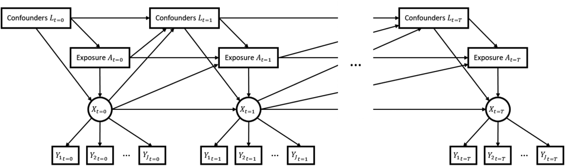
Directed acyclic graph (DAG) of the latent states–exposure–confounder relationship at timepoints $t = 0, \dots, T$ .

To identify the causal effect of non-employment on mental health where mental health is treated as a latent construct, we propose a new approach that utilizes an LMM within the g-formula. In detail, we propose the use of a bias-adjusted three-step LMM (Bartolucci, Montanari, and Pandolfi 2015; Di Mari, Oberski, and Vermunt 2016) in place of generalized linear models in the g-formula. LMMs can be described with two models, the measurement model and the structural model. In the measurement model, the relationship between the latent states and the observed indicator variables is estimated. In the structural model, the relationship between the latent states and other observed auxiliary variables is estimated. In a first step, we estimate the measurement part of the LMM which turns out to be a simple latent class model on the pooled data over all timepoints. In a second step, based on the obtained parameter estimates, individuals are classified into the latent classes (or states) at each timepoint, and classification errors are saved. In a third step, three types of structural models are estimated while accounting for the classification errors from step two. One structural model is required for estimating the relationship of the latent states over time (Markov chain) conditional on exposure and confounders. One structural model is required for the exposure as a distal outcome of state membership and confounders. One structural model is required for each confounder as a distal outcome of state membership and exposure. Defining the counterfactual scenarios of interest and performing the series of simulations for obtaining potential outcomes under the counterfactual scenarios can then be done as would be done if the outcome variable was directly observed.

The remainder of this article is structured as follows. In the second section, we provide a detailed description of our newly proposed approach of using an LMM within the g-formula. In the third section, we demonstrate this analysis strategy on data from the LISS (Longitudinal Internet studies for the Social Sciences) panel administered by Centerdata (Tilburg University, The Netherlands) including a detailed description of the step-by-step analysis strategy. We end with a discussion and conclusion section.

The Causal LMM

Causal Estimand for LMMs

Following work by Bartolucci, Pennoni, and Vittadini (2016) and Tullio and Bartolucci (2022), we reformulate the LMM in terms of the potential outcomes framework for defining the average treatment effect (ATE) as our estimands in LMMs. A detailed description of the parameterization and estimation of this ATE using LMMs is provided in the Section “The G-Formula for Latent Outcomes.”

Considering a structure as depicted in Figure 1, we define and identify the ATE at timepoint t as

\begin{matrix} A T E_{t} = P (X_{t}^{\bar{a} = \bar{1}}) - P (X_{t}^{\bar{a} = \bar{0}}) = P (X_{t} | \bar{A} = \bar{1}, L_{t}) - P (X_{t} | \bar{A} = \bar{0}, L_{t}) \end{matrix}

(1)

where

X_{t}

refers to a latent variable as opposed to an observed outcome variable at timepoint t,

\bar{A}

refers to an exposure level that is set to a particular value, and

L_{t}

refers to a set of observed confounding variables at timepoint t. Note that here, we define the potential outcomes for the ATEs under

\bar{a} = a_{0}, a_{1}, \dots, a_{t}

, hence, the full sequence of exposure over time rather than the exposure at a specific timepoint. Specifically, we define

\bar{a} = a_{0}, a_{1}, \dots, a_{t} = \bar{1}

and

\bar{a} = a_{0}, a_{1}, \dots, a_{t} = \bar{0}

corresponding to the hypothetical intervention scenarios “always exposed” and “never exposed”. Alternative definitions are possible.

The ATE as defined above is identified on the data under the assumptions of exchangeability, positivity, consistency, and no interference. In the case of an unobserved outcome that is modeled with an LMM, additional assumptions apply such as Markovianity, conditional independence, and stationarity (Bartolucci, Farcomeni, and Pennoni 2013). All assumptions applying to the causal LMM presented here are summarized in Table 1.

Table 1.

Assumptions Underlying the Causal Latent Markov Model.

Causal identification assumptions
(Conditional) Exchangeability or no confounding
Assumes that individuals from both exposure groups can be exchanged without influencing the outcome. In this study, exchangeability might be violated if individuals in the employed (exposed) group are more highly educated as exchanging those individuals for (lower educated) individuals from the non-employed (non-exposure) group could influence the latent outcome mental health. In this case, conditional exchangeability might still hold, for instance, if individuals from the employed group are exchanged with individuals from the non-employed group with the same educational level. In technical terms, if exchangeability holds, the counterfactual outcome is independent from the observed exposure level, i.e.,
$P (X_{a} = 1 \| A = 1) = P (X_{a} = 1 \| A = 0)$ and if conditional exchangeability holds, counterfactual outcome is independent from the observed exposure level conditional on the value of the confounding variable(s), i.e., $P (X_{a} = 1 \| A = 1, L) = P (X_{a} = 1 \| A = 0, L)$ .
Positivity
Assumes a non-zero probability of observing both exposure levels for all combinations of values on the confounding variables, i.e., $P (A = a \| L = l) > 0$ for all l with $P (L = l) \neq 0$ . If there exist combinations of confounders for which all individuals are either exposed or unexposed, it becomes unfeasible to estimate the ATE within these strata.
Consistency
This assumption connects observed outcomes with potential outcomes. Consistency assumes that for each individual, the outcome under the observed exposure is the same as if the exposure was hypothetically assigned. For this to be possible, the exposure must be well-defined, i.e., there cannot be multiple versions of the exposure. For the example in this study, consistency is likely violated as the exposure employment encompasses different types of jobs with different working hours. Estimates of the ATE should then be interpreted as average effects across these variations.
No interference
Assumes that an individual's potential outcomes are unaffected by the exposure assignments of the other individuals.

Assumptions related to the LMM
Markovianity
The latent state X at t depends solely on the latent state at $t - 1$ , i.e., $P (X_{t} = x_{t} \| X_{1 : t - 1} = x_{1 : t - 1}, Y_{1 : t - 1} = y_{1 : t - 1}) = P (X_{t} = x_{t} \| X_{t - 1} = x_{t - 1})$
Conditional independence
The observed indicator Y at t depends solely on the latent state X at t, i.e., $P (Y_{t} = y_{t} \| X_{1 : t - 1} = x_{1 : t - 1}, Y_{1 : t - 1} = y_{1 : t - 1}) = P (Y_{t} = y_{t} \| X_{t} = x_{t})$
Stationarity
The transition probabilities are time independent, i.e., $P (X_{t} = j \| X_{t - 1} = l) = P (X_{t + k} = j \| X_{t + k - 1} = l)$ , where $k = {0, \dots, t}$

Assumptions related to the parametric model specifications
Parametric homogeneity
The parameterization of the structural models is time independent, i.e., $P (X_{t} \| A_{t}, L_{t}) = P (X_{t + k} \| A_{t + k}, L_{t + k})$ and $E (L_{t} \| X_{t} A_{t}) = E (L_{t + k} \| X_{t + k} A_{t + k})$ , where $k = {0, \dots, t}$
Linearity
The parameterization of the structural models assumes a linear relationship between the (logit of) state membership, exposure level, and the confounders.

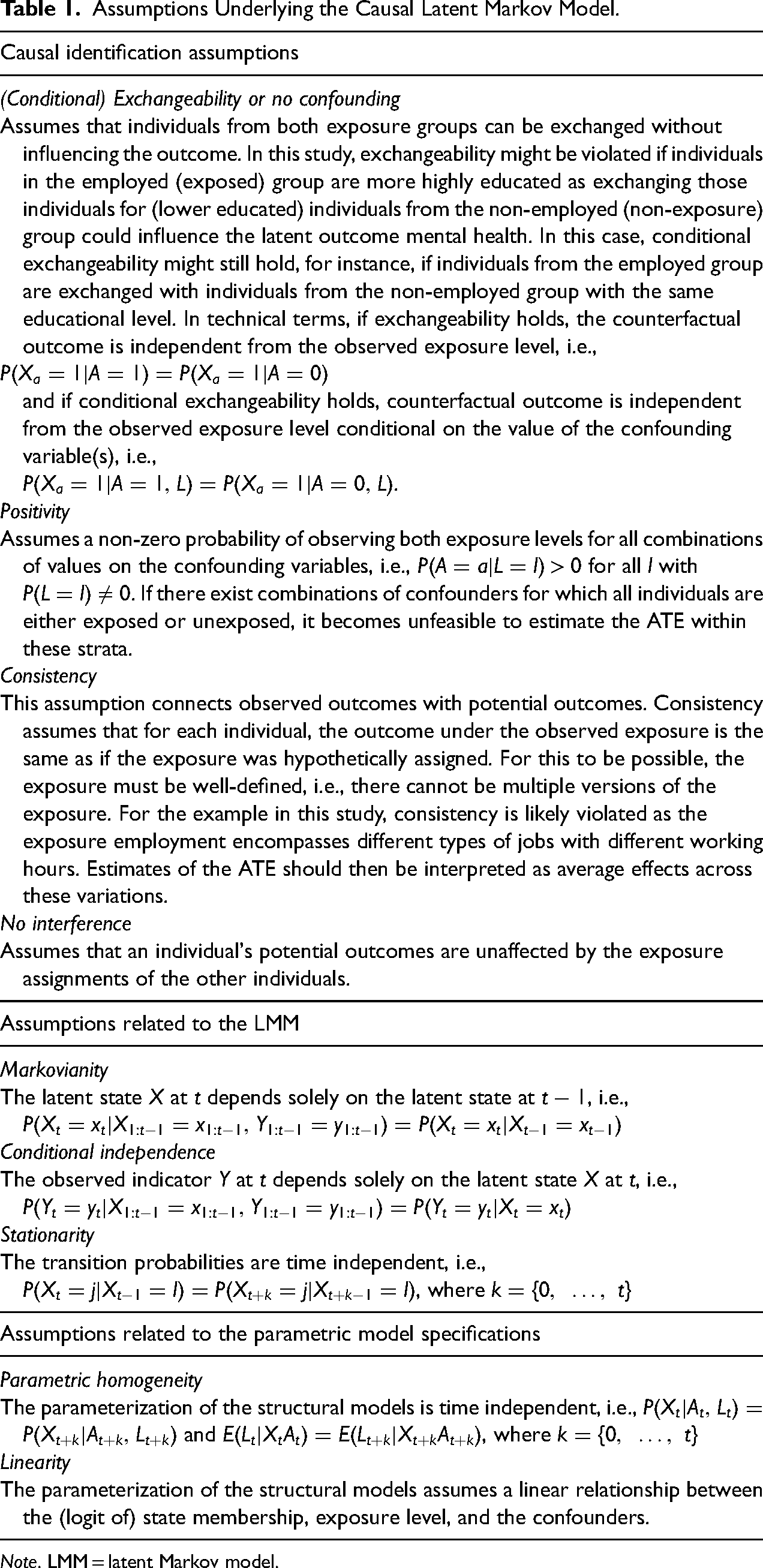
Note. LMM = latent Markov model.

The G-Formula for Latent Outcomes

Here, we utilize the g-formula to estimate the ATE of “always exposed” versus “never exposed” in the scenario as depicted in Figure 1. In detail, let us assume that for individual i, latent outcomes 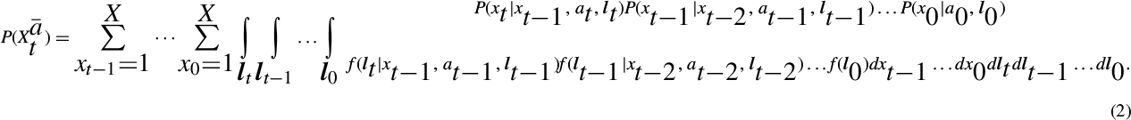$X_{i t}$ , exposures $A_{i t}$ , and confounders $L_{i t}$ are measured at time $t = 0, \dots, T$ . Naturally, the latent outcomes $X_{i t}$ are not directly observed but measured by indicators utilizing the LMM. Details of the LMM are presented in the section “The Bias-Adjusted Three-Step LMM.” As shown in Figure 1, we assume a Markov process where each variable at t is conditional on the values of that variable at $t - 1$ . Furthermore, the latent outcome $X_{i t}$ at t is conditional on exposure $A_{i t}$ and confounders $L_{i t}$ at t,³ exposure $A_{i t}$ at t is conditional on the confounders $L_{i t}$ at t and the latent outcome $X_{i t - 1}$ at $t - 1$ , and the confounders $L_{i t}$ at t are conditional on the outcome $Y_{i t - 1}$ and the exposure $A_{i t - 1}$ at $t - 1$ . $X_{i t}^{\bar{a}}$ then denotes the potential latent outcome of individual i at t with an exposure sequence of $\bar{A} = \bar{a}$ . In our example, $\bar{a}$ might refer to the sequence “always employed” or “never employed.” Under the identifying assumptions discussed above, the g-formula estimator of $E (X_{t}^{\bar{a}})$ at t is then

The ATE is then defined as the difference in latent outcomes under some hypothetical exposure regimes, that is, we might set 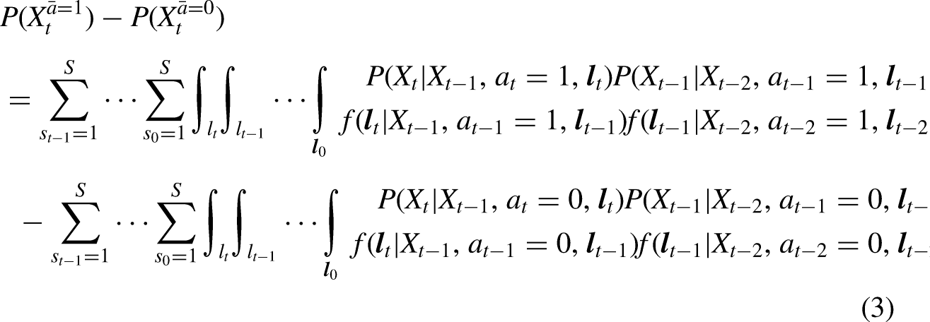$\bar{a} = a_{0}, \dots, a_{t - 1}, a_{t} = \bar{1}$ and $\bar{a} = a_{0}, \dots, a_{t - 1}, a_{t} = \bar{0}$ in equation (2) to estimate $E (X_{t}^{\bar{a} = \bar{1}}) - E (X_{t}^{\bar{a} = \bar{0}})$ . Note, that if the g-formula estimator of interest were $E (X_{t})$ , for instance because one might want to model the natural course, equation (2) needs to be adjusted to condition on the empirically observed distribution of $a_{t}$ . The g-formula estimator of $A T E_{t}$ as defined in equation (1) is then

\begin{aligned} P (X_{t}^{\bar{a} = 1}) - P (X_{t}^{\bar{a} = 0}) \\ = \sum_{s_{t - 1} = 1}^{S} \dots \sum_{s_{0} = 1}^{S} \int_{l_{t}} \int_{l_{t - 1}} \dots \int_{l_{0}} \begin{matrix} P (X_{t} | X_{t - 1}, a_{t} = 1, l_{t}) P (X_{t - 1} | X_{t - 2}, a_{t - 1} = 1, l_{t - 1}) \dots P (X_{0} | a_{0} = 1, l_{0}) \\ f (l_{t} | X_{t - 1}, a_{t - 1} = 1, l_{t - 1}) f (l_{t - 1} | X_{t - 2}, a_{t - 2} = 1, l_{t - 2}) \dots f (l_{0}) d l_{t} d l_{t - 1} \dots d l_{0} \end{matrix} \\ - \sum_{s_{t - 1} = 1}^{S} \dots \sum_{s_{0} = 1}^{S} \int_{l_{t}} \int_{l_{t - 1}} \dots \int_{l_{0}} \begin{matrix} P (X_{t} | X_{t - 1}, a_{t} = 0, l_{t}) P (X_{t - 1} | X_{t - 2}, a_{t - 1} = 0, l_{t - 1}) \dots P (X_{0} | a_{0} = 0, l_{0}) \\ f (l_{t} | X_{t - 1}, a_{t - 1} = 0, l_{t - 1}) f (l_{t - 1} | X_{t - 2}, a_{t - 2} = 0, l_{t - 2}) \dots f (l_{0}) d l_{t} d l_{t - 1} \dots d l_{0} \end{matrix} \end{aligned}

(3)

where

s_{t} = 1, \dots, S_{t}

refer to the states of the latent variable

X_{t}

at time t. As the expression in equation (2) cannot generally be evaluated analytically, the g-formula relies on Monte Carlo integration (Robins 1986). This procedure consists of the following steps.

(1) Models need to be specified and fit for each time-varying variable. Usually, generalized linear models are used in the g-formula but generally, there are no restrictions on what models can be implemented. For instance, here, we replace these generalized linear models with the structural models from bias-adjusted three-step LMMs. Note that these models are assuming a first-order Markov process, that is,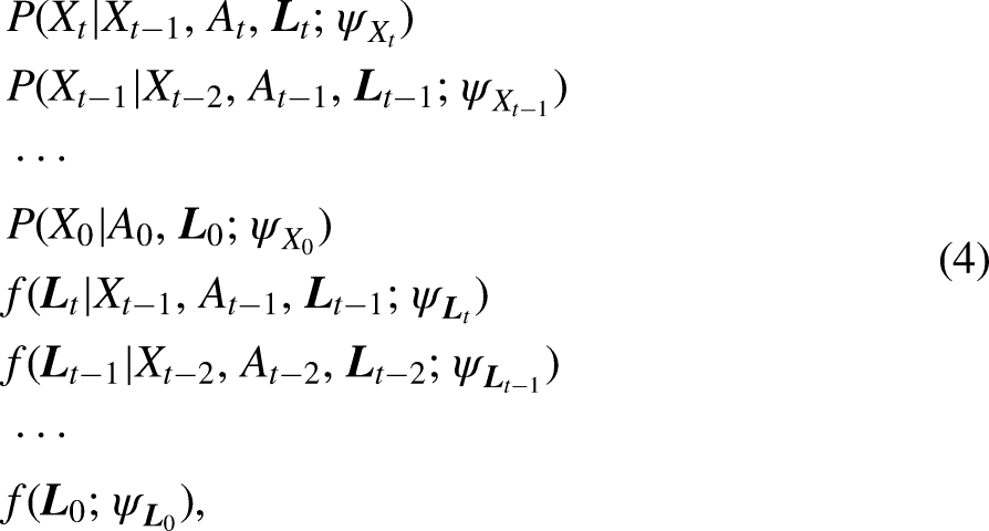

\begin{aligned} P (X_{t} | X_{t - 1}, A_{t}, L_{t}; ψ_{X_{t}}) \\ P (X_{t - 1} | X_{t - 2}, A_{t - 1}, L_{t - 1}; ψ_{X_{t - 1}}) \\ \dots \\ P (X_{0} | A_{0}, L_{0}; ψ_{X_{0}}) \\ f (L_{t} | X_{t - 1}, A_{t - 1}, L_{t - 1}; ψ_{L_{t}}) \\ f (L_{t - 1} | X_{t - 2}, A_{t - 2}, L_{t - 2}; ψ_{L_{t - 1}}) \\ \dots \\ f (L_{0}; ψ_{L_{0}}), \end{aligned}

(4)

with

ψ

representing the model parameter in question. However, alternative specifications with longer lags are possible. A model for the exposure is not required when the ATE is defined as the difference between two hypothetical scenarios. If, however, the ATE is defined as the difference between a hypothetical scenario and the natural course, that is, the average treatment effect on the treated (ATT), also a model for the exposure is required (Rudolph et al. 2022). Furthermore, one might want to compare the natural course to the original data to check for gross model misspecifications (Rudolph et al. 2022).

(2) Monte Carlo integration is used by simulating the longitudinal outcomes and confounders for each individual under each exposure scenario. Given the maximum likelihood estimators of the parameters 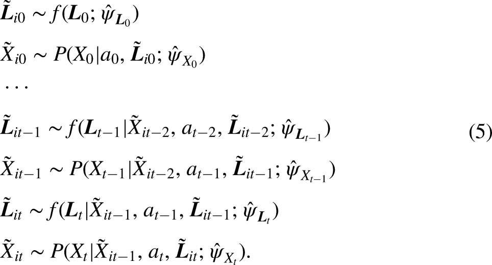$ψ$ , we sequentially simulate for each individual $i$ :

\begin{aligned} {\tilde{L}}_{i 0} \sim f (L_{0}; {\hat{ψ}}_{L_{0}}) \\ {\tilde{X}}_{i 0} \sim P (X_{0} | a_{0}, {\tilde{L}}_{i 0}; {\hat{ψ}}_{X_{0}}) \\ \dots \\ {\tilde{L}}_{i t - 1} \sim f (L_{t - 1} | {\tilde{X}}_{i t - 2}, a_{t - 2}, {\tilde{L}}_{i t - 2}; {\hat{ψ}}_{L_{t - 1}}) \\ {\tilde{X}}_{i t - 1} \sim P (X_{t - 1} | {\tilde{X}}_{i t - 2}, a_{t - 1}, {\tilde{L}}_{i t - 1}; {\hat{ψ}}_{X_{t - 1}}) \\ {\tilde{L}}_{i t} \sim f (L_{t} | {\tilde{X}}_{i t - 1}, a_{t - 1}, {\tilde{L}}_{i t - 1}; {\hat{ψ}}_{L_{t}}) \\ {\tilde{X}}_{i t} \sim P (X_{t} | {\tilde{X}}_{i t - 1}, a_{t}, {\tilde{L}}_{i t}; {\hat{ψ}}_{X_{t}}) . \end{aligned}

(5)

Note that instead of specifying a model for $f (L_{0}; ψ_{L_{0}})$ , ${\tilde{L}}_{i 0}$ can be drawn from the empirical distribution of $L_{0}$ or the empirical values of $L_{0}$ can be used directly (Bartlett, Olarte Parra, and Daniel 2023).

(3) Step (2) is repeated multiple times, that is, $r = 1, \dots, n_{syn}$ , to account for Monte Carlo error. The g-formula estimate for ${\tilde{X}}_{i t}$ is then obtained as $(1 / n_{syn}) \sum_{i = 1}^{n_{syn}} {\tilde{X}}_{i t}$ . Standard errors for $X_{t}$ can be obtained using non-parametric or parametric bootstrapping. Here, we use an alternative, computationally less intensive, quasi-Bayesian Monte Carlo method that involves sampling parameter sets directly from a multivariate normal distribution which is defined by the point estimates and the estimated asymptotic covariance matrix (Imai, Keele, and Tingley 2010; King, Tomz, and Wittenberg 2000; Vermunt and Magidson 2021b).

The Bias-Adjusted Three-Step LMM

To implement the g-formula when the outcome is not directly observed but measured through several indicators as depicted in Figure 1, a measurement model is needed for which we propose the use of a bias-adjusted three-step LMM (Di Mari, Oberski, and Vermunt 2016). The LMM consists of two parts, the measurement model and the structural model. In the measurement model, the relationship between the $j = 1, \dots, J$ observed indicators $Y_{t}$ and the $s_{t} = 1, \dots, S_{t}$ latent states $X_{t}$ at time $t = 0, \dots, T$ is defined. In the structural model, the relationship between the latent states $X_{t}$ and auxiliary variables, here, the exposure $A_{t}$ and confounders $L_{t}$ , as well as the relationship of the latent states $X_{t}$ over time is defined (Bartolucci, Montanari, and Pandolfi 2015; Collins and Lanza 2010; Di Mari, Oberski, and Vermunt 2016). To implement the g-formula with the LMM, we first estimate the measurement model and keep it fixed for the consecutive steps. Then, instead of specifying and fitting generalized linear models as described above, we specify and fit the structural models of the LMM, one structural model defining the relationship between the latent states $X_{t}$ with exposure $A_{t}$ and confounders $L_{t}$ as covariates and one structural model each for the confounders $L_{t}$ as distal outcome of the latent states and exposure $A_{t}$ .

In detail, the three steps of this approach of estimating the LMM are (1) estimating the measurement model, (2) classifying individuals into the latent states, and (3) estimating the structural model while accounting for the classification errors from step 2 (Bakk, Tekle, and Vermunt 2013; Di Mari, Oberski, and Vermunt 2016; Vermunt 2010):

(1) A latent class model without covariates is defined for each timepoint. We assume⁴ that this measurement model is the same at all timepoints and estimate it on the pooled observations where observed responses of the same individual at different timepoints are considered to be independent, that is, corresponding to different sample units. The model at each timepoint t is defined as:

\begin{matrix} P (Y = y) = \prod_{t = 0}^{T} \sum_{s = 1}^{S} P (X_{t} = s_{t}) P (Y_{t} = y_{t} | X_{t} = s_{t}) \end{matrix}

(6)

where

P (X_{t} = s_{t})

reflects the state proportions and

P (Y_{t} = y_{t} | X_{t} = s_{t})

the state-specific conditional response probabilities. As defined in equation (4), we assume conditional (or local) independence of the indicators, also with regard to covariates such that

\begin{matrix} P (Y_{t} = y_{t} | X_{t} = s_{t}) = \prod_{j = 1}^{J} P (Y_{j t} = y_{j t} | X_{t} = s_{t}) . \end{matrix}

(7)

This assumption could be easily relaxed by including direct effects between the indicators themselves or between the indicators and the covariates in the measurement part of the model (Vermunt and Magidson 2021a). The model is usually parameterized as logistic models and estimated by maximizing the log-likelihood function $L_{STEP 1} = \sum_{i = 1}^{n} \sum_{t = 0}^{T} \log P (Y_{i t} = y_{i t})$ .

(2) Next, the posterior state probabilities $P (X_{t} = s_{t} | Y_{t} = y_{t})$ are easily obtained from the probabilities in equation (4) by applying Bayes’ theorem. Individuals can then be assigned to state $W_{t}$ where the probability of the assigned state given the observations $P (W_{t} = s_{t} | Y_{t} = y_{t})$ depends on the assignment rule. With LMMs, modal assignment is commonly used where we allocate a weight $ω_{y t s} = P (W_{t} = s_{t} | Y_{t} = y_{t}) = 1$ if $P (X_{t} = s_{t} | Y_{t} = y_{t})$ is largest and zero otherwise. The classification errors, that is, the probability of state assignment conditional on the true state, $P (W_{t} = r_{t} | X_{t} = s_{t})$ with $r = 1, \dots, S$ can then be obtained as:

\begin{matrix} P (W_{t} = r_{t} | X_{t} = s_{t}) = \frac{[1 / (n (T + 1))] \sum_{i = 1}^{n} \sum_{t = 0}^{T} P (X_{t} = s_{t} | Y_{i t} = y_{i t}) ω_{i t r}}{P (X_{t} = s_{t})} . \end{matrix}

(8)

(3) In the last step, the relationship between the latent states and the exposure, confounders and previous latent states is estimated. For this, it is important to realize that the relationship between covariates and the assigned state memberships $P (W = r | A, L)$ and the relationship between covariates and true state memberships $P (X = s | A, L)$ are related as follows (Bolck, Croon, and Hagenaars 2004; Di Mari, Oberski, and Vermunt 2016; Vermunt 2010):

\begin{matrix} P (W = r | A, L) = \sum_{s_{0} = 1}^{S} \sum_{s_{1} = 1}^{S} \dots \sum_{s_{T} = 1}^{S} P (X_{0} = s_{0} | A_{0}, L_{0}) \prod_{t = 1}^{T} P (X_{t} = s_{t} | X_{t - 1} = s_{t - 1}, A_{t}, L_{t}) \prod_{t = 0}^{T} P (W_{t} = r_{t} | X_{t} = s_{t}) . \end{matrix}

(9)

The covariate-dependent initial state probabilities and transition probabilities can then be estimated by maximizing the following log-likelihood function: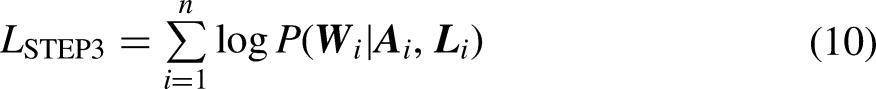

\begin{matrix} L_{STEP 3} = \sum_{i = 1}^{n} \log P (W_{i} | A_{i}, L_{i}) \end{matrix}

(10)

where

W_{t}

acts as a single indicator and the classification error probabilities

P (W_{t} | X_{t})

are treated as known.

Furthermore, if $L$ is regarded as a distal outcome rather than a covariate, $f (L | W, A)$ is related to $f (L | X, A)$ as:

\begin{matrix} f (L_{t} | W_{t - 1} = r_{t - 1}, A_{t - 1}) = \sum_{s = 1}^{S} f (L_{t} | X_{t - 1} = s_{t - 1}, A_{t - 1}, L_{t - 1}) P (W_{t - 1} = r_{t - 1} | X_{t - 1} = s_{t - 1}) \end{matrix}

(11)

and parameters can be estimated by maximizing

\begin{matrix} L_{STEP 3} = \sum_{i = 1}^{n} \log f (L_{i} | W_{i}, A_{i}) . \end{matrix}

(12)

Note that the log-likelihood function in equation (12) is maximized for each confounder L separately.

Real-Life Data Example

In this section, we illustrate our newly proposed analysis strategy to investigate the relationship between non-employment and mental health over time. Poor mental health and depression are leading contributors to the global burden of disease (Lepine and Briley 2011) and key factors of economical productivity (Layard 2013). Individuals with poor mental health show lower levels of economic activity, lower earnings, more difficulties in both finding and retaining employment, and reduced financial security (Bubonya, Cobb-Clark, and Ribar 2019). In turn, non-employment is associated with loss of workplace social contacts, time structures, and purposeful activity which can lead to reduced mental health (Jefferis et al. 2011). This temporal interplay has been studied before (for instance, see Bijlsma et al. 2017, 2019; Bubonya, Cobb-Clark, and Ribar 2019; Frijters, Johnston, and Shields 2014; Olesen et al. 2013; Steele, French, and Bartley 2013). In particular, Bijlsma et al. (2017, 2019) used the g-formula to account for the intermediate confounding that arises in this setting. However, the g-formula in combination with a latent variable model has not been used before to model the temporal interplay between non-employment and mental health.

Data

In this paper, we make use of data of the LISS panel administered by Centerdata (Tilburg University, The Netherlands). The LISS panel is a representative sample of Dutch individuals who participate in monthly internet surveys. The panel is based on a true probability sample of households drawn from the population register. Households that could not otherwise participate are provided with a computer and internet connection. A longitudinal survey is fielded in the panel every year, covering a large variety of domains including health, work, education, income, housing, time use, political views, values, and personality. More information about the LISS panel can be found at: www.lissdata.nl.

Here, we used five waves of the LISS core study with data being collected between 2017 and 2021. Participation rates varied between the waves and participants outside the labor force, that is, attending an educational program or being retired, were excluded. Not all individuals participated in all five waves used in this study. Missing values on the indicator variables are accounted for in the estimation of the LMMs using full information maximum likelihood estimation. This includes the missing information of participants that were not included in some of the waves. Observations for individuals with missing values on the exposure and confounders were imputed using MICE (Van Buuren and Groothuis-Oudshoorn 2011). As this article serves an educational purpose, we decided to only impute a single set and considered the data complete for demonstrating the use of the g-formula. Table OS1 (online Supplemental materials) summarizes descriptive statistics of all variables employed in this analysis. Detailed code including the imputation procedure is available on GitHub: https://github.com/felixclouth/Causal-inference-for-latent-Markov-models-using-the-parametric-G-formula (Clouth 2025).

Measures

Outcome

Defining the outcome and subsequently the ATE is not trivial when considering latent constructs. Here, we label the outcome as “mental health” and define it as latent states that manifest themselves in the observed indicators “I felt very anxious,” “I felt so down that nothing could cheer me up,” “I felt calm and peaceful,” “I felt depressed and gloomy,” and “I felt happy.” All items were scored on a six-point Likert scale ranging from “never” to “continuously.” Considering formula (7), $j = 1, \dots, 5$ refers to these indicators. For instance, $y_{i = 1, j = 1, t = 1}$ refers to the observed value of individual 1 on the indicator “I felt very anxious” at timepoint 1. While these five items do not provide a comprehensive measure of the construct “mental health,” they closely resemble in form a variety of items that are used in the literature, for example, items from the Short Form Health Survey (Ware et al. 2000). The final latent outcome is then the result of estimating the first step of the three-step LMM which is reported in the Results section. The ATE is then the marginal difference in membership probabilities for these states under “always employed” versus “never employed.”

Exposure

The exposure in our study is employment status coded as “being employed” versus “not being employed.” “Being employed” is defined as conducting work for pay, either as an employee, self-employed professional, or assisting in a family business. “Not being employed” is further defined as not conducting work for pay. This includes individuals who perform unpaid (voluntary) work or care and economically inactive individuals. Individuals who were too young to perform any work for pay or who attended an educational program and individuals who reached retirement age during the study period were excluded from the sample. Note that employment status might be considered to be a not well-defined exposure. “Employment” encompasses a variety of occupations with different salaries and working hours. Similarly, “non-employment” can refer to different situations such as job-seeking, performing unpaid work, or being economically inactive. The estimates of the ATEs present below should therefore be interpreted as average effects across these variations.

Confounders

We identified the following variables as time-constant confounders of the mental health—employment relationship. Age was recorded in years. Gender was recorded as “male” and “female.” Education was recorded as highest reached educational qualification. The categories “primary school,” “vmbo,” “havo/vwo,” “mbo,” “hbo,” and “wo” are specific to the Dutch educational system. “Vmbo” and “havo/vwo” are high school degrees, “mbo” refers to vocational training, and “hbo” and “wo” are university degrees. Origin was recorded as “no migration background,” “first generation western migration background,” “first generation non-western migration background,” “second generation western migration background,” and “second generation non-western migration background.” Additionally, the year of measurement was recorded.

Furthermore, we identified the following variables as time-varying confounders of the mental health—employment relationship. Subjective general physical health was recorded on a five-point Likert scale ranging from “poor” to “excellent.” Household status was recorded as “married,” “separated,” “divorced,” “widowed,” and “never been married.” Income was recorded as monthly gross household income in euros.

The list of confounding variables that were accounted for in this analysis is likely incomplete. Factors such as behavioral problems earlier in life, personality traits, or substance use have previously been identified as potential confounders of the employment–mental health relationship (Bijlsma et al. 2017). Causal interpretations of the results presented in this study thus need to be drawn cautiously.

Step-by-Step Analysis Strategy

Here, we describe in detail the algorithm for implementing the g-formula on the data from the LISS panel.

First, we estimate the measurement model (see equation (6)). Based on the pooled data over all timepoints, we estimate a latent class model without covariates using the observed indicators “I felt very anxious,” “I felt so down that nothing could cheer me up,” “I felt calm and peaceful,” “I felt depressed and gloomy,” and “I felt happy.” Performing LCA involves a model selection step. For this, several models are estimated with increasing number of latent classes. Among these candidate models, the model that fits the data best is selected. Model fit can be determined based on significance testing, such as the likelihood ratio test, information criteria, such as the Bayesian information criterion (BIC) or Akaike information criterion, or local fit indices, such as bivariate residuals. Subsequently, the local independence assumption might be relaxed by including direct effects between indicators to increase model fit. For this study, however, this was not necessary. After determining the final measurement model, individuals are classified into the latent states at each timepoint using modal assignment and classification errors are stored (see equation (8)).

Next, we estimate the structural models.

A multinomial logistic regression model is estimated for latent state X at t conditional on latent state X at $t - 1$ , employment status at t, the time-varying confounders physical health, income, and household status at t, and the time-constant confounders age, gender, education, origin, and year of measurement (see equation (10)).

A multinomial logistic regression model is estimated for physical health at t conditional on latent state X at $t - 1$ , employment status at $t - 1$ , physical health and the other time-varying confounders at $t - 1$ , and the time-constant confounders (see equation (12)).

A linear regression model is estimated for income at t conditional on latent state X at $t - 1$ , employment status at $t - 1$ , income and the other time-varying confounders at $t - 1$ , and the time-constant confounders (see equation (12)).

A multinomial logistic regression model is estimated for household status at t conditional on latent state X at $t - 1$ , employment status at $t - 1$ , household status and the other time-varying confounders at $t - 1$ , and the time-constant confounders (see equation (12)).

If the natural course scenario is of interest, also a logistic regression model is estimated for employment status at t conditional on latent state X at $t - 1$ , employment status at $t - 1$ , the time-varying confounders at t, and the time-constant confounders.

To be able to estimate standard errors for the ATE later, for every parameter estimate, we draw 500 values from the estimated parameter distribution. Alternatively, non-parametric bootstrap could be performed. Then, 500 samples would be drawn from the data and the structural models would be estimated on each sampled data set.

In the following, for each bootstrap sample, we perform a set of micro-simulations to generate the natural course scenario. A detailed description of this algorithm is provided in the online Supplemental materials. In short, we essentially follow the steps described in equation (5), however, now also including simulations of the exposure “employment status.” After simulating confounders, exposure, and outcome at the first timepoint as a function of its predictors, at each timepoint, we simulate these time-varying variables based on the simulations at previous timepoints. In order to minimize the Monte Carlo error, multiple draws, for example, 100, are taken and the probabilities for the outcome, that is, the state membership probabilities, are averaged over all random draws. The natural course scenario can then be compared to the empirical data to check for gross model misspecifications.

We repeat step 3, however, instead of simulating values for employment, we always set the value for employment to 1. This is the hypothetical intervention scenario of “always employed” (see first part of equation (3)).

We repeat step 3, however, instead of simulating values for employment, we always set the value for employment to 0. This is the hypothetical intervention scenario of “never employed” (see second part of equation (3)).

Next, the ATE is calculated by subtracting the state membership probabilities from the hypothetical intervention scenario of “never employed” from the state membership probabilities from the hypothetical intervention scenario of “always employed” (see equation (3)). Note that this calculation depends on the definition of the causal effect and other definitions of causal effects are possible.

If the quasi-Bayesian Monte Carlo method as described above was used in step 2, steps 3–6 are repeated for each sampled set and results are averaged over all the sampled ATEs. If non-parametric bootstrap was used, steps 2–6 are repeated for each bootstrap set and results are averaged over all the bootstrapped ATEs and standard errors for the ATE are obtained as the standard deviations across bootstrap replications.

Results

We identified three latent states based on the BIC, bivariate residuals (see Table 2), and interpretability of the latent states.⁵ The identified states are sufficiently separated with posterior state membership probabilities above .9 per classified state (see Table OS3 in the online Supplemental materials). Individuals in state 1 (44.5%) showed slightly elevated levels on all indicators and is labeled “slightly elevated mental health problems” (see Figure 2). Individuals in state 2 (37%) showed good to very good values on all indicators and is labeled “good mental health.” Note that for the indicators “feel calm” and “feel happy,” we inverted the scales so that low scores correspond to good values. Individuals in state 3 (18.5%) showed high values on all indicators and is labeled as “poor mental health.” In all three states, scores on the items “feel calm” and “feel happy” were slightly elevated. Furthermore, all three states show a similar structure in scores, however, on different levels, even though no modeling restrictions such as an ordinal scale for the latent variable were imposed.

Figure 2.

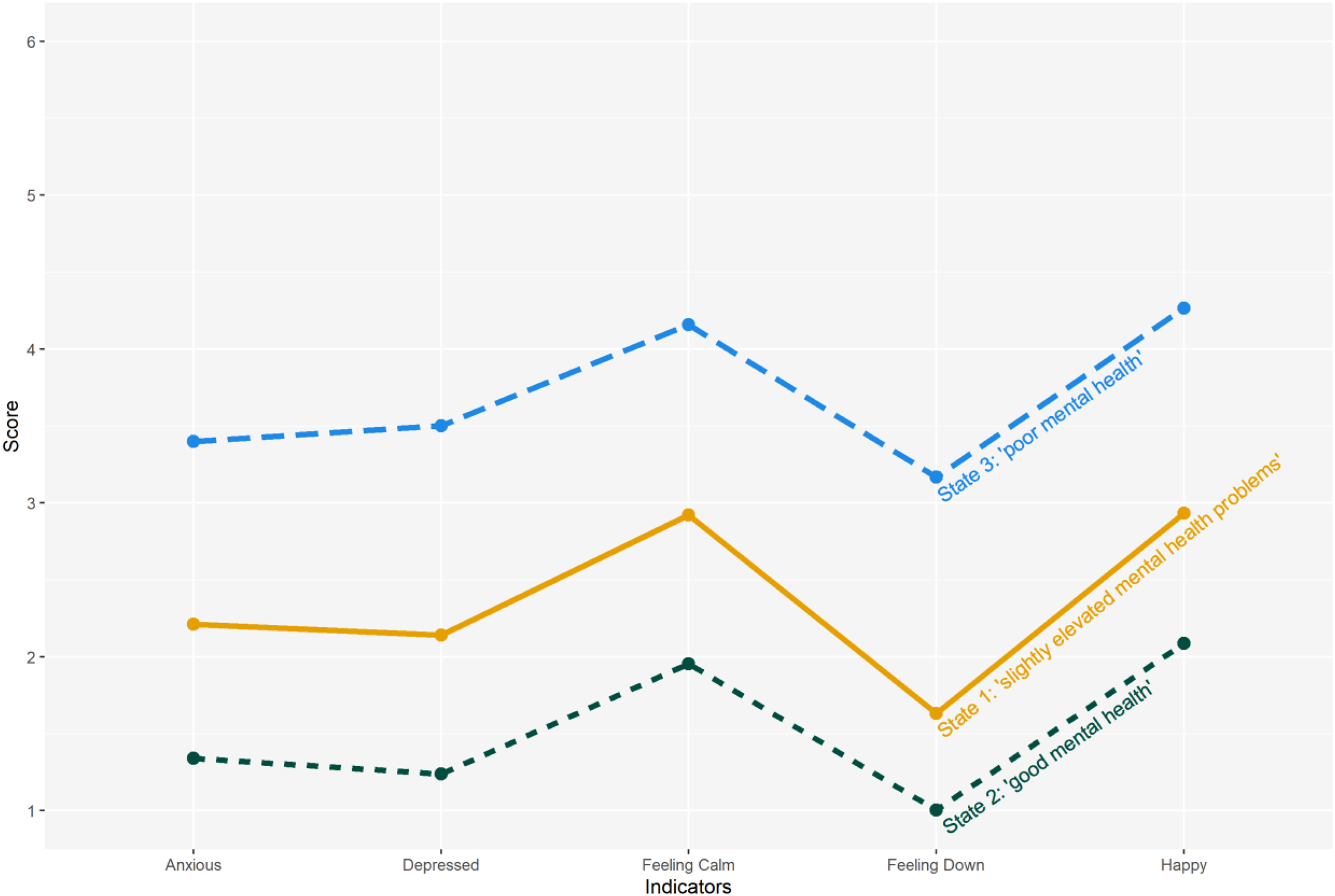
Composition of the latent states as estimated in step 1 of the bias-adjusted three-step LMM. Class-specific average scores are presented for all five observed indicators. Note that for the indicators “feel calm” and “feel happy,” the scales were inverted so that low scores correspond to good values. Note. LMM = latent Markov model.

Table 2.

Goodness of Fit Statistics. Log-Likelihood Values, Bayesian Information Criterion (BIC), Akaike Information Criterion (AIC), and Maximum Bivariate Residual (BVR) Values are Presented for Models with 1–5 States. The selected solution is highlighted in bold.

	Log-likelihood	BIC	AIC	Max. BVR
1 state	−101,776.0	203,802.2	203,601.1	15,264.3
2 states	−89,877.3	180,066.1	179,816.7	2,050.0
3 states	−86,689.4	173,750.4	173,452.7	773.0
4 states	−85,629.2	171,690.3	171,344.4	609.1
5 states	−84,678.8	169,849.8	169,455.6	428.2

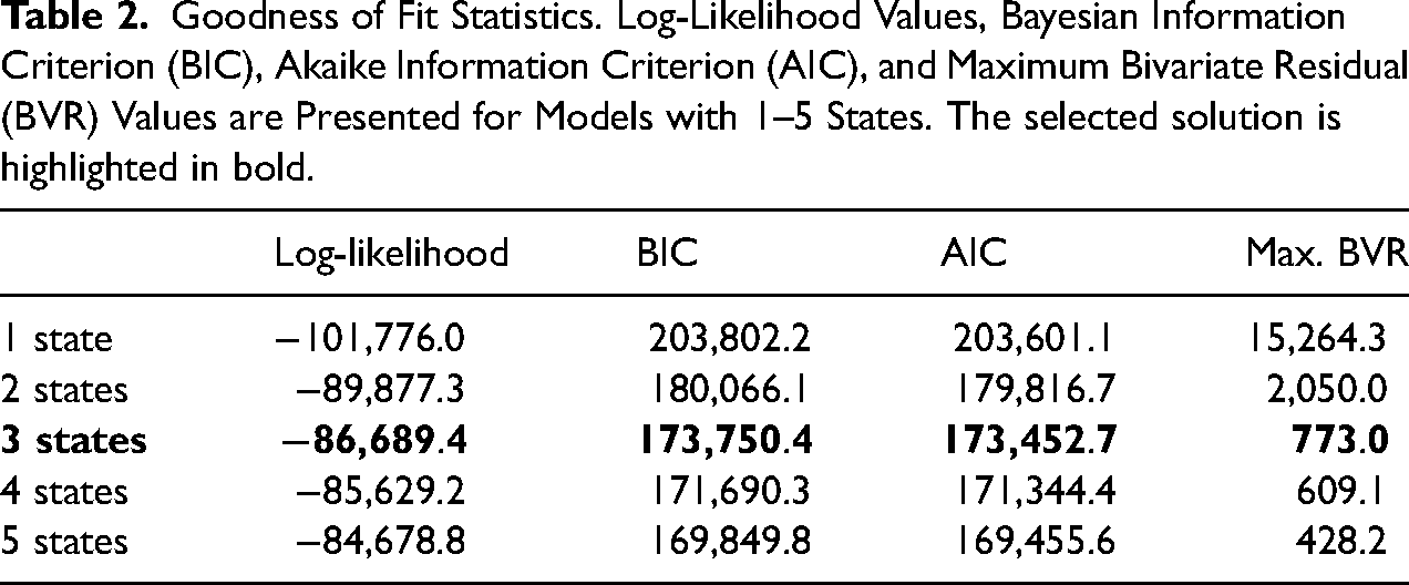
Table 3 shows the state membership probabilities for 2018–2021 under the hypothetical scenarios “always employed” and “never employed.” As can be seen, there are significant ATEs for the state membership probabilities in state 3 for all years. For example, for year 2018, the state membership probability in state 3 “poor mental health” under exposure “never employed” was 3.5 percentage points (confidence interval (CI) [0.2; 7.3]) higher than under exposure “always employed.” For all four years, the ATE was above 3 percentage points. Thus, not being employed throughout the study period results in at least a 3-percentage point higher probability of membership in the “poor mental health” state in comparison to being employed throughout the study period. ATEs for states 1 and 2 are not significant. Thus, being employed compared to not being employed throughout the study period did not increase the probability of membership in the “good mental health” state and the “slightly elevated mental health problems” state.

Table 3.

State^a Membership Probabilities and 95% CI at Each Year Under the Hypothetical Scenarios “Always Employed” and “Never Employed.”

		2018	2019	2020	2021
Always employed	State 1	0.500 [0.475; 0.527]	0.553 [0.528; 0.578]	0.455 [0.428; 0.479]	0.502 [0.476; 0.527]
	State 2	0.342 [0.322; 0.361]	0.304 [0.284; 0.326]	0.346 [0.327; 0.365]	0.331 [0.311; 0.350]
	State 3	0.159 [0.142; 0.177]	0.142 [0.126; 0.159]	0.199 [0.182; 0.216]	0.166 [0.148; 0.183]
Never employed	State 1	0.463 [0.418; 0.511]	0.524 [0.483; 0.567]	0.424 [0.380; 0.471]	0.473 [0.423; 0.527]
	State 2	0.343 [0.301; 0.384]	0.304 [0.268; 0.343]	0.340 [0.299; 0.381]	0.321 [0.273; 0.367]
	State 3	0.194 [0.165; 0.228]	0.172 [0.147; 0.200]	0.236 [0.205; 0.270]	0.206 [0.173; 0.243]
ATE	State 1	0.037 [−0.020; 0.087]	0.030 [−0.017; 0.073]	0.031 [−0.023; 0.079]	0.029 [−0.035; 0.086]
	State 2	−0.002 [−0.047; 0.045]	0.000 [−0.038; 0.035]	0.006 [−0.036; 0.053]	0.010 [−0.039; 0.064]
	State 3	−0.035 [−0.073; −0.002]	−0.030 [−0.059; −0.003]	−0.037 [−0.073; −0.002]	−0.039 [−0.080; 0.000]

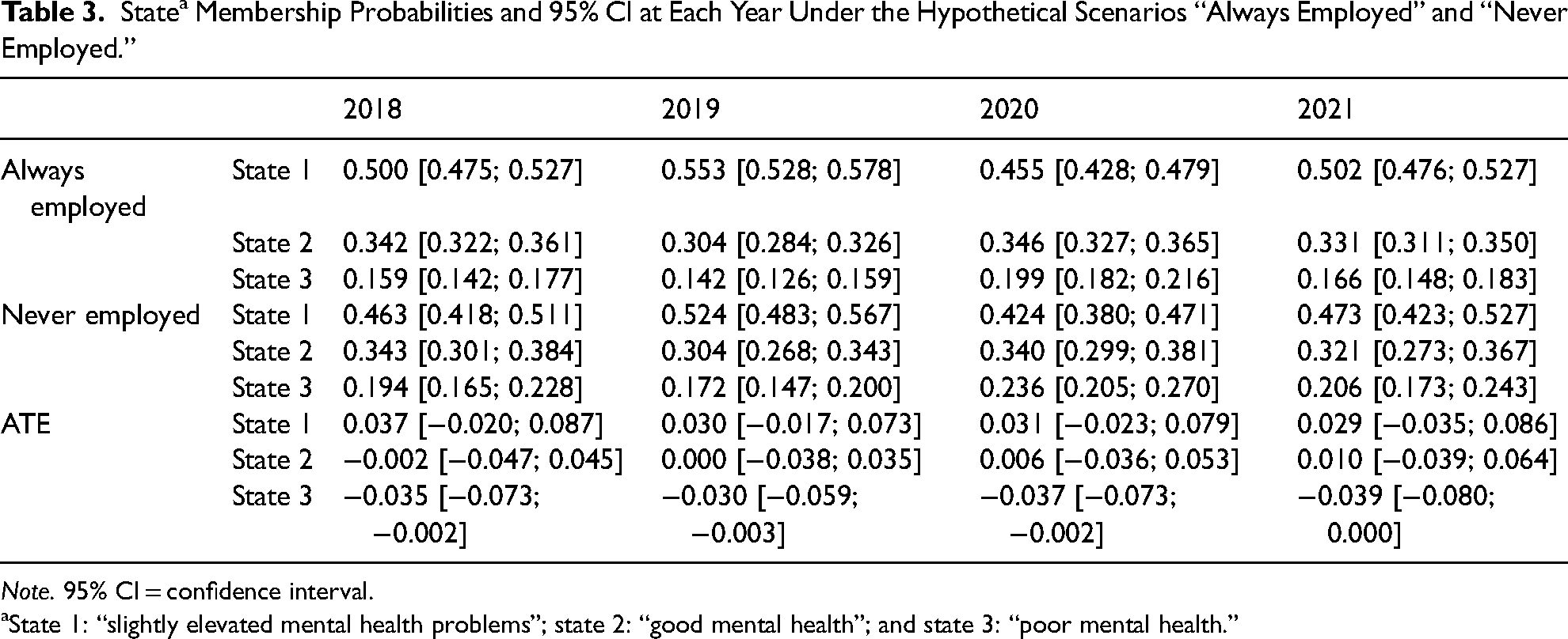
Note. 95% CI = confidence interval.

State 1: “slightly elevated mental health problems”; state 2: “good mental health”; and state 3: “poor mental health.”

Discussion

In this article, we present an analysis strategy for using LMMs in the g-formula to estimate causal effects when the outcome is not directly observed but measured through multiple indicators. Following the steps described above for implementing bias-adjusted three-step LMMs in the g-formula allows us to account for the intermediate confounding that arises when evaluating causal effects of time-varying exposures. To implement this strategy, we use three-step bias-adjusted LMMs which allows us to estimate a measurement model for the latent outcome that will be fixed in the consecutive steps. The latent states that are constructed in this first step are then used to estimate the structural models defining the relationships between confounders, exposure, and the outcome, that is, state membership. The g-formula can then be applied as usual, that is, the structural models of the LMM replace the generalized linear models that are otherwise commonly used in the g-formula. The consecutive simulation step in the g-formula is unaffected by the fact that our outcome is latent rather than directly observable. Notably, the use of three-step bias-adjusted LMMs is imperative for making this analysis strategy work. In the g-formula, several structural models need to be specified. Only when estimating the measurement model first and keeping it fixed for the consecutive steps, we can ensure that the latent states have the same definition in all models. That is, using one-step LMMs, the inclusion of covariates or multiple distal outcomes can alter the definition of the latent states resulting in essentially differently defined outcomes for all models used in the g-formula. Results from the simulation steps based on these models would then be meaningless. Furthermore, we expect the presented approach of using LMMs in the g-formula to perform better than alternative approaches using IPW as these methods typically produce larger standard errors. However, a comparison of these methods is beyond the scope of this paper and a topic for further research. As demonstrated in this study, our proposed method is very flexible, allowing for the rather straightforward implementation of extensions. For instance, one could consider a time-varying continuous latent outcome using a three-step structural equation modeling approach with an autoregressive model for the outcome.

A potential drawback of our newly proposed method is the g-null paradox. The g-null paradox states that if (1) the counterfactual mean as the ATE is identified by the parametric g-formula, (2) the time-varying confounders are affected by past exposure, and (3) the outcome at any time is not affected by exposure (sharp null hypothesis is true), then the g-formula cannot generally be correctly characterized by parametric models, unless these models are saturated (Robins and Wasserman 1997). Furthermore, McGrath, Young, and Hernan (2022) show that even if the exposure has a non-null causal effect, the g-formula estimate will be biased if the parametric models are specified too parsimoniously. The g-null paradox will similarly apply to our proposed method of using LMMs in the g-formula. However, null hypothesis significance testing is not usually a concern when using the g-formula because the primary interest lies in effect estimation. While the g-null paradox refers to a small source of bias, other sources such as confounding or measurement error are much more severe. Furthermore, the comparison of the natural course scenario and the empirical data in our exemplary data analysis revealed no substantial differences indicating that our structural models are not misspecified minimizing the risk of the g-null paradox being present.

Before implementing the g-formula, inferring causality requires clearly defining the estimand (Luijken et al. 2023). It is worth noting that this is not a trivial task, especially when using LMMs. First, one must decide on which state(s) to consider as the outcome of interest. For instance in our example, we investigated the difference in state membership probabilities between the two exposure groups for state 3 “poor mental health.” However, this definition of the estimand depends entirely on the results from the measurement model. Only after deciding on the number of latent states and defining the final measurement model, one can investigate which state might be of interest. As this step is exploratory by nature, no general recommendation can be given on how to define the estimand other than that this process should be informed by theory as much as possible. Second, one must decide on which contrast in the exposure to consider. The advantage of the g-formula is that it gives the researcher considerable freedom on which (hypothetical) scenarios to investigate. In this study, we investigated the ATE corresponding to the hypothetical scenarios “always employed” and “never employed.” That is, we created these scenarios within the g-formula by setting the exposure to always equal to one or always equal to zero in the simulation step. However, alternative definitions are possible. For instance, one might consider the ATT by comparing the natural course to the hypothetical scenario of “always employed.” This would be akin to approximating how a real-world intervention that reduces non-employment might affect mental health. Other hypothetical scenarios such as a constant changes of zeros and ones (“being in between jobs”) or job loss after a longer period of employment could be modeled although this might require some changes to the underlying models. While a clear definition of the estimand is imperative for inferring causality as has been highlighted before (Luijken et al. 2023), it seemingly does not always receive the required attention.

A potential issue to consider when using measurement models is measurement non-invariance (MNI) or differential item functioning. Meaningful comparisons between the groups, that is, exposed and unexposed individuals, are only possible if measurement invariance holds (D'Urso et al. 2022; Kankaraš and Moors 2014). However, this is often not the case in reality (Masyn 2017; Vermunt and Magidson 2021a). MNI is for instance violated when the relationship between the latent variable and some of the indicators is different for the two exposure groups or for individuals with specific values on some of the confounders. In our example, one could imagine that the item about happiness might be differently understood depending on the individual's origin. In such a case, these relationships need to be modeled by including direct effects between the corresponding covariates and indicators as has been shown by Vermunt and Magidson (2021a) and Clouth, Pauws, and Vermunt (2023). Although MNI can cause a large bias in the estimate of the ATE, testing for MNI seems to be an uncommon practice (D'Urso et al. 2022). However, how to proceed with including direct effects in the g-formula is unclear as these direct effects will alter the definition of the latent states and one might want to adjust for different sets of confounders in different structural models. In the interest of clarity, we did not consider MNI in this illustration and the problem remains a topic for future research.

Another challenge that needs to be addressed when implementing the g-formula in practice is missing data. Here, it is important to distinguish between two types of missing data, missing values on the indicators and missing values on the confounders and exposure. Missing values on the indicators are accounted for when constructing the measurement model. Assuming missingness at random, the estimation of the measurement model with missing data is straightforward using full-information maximum likelihood estimation (Dong and Peng 2013). Only if missing values on the indicators depend on values of the auxiliary variables, missingness becomes not at random when using the bias-adjusted three-step approach and estimates can be biased (Alagöz and Vermunt 2022). In this case, an alternative strategy for imputation is required. For missing values on the confounders and exposure, multiple imputation is required. As this article serves an educational purpose, we imputed a single set and considered the data complete for demonstrating the use of the g-formula. However, multiple imputation can be implemented in the g-formula. In fact, multiple imputation and the g-formula are closely related (Westreich et al. 2015). That is, Bartlett, Olarte Parra, and Daniel (2023) describe how to impute missing values based on the sequential models described in equation (4) and provide the R package gFormulaMI where this procedure is readily implemented.

Conclusion

In this article, we present an analysis strategy for using LMMs in the g-formula. The g-formula can be used for estimating causal effects in the presence of intermediate confounding. However, when the outcome is not directly observed but measured through multiple indicators, a measurement model is required. Here, we show how three-step bias-adjusted LMMs can be used for this, that is, by separately estimating the measurement model and implementing the g-formula using the structural models. Illustrating this approach, we estimated a small ATE of non-employment on the latent state “poor mental health” accounting for the temporal interrelation of employment status and mental health. Furthermore, the flexibility of the presented approach allows for a large variety of alternative definitions of the causal effect supporting a vast variety of practical applications.

Supplemental Material

sj-pdf-1-smr-10.1177_00491241251377068 - Supplemental material for Causal Inference for Latent Markov Models Using the Parametric G-Formula

Supplemental material, sj-pdf-1-smr-10.1177_00491241251377068 for Causal Inference for Latent Markov Models Using the Parametric G-Formula by Felix J. Clouth, Maarten J. Bijlsma, Steffen Pauws and Jeroen K. Vermunt in Sociological Methods & Research

Footnotes

Code Availability Statement

The code used during this study and documentation for the code are available on the Clouth 2025 (GitHub repository): “Causal-inference-for-latent-Markov-models-using-the-parametric-G-formula,” .

Data Availability Statement

The data were used under license from LISS Data Archive for the current study and are not publicly available. However, the data can be accessed following the instructions provided in the R script accompanying this manuscript.

Declaration of Conflicting Interests

The authors declared the following potential conflicts of interest with respect to the research, authorship, and/or publication of this article: Jeroen K. Vermunt is a co-developer (along with Jay Magidson) of LatentGOLD software. While LatentGOLD is a commercial program, as of January 2025, it is free for academic use. The remaining authors declared no potential conflicts of interest.

Funding

The authors disclosed receipt of the following financial support for the research, authorship, and/or publication of this article: This work was supported by The Netherlands Organisation for Scientific Research (NWO) (grant number 628.001.030).

Preregistration Statement

This study was not preregistered as it used publicly available data that already existed before the study was begun.

ORCID iDs

Felix J. Clouth

Steffen Pauws

Supplemental Material

Supplemental material for this article is available .

Notes

Author Biographies

Dr. Felix J. Clouth is an assistant professor at the Department of Methodology and Statistics at Tilburg University and visiting researcher at the Department of Population, Policy & Practice at the University College London. His research deals with the integration of latent variable models with modern causal inference methods and the transportability of causal effects utilizing sampling weights.

Dr. Maarten J. Bijlsma is a clinical data scientist at the Netherlands Comprehensive Cancer Organisation and affiliated with the Groningen Research Institute of Pharmacy, University of Groningen and the Max Planck Institute for Demographic Research. His research interests are on the use of modern causal inference methods on large-scale registry-based data sets.

Prof. Dr. Steffen Pauws is a professor at the Department of Communication and Cognition at Tilburg University. His research interests are on risk modeling and communication in healthcare as well as the implementation of risk models in patient pathways.

Prof. Dr. Jeroen K. Vermunt is a professor at the Department of Methodology and Statistics at Tilburg University. His research interests are on the methodology of social, behavioral, and biomedical research, with a special focus on latent variable models and techniques for the analysis of categorical, multilevel, and longitudinal data sets. He is a co-developer (along with Jay Magidson) of LatentGOLD software.

References

Alagöz

Ö. E. C

Vermunt

J. K.

. 2022. “Stepwise Latent Class Analysis in the Presence of Missing Values on the Class Indicators.” Structural Equation Modeling: A Multidisciplinary Journal 29(5):784–90.

Bakk

Tekle

F. B.

Vermunt

J. K.

. 2013. “Estimating the Association Between Latent Class Membership and External Variables Using Bias-Adjusted Three-Step Approaches.” Sociological Methodology 43(1):272–311. 10.1177/0081175012470644

Bartlett

J. W.

Olarte Parra

Daniel

R. M.

. 2023. “G-formula for Causal Inference via Multiple Imputation.” arXiv.

Bartolucci

Farcomeni

Pennoni

. 2013. Latent Markov Models for Longitudinal Data. Chapman & Hall/CRC. Boca Raton, FL.

Bartolucci

Montanari

Pandolfi

. 2015. “Three-Step Estimation of Latent Markov Models with Covariates.” Computational Statistics and Data Analysis 83:287–301.

Bartolucci

Pennoni

Vittadini

. 2016. “Causal Latent Markov Model for the Comparison of Multiple Treatments in Observational Longitudinal Studies.” Journal of Educational and Behavioral Statistics 41(2):146–79. 10.3102/1076998615622234

Bartolucci

Pennoni

Vittadini

. 2023. “A Causal Latent Transition Model with Multivariate Outcomes and Unobserved Heterogeneity: Application to Human Capital Development.” Journal of Educational and Behavioral Statistics 48(4):387–419. 10.3102/10769986221150033

Bavaro

Tullio

. 2024. “A Cycle or a Tunnel? A Study on Unemployment and Low-Pay Dynamics in Italy.” Labour Economics 90.

Bijlsma

M. J.

Tarkiainen

Myrskyla

Martikainen

. 2017. “Unemployment and Subsequent Depression: A Mediation Analysis Using the Parametric G-Formula.” Social Science & Medicine 194:142–50. 10.1016/j.socscimed.2017.10.011

10.

Bijlsma

M. J.

Wilson

Tarkiainen

Myrskyla

Martikainen

. 2019. “The Impact of Unemployment on Antidepressant Purchasing: Adjusting for Unobserved Time-Constant Confounding in the G-Formula.” Epidemiology 30(3):388–95. 10.1097/EDE.0000000000000985

11.

Bolck, A., M. Croon, and J. Hagenaars. 2004. “Estimating Latent Structure Models with Categorical Variables: One-Step Versus Three-Step Estimators.” Political Analysis 12(1):3-27.

12.

Bollen

K. A.

2002. “Latent Variables in Psychology and the Social Sciences.” Annual Review of Psychology 53:605–34.

13.

Bray

B. C.

Dziak

J. J.

Patrick

M. E.

Lanza

S. T.

. 2019. “Inverse Propensity Score Weighting with a Latent Class Exposure: Estimating the Causal Effect of Reported Reasons for Alcohol Use on Problem Alcohol Use 16 Years Later.” Prevention Science 20(3):394–406. 10.1007/s11121-018-0883-8

14.

Bubonya

Cobb-Clark

D. A.

Ribar

D. C.

. 2019. “The Reciprocal Relationship Between Depressive Symptoms and Employment Status.” Economics & Human Biology 35:96–106. 10.1016/j.ehb.2019.05.002

15.

Clouth . 2025. felixclouth/Causal-inference-for-latent-Markov-models-using-the-parametric-G-formula: New Release (new_release). Zenodo. https://doi.org/10.5281/zenodo.16569766

16.

Clouth

F. J.

Pauws

Mols

Vermunt

J. K.

. 2022. “A New Three-Step Method for Using Inverse Propensity Weighting with Latent Class Analysis.” Advances in Data Analysis and Classification 16(2):351–71. 10.1007/s11634-021-00456-5

17.

Clouth

F. J.

Pauws

Vermunt

J. K.

. 2023. “Three-Step Latent Class Analysis with Inverse Propensity Weighting in the Presence of Differential Item Functioning.” Structural Equation Modeling: A Multidisciplinary Journal 30(5):737–48. 10.1080/10705511.2022.2161384

18.

Cole

S. R.

Frangakis

C. E.

. 2009. “The Consistency Statement in Causal Inference: A Definition or an Assumption?” Epidemiology 20(1):3–5. 10.1097/EDE.0b013e31818ef366

19.

Collins

L. M.

Lanza

S. T.

. 2010. Latent Class and Latent Transition Analysis: With Applications in the Social, Behavioral, and Health Sciences. Hoboken. NJ: Wiley.

20.

Daniel

R. M.

Cousens

S. N.

De Stavola

B. L.

Kenward

M. G.

Sterne

J. A.

. 2013. “Methods for Dealing with Time-Dependent Confounding.” Statistics in Medicine 32(9):1584–618. 10.1002/sim.5686

21.

Di Mari

Oberski

D. L.

Vermunt

J. K.

. 2016. “Bias-Adjusted Three-Step Latent Markov Modeling with Covariates.” Structural Equation Modeling: A Multidisciplinary Journal 23(5):649–60. 10.1080/10705511.2016.1191015

22.

Dong

Peng

C. Y. J.

. 2013. “Principled Missing Data Methods for Researchers.” SpringerPlus 2:222. 10.1186/2193-1801-2-222

23.

D'Urso

E. D.

Maassen

Van Assen

M. A. L. M.

Nuijten

M. B.

De Roover

Wicherts

J. M.

. 2022. “The Dire Disregard of Measurement Invariance Testing in Psychological Science.” PsyArXiv. https://osf.io/j72t4/?view_only=83cf802a792543419841d36cc885c702.

24.

Fish

G. A.

Leite

W. L.

. 2024. “Unreliable Continuous Treatment Indicators in Propensity Score Analysis.” Multivariate Behavioral Research 59(2):187–205. 10.1080/00273171.2023.2235697

25.

Frijters

Johnston

D. W.

Shields

M. A.

. 2014. “The Effect of Mental Health on Employment: Evidence from Australian Panel Data.” Health Economics 23(9):1058–71. 10.1002/hec.3083

26.

Goodman

L. A.

1974. “Exploratory Latent Structure Analysis Using Both Identifiable and Unidentifiable Models.” Biometrika 61(2):215–31. 10.1093/biomet/61.2.215

27.

X. S.

Rosenbaum

P. R.

. 1993. “Comparison of Multivariate Matching Methods: Structures, Distances, and Algorithms.” Journal of Computational and Graphical Statistics 2:405–20.

28.

Hernán

M. A.

Robins

J. M.

. 2006. “Estimating Causal Effects from Epidemiological Data.” Journal of Epidemiology and Community Health 60:578–86. 10.1136/jech.2004.029496

29.

Imai

Keele

Tingley

. 2010. “A General Approach to Causal Mediation Analysis.” Psychological Methods 15(4):309–34. 10.1037/a0020761

30.

Imbens

G. W.

2000. “The Role of the Propensity Score in Estimating Dose–Response Functions.” Biometrika 87(3):706–10.

31.

Imbens

G. W.

Wooldridge

J. M.

. 2009. “Recent Developments in the Econometrics of Program Evaluation.” Journal of Economic Literature 47(1):5–86. 10.1257/jel.47.1.5

32.

Jefferis

B. J.

Nazareth

Marston

Moreno-Kustner

Bellon

J. A.

Svab

Rotar

Geerlings

M. I.

Xavier

Goncalves-Pereira

Vicente

Saldivia

Aluoja

Kalda

King

. 2011. “Associations Between Unemployment and Major Depressive Disorder: Evidence from an International, Prospective Study (the Predict Cohort).” Social Science & Medicine 73(11):1627–34. 10.1016/j.socscimed.2011.09.029

33.

Kankaraš

Moors

. 2014. “Analysis of Cross-Cultural Comparability of PISA 2009 Scores.” Journal of Cross-Cultural Psychology 45(3):381–99. 10.1177/0022022113511297

34.

Keil

A. P.

Edwards

J. K.

Richardson

D. B.

Naimi

A. I.

Cole

S. R.

. 2014. “The Parametric G-Formula for Time-to-Event Data: Intuition and a Worked Example.” Epidemiology 25(6):889–97. 10.1097/EDE.0000000000000160

35.

King

Tomz

Wittenberg

. 2000. “Making the Most of Statistical Analyses: Improving Interpretation and Presentation.” American Journal of Political Science 44(2):341–55.

36.

Lanza

S. T.

Coffman

D. L.

. 2013. “Causal Inference in Latent Class Analysis.” Structural Equation Modeling: A Multidisciplinary Journal 20(3):361–83. 10.1080/10705511.2013.797816

37.

Layard

2013. “Mental Health: The New Frontier for Labour Economics.” IZA Journal of Labor Policy 2. 10.1186/2193-9004-2-2

38.

Lazarsfeld

P. F.

Henry

N. W.

. 1968. Latent structure analysis. Houghton Mill. Boston, MA.

39.

Lepine

J. P.

Briley

. 2011. “The Increasing Burden of Depression.” Neuropsychiatric Disease and Treatment 7(Suppl 1):3–7. 10.2147/NDT.S19617

40.

Luijken

van Eekelen

Gardarsdottir

Groenwold

R. H. H.

van Geloven

. 2023. “Tell Me What You Want, What You Really Really Want: Estimands in Observational Pharmacoepidemiologic Comparative Effectiveness and Safety Studies.” Pharmacoepidemiology and Drug Safety 32(8):863–72. 10.1002/pds.5620

41.

Masyn

K. E.

2017. “Measurement Invariance and Differential Item Functioning in Latent Class Analysis with Stepwise Multiple Indicator Multiple Cause Modeling.” Structural Equation Modeling: A Multidisciplinary Journal 24(2):180–97. 10.1080/10705511.2016.1254049

42.

McGrath

Young

J. G.

Hernan

M. A.

. 2022. “Revisiting the G-Null Paradox.” Epidemiology 33(1):114–20. 10.1097/EDE.0000000000001431

43.

Naimi

A. I.

Cole

S. R.

Kennedy

E. H.

. 2017. “An Introduction to G Methods.” International Journal of Epidemiology 46(2):756–62. 10.1093/ije/dyw323

44.

Olesen

S. C.

Butterworth

Leach

L. S.

Kelaher

Pirkis

. 2013. “Mental Health Affects Future Employment as Job Loss Affects Mental Health: Findings from a Longitudinal Population Study.” BMC Psychiatry 13(144).

45.

Pennoni

Paas

Bartolucci

. 2023. “A Causal Hidden Markov Model for Assessing Effects of Multiple Direct Mail Campaigns.” TEST 32:1336–64.

46.

Robins

1986. “A New Approach to Causal Inference in Mortality Studies with a Sustained Exposure Period - Application to Control of the Healthy Worker Survivor Effect.” Mathematical Modelling 7(9-12):1393–512.

47.

Robins

Wasserman

. 1997. “Estimation of Effects of Sequential Treatments by Reparameterizing Directed Acyclic Graphs.” Proceedings of the Thirteenth Conference on Uncertainty in Artificial Intelligence. Morgan Kaufmann Publishers Inc.

48.

Rosenbaum

P. R.

Rubin

D. B.

. 1983. “The Central Role of the Propensity Score in Observational Studies for Causal Effects.” Biometrika 70:41–55.

49.

Rudolph

J. E.

Cartus

Bodnar

L. M.

Schisterman

E. F.

Naimi

A. I.

. 2022. “The Role of the Natural Course in Causal Analysis.” American Journal of Epidemiology 191(2):341–8. 10.1093/aje/kwab248

50.

Steele

French

Bartley

. 2013. “Adjusting for Selection Bias in Longitudinal Analyses Using Simultaneous Equations Modeling. The Relationship Between Employment Transitions and Mental Health.” Epidemiology 24(5):703–11.

51.

Tullio

Bartolucci

. 2022. “Causal Inference for Time-Varying Treatments in Latent Markov Models: An Application to the Effects of Remittances on Poverty Dynamics.” Annals of Applied Statistics 16(3):1962–85. 10.1214/21-AOAS1578

52.

Van Buuren

Groothuis-Oudshoorn

. 2011. “mice: Multivariate Imputation by Chained Equations in R.” Journal of Statistical Software 45(3):1–67. http://www.jstatsoft.org/ .

53.

VanderWeele

T. J.

2022. “Constructed Measures and Causal Inference: Towards a New Model of Measurement for Psychosocial Constructs.” Epidemiology 33(1):141–51. 10.1097/EDE.0000000000001434

54.

Vermunt

J. K.

2010. “Latent Class Modeling with Covariates: Two Improved Three-Step Approaches.” Political Analysis 18:450–69.

55.

Vermunt

J. K.

Langeheine

Bockenholt

. 1999. “Discrete-Time Discrete-State Latent Markov Models with Time-Constant and Time-Varying Covariates.” Journal of Educational and Behavioral Statistics 24(2):179–207.

56.

Vermunt

J. K.

Magidson

. 2021a. “How to Perform Three-Step Latent Class Analysis in the Presence of Measurement Non-Invariance or Differential Item Functioning.” Structural Equation Modeling: A Multidisciplinary Journal 28(3):356–64.

57.

Vermunt

J. K.

Magidson

. 2021b. LG-Syntax User's Guide: Manual for Latent GOLD Syntax Module Version 6.0. http://www.statisticalinnovations.com.

58.

Ware

J. E.

Snow

K. K.

Kosinski

Gandek

. 2000. SF-36 Health Survey: Manual and Interpretation Guide. QualityMetric Inc. Lincoln. NE.

59.

Westreich

Edwards

J. K.

Cole

S. R.

Platt

R. W.

Mumford

S. L.

Schisterman

E. F.

. 2015. “Imputation Approaches for Potential Outcomes in Causal Inference.” International Journal of Epidemiology 44(5):1731–7. 10.1093/ije/dyv135

60.

Wiggins

1955. “Mathematical Models for the Analysis of Multi-Wave Panels.” PhD Dissertation, Columbia University.

Supplementary Material

Please find the following supplemental material available below.

For Open Access articles published under a Creative Commons License, all supplemental material carries the same license as the article it is associated with.

For non-Open Access articles published, all supplemental material carries a non-exclusive license, and permission requests for re-use of supplemental material or any part of supplemental material shall be sent directly to the copyright owner as specified in the copyright notice associated with the article.

0.00 MB

0.32 MB