
Abstract
Models for time-to-event data are based on transition rates between states, and to define such hazards of experiencing an event, the time scale over which the process evolves needs to be identified. In many applications, however, more than one time scale might be of importance. Here, we demonstrate how to model a hazard jointly over two time dimensions. The model assumes a smooth bivariate hazard function, and the function is estimated by two-dimensional
Introduction
Analysis of time-to-event data focuses on the timing of successive transitions between states of interest and the effect of covariates on the occurrence of these transitions. The life course can be viewed as a sequence of such transitions or events, and a common statistical framework to analyze how life courses evolve is a stochastic process with a continuous time scale and a finite number of states (Blossfeld et al. 1989), that is, a multi-state model. In its most reduced form, the former simplifies to survival analysis. Only one event is considered: the process starts at birth and is ended by the event “death” and the time scale is the age of the individual. When modeling transitions from one state to another in the life course, hazard models are the most common approach. Hazard functions capture the time-dependent instantaneous risk of an event, given the transition has not yet occurred, and by definition depend on the time scale of the process.
Time is, therefore, key in understanding any event history analysis, and each time scale is defined with respect to a reference event, for example, birth (Hobcraft and Murphy 1986). In demographic analyses, the most prominent time scale is age, which is time since birth. This is because many of the life transitions, such as leaving parental home, completing education, entering a first union or birth of the first child, are thought to be age-dependent. Demographers refer to statistical regularities in the timing of demographic events in a population as “age norm” (Settersten 2003). Consequently, age-specific transition rates are the most frequent choice.
But different time scales can be relevant when analyzing the occurrence of an event like, for example, marriage or divorce. It has long been argued that other time dimensions, such as the duration since entry into the current state, are also of interest (Hobcraft and Murphy 1986). For example, if the timing of the first child birth within a marital union is of interest, the hazard of first birth strongly depends on the age of the mother, as women’s fertility declines with increasing age. However, the duration of the marriage is of equal importance, as couples might base the decision of having a child on the time elapsed since their marriage. The duration of the marriage, therefore, represents another time scale over which the hazard of marital child birth changes.
Standard hazard models require the choice of one time scale over which the risk of observing an event evolves (Klein and Moeschberger 2005). This choice is usually based on previous knowledge of the phenomenon under study. While in demography, age-specific rates are commonly preferred, in medical and epidemiological studies, when disease progression is analyzed, time since diagnosis or disease onset might be the first choice. If additional time scales are present and acknowledged, a common strategy is to incorporate the second time dimension as a categorized fixed or time-varying covariate in the model. Alternatively, a more flexible approach often used to deal with non-proportionality of the hazards is to account for time-varying effects of a fixed covariate, for example, by estimating a time-varying effect of the age at entry into the risk set (Bender et al. 2018).
In demography, there have been attempts to model the hazard of an event directly as a function of more than one time dimension. An early attempt to model the hazard of marital childbearing by age and duration of marriage comes from Page (1977), who models fertility rates as a function of age, cohort, and marriage duration. The Page model is rather inflexible in the way the hazard depends on these time scales, and it requires a parametric formulation of the effect of each time scale on the hazard. Other examples of models that consider hazard functions simultaneously over two time axes can be found in the medical statistical literature (Batyrbekova et al. 2022; Bower et al. 2022; Efron 2002; Iacobelli and Carstensen 2013; Rebora et al. 2015), but the issue has rarely been explored in the social sciences.
With this paper, we aim to shed light on the overlooked aspect of multiple time scales in event history analysis within a field of application where it has not received thorough examination. We review some approaches to model hazards over two time scales simultaneously, which differ in how flexibly the effect of the second time scale is modeled. The models make only modest assumptions about the bivariate hazard, namely that the function evolves smoothly over both time domains. We estimate the models by
To illustrate the approach, we study transitions from unmarried cohabitation to marriage or to separation by age of the individual and duration of the cohabitation. Age certainly has a major role in determining the transitions from cohabitation to a subsequent state; however, previous research has favored duration of the cohabitation as the main time scale for such transitions (Di Giulio et al. 2019; Hiekel et al. 2015). We argue that the two time dimensions will likely interact with each other and that the hazard of marrying or separating is determined simultaneously by both time scales. We explore these questions using data from the German Family Panel (pairfam) (Brüderl et al. 2020a).
This study contributes to the literature on modeling time-to-event socio-demographic data in several ways. First, we provide theoretical and practical reasoning to consider more than one time scale for the analysis of time-to-event data, with a particular focus on demographic processes. Second, we review the
In Section “Temporal Change: Time Scales, Covariates, Effects,” we first discuss time scales in event history analysis and how additional time scales can enter as covariates in the model. Then, we describe the two-dimensional
Temporal Change: Time Scales, Covariates, Effects
Social sciences are concerned, among other things, with the study of temporal change. On the individual level, change often is marked by the occurrence of events, such as obtaining an educational degree, moving out of parental home, marriage, birth of a child, divorce, entering retirement, and ultimately death—just to name a few out of a long list. The technical vehicle to study such histories of events is stochastic processes, that is, random variables indexed by time that describe the occurrence of the event of interest probabilistically.
The time scale over which the process is modeled commonly is obvious—the age of the individual or time since marriage—but temporal change often occurs along several time scales simultaneously. Individuals change their attitudes and behavior with age, but also macro environment changes with calendar time, which influence the occurrence of the event of interest. The concept of individual life courses evolving along several time scales is long known, and portraying processes along two time scales is familiar to social scientists ever since Lexis (1875). If more than one time scale is relevant, then all should enter the analysis, and their importance should be assessed properly.
When the occurrence of events is studied, then hazard-based models are the most common choice. For a single time scale
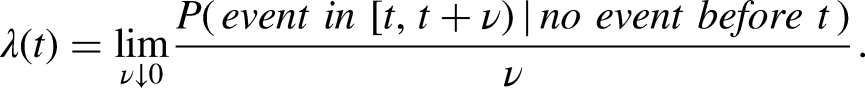
Time scales differ only in their origin, and they move at the same speed, so that an increment of one time unit on one scale corresponds to the same increment on the other scale. Because of the same speed, when portrayed in a so-called Lexis diagram, individuals move along a diagonal line with slope 1 (Keiding 1990) (see Figure 1(a)). In the application presented in Section “Transitions From Cohabitation to Marriage or Separation,” we will study transitions out of unmarried cohabitation (separation or marriage) and the two time scales will be age (denoted by
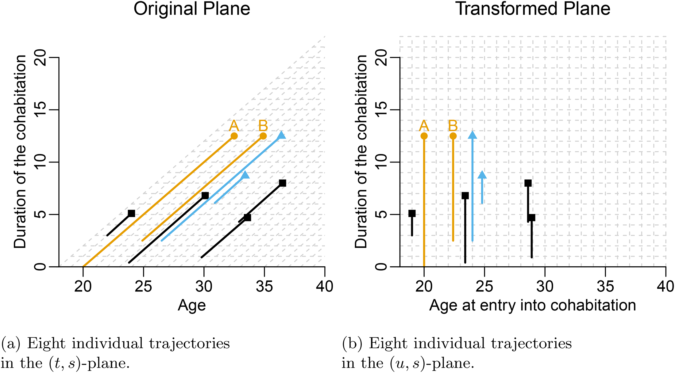
Eight individual trajectories for cohabitation until marriage, separation, or censoring. The panel on the left shows the trajectories in the
The two time scales hazard

and it is the instantaneous risk of experiencing an event at age
In the example, time scale
The point in time
In the cohabitation example, employing

where
The elaboration above demonstrates that for estimating a hazard along two time scales,
In the simplest case, when only one time scale matters, then
Models for
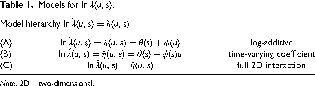
Note. 2D = two-dimensional.
In Model (A), the same baseline shape
For estimating Models (A) to (C), we will employ univariate or bivariate
Alternative approaches to model and estimate hazards as functions over two time dimensions have been described in the literature. The two-way model proposed by Efron (2002) expresses the log-hazard as the sum of two baseline hazards, polynomials in this case, each estimated over one of the two time scales. More versatile versions of this model include flexible parametric functions of the two time scales (Batyrbekova et al. 2022; Bower et al. 2022; Iacobelli and Carstensen 2013). A full interaction model, although in principle possible, to our knowledge has not been implemented yet. Log-additive and varying-coefficient specifications have also been proposed in Bender et al. (2018), see also Bender and Scheipl (2018).
Smoothing Bivariate Hazard Rates With P-splines
Smoothing a univariate (single time scale) hazard
Bin-specific hazard levels
The concepts of univariate hazard smoothing with
The basic ingredients stay the same: the data, now extending over two time axes, are binned into bins of equal size (now squares or rectangles), and the log-hazard, which is a bivariate surface, is represented via linear combinations of
First, the two axes
The values
The log-likelihood is equivalent to that of a Poisson model for the counts 
The log-additive model (A) and the varying-coefficient model (B), see Section “Temporal Change: Time Scales, Covariates, Effects,” are straightforward extensions of the univariate
The log-additive model (A)
requires two smooth but univariate components. The functions 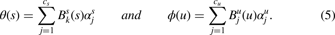
The rows of
With this particular structure, we can solve the system of equations obtained from maximizing the penalized log-likelihood of the model (as derived in Appendix equation (A.9), online supplement), this time depending on two smoothing parameters
For the varying coefficient model (B)
The most flexible model (C) is a smooth bivariate surface
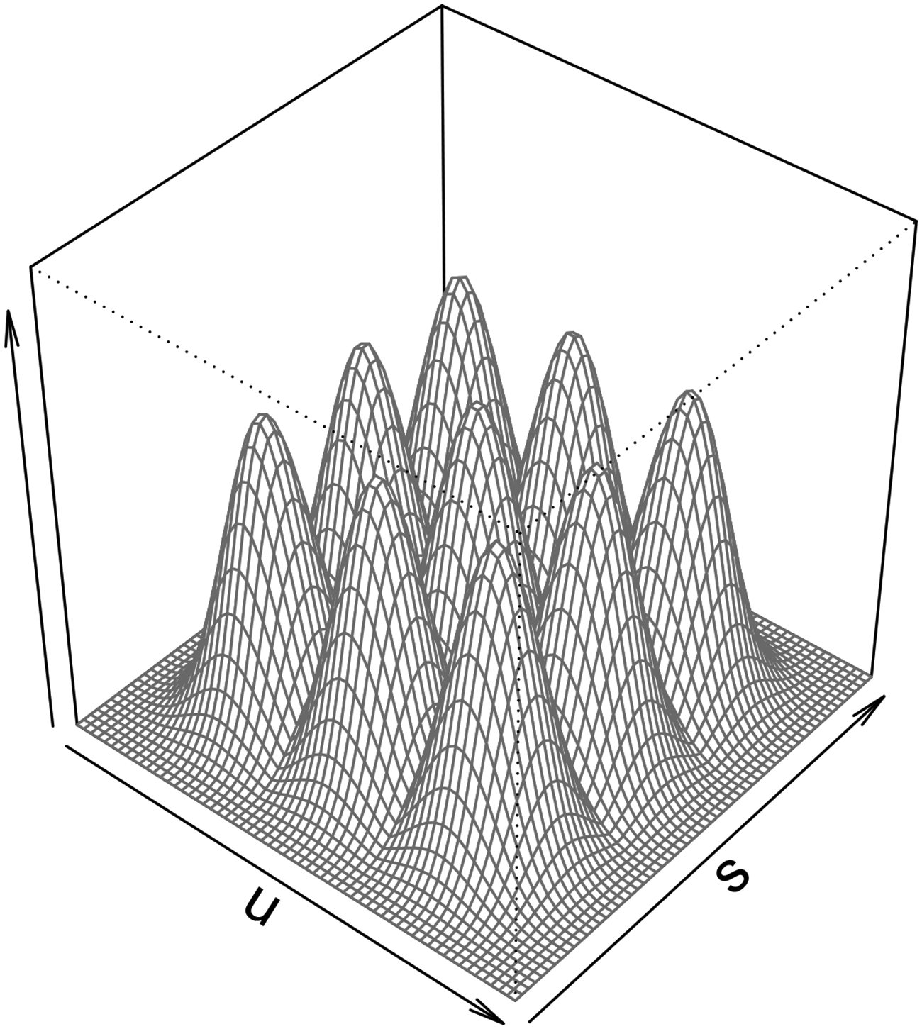
An example of a
More specifically, the model is as follows. Two marginal
Their tensor product
is of dimension
In this way, the model for the log-hazard becomes
While the extension to two dimensions is relatively straightforward, the notation can become cumbersome, and a clever arrangement of quantities will allow efficient computations. The 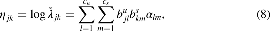
which in matrix notation simply is
In two dimensions, a penalty on the coefficients in 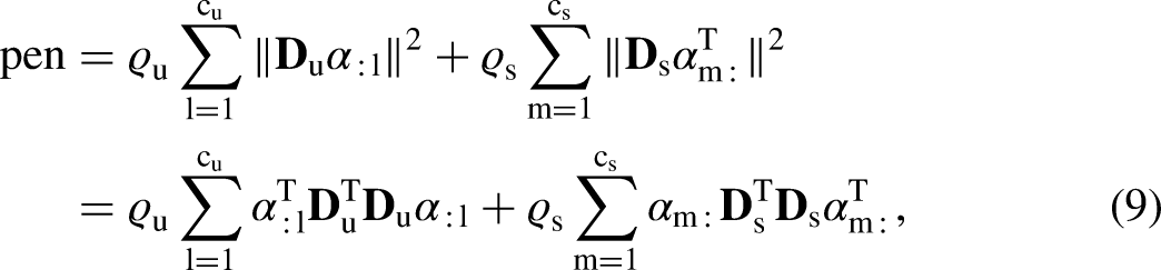
where the first term in the sum penalizes the columns of
The optimal values of the smoothing parameters are found by minimizing the Akaike information criterion (AIC) (or the Bayesian information criterion (BIC)), as a function of the pair (
Uncertainty estimates are derived as byproducts of the iterative weighted least square algorithm. The variance–covariance matrix of 
where
Transitions From Cohabitation to Marriage or Separation
Background
Premarital cohabitation, that is, living together with a romantic partner without being married, is a common form of living arrangement. In many countries in Europe and in the United States, premarital cohabitation has replaced direct marriage in the process of union formation (Sassler and Lichter 2020; Sobotka and Berghammer 2021). Therefore, scholars are increasingly interested in understanding the timing and determinants of transitions out of unmarried cohabiting unions. The majority of cohabiting individuals will eventually marry their partner (Nazio and Blossfeld 2003; Sassler and Lichter 2020), while some will experience the dissolution of their cohabitation (Hiekel et al. 2014). In order to provide a comprehensive picture of these processes, researchers need to properly account for two time scales, which are drivers of such transitions: duration of the cohabitation and age of the individual. However, published studies account for the presence of these two time scales only partly.
Research focused on the transitions out of cohabitation, either into marriage or into union dissolution, usually considers union duration as the most important time scale (Lu et al. 2012), while controlling for age at union formation (Hiekel et al. 2015; Wright 2019) or both age and age at start of cohabitation (Le 2002). Union duration is often considered as the main time scale for several reasons. Unmarried cohabitation can be seen as a trial marriage, in which individuals test the suitability of the partner as a spouse (Klijzing 1992). Since cohabiting couples learn about their compatibility over time, longer cohabitations might increase the risk of transitioning to marriage (Schnor 2014), while the risk of separation is higher at shorter durations. The latter is especially true for people who have started a cohabitation at a younger age, and therefore might be more likely to be in a poor match (Ermisch and Francesconi 2000).
Chronological age might be a proxy for internalized or ascribed norms for behaviors regarding life transitions (Settersten and Mayer 1997). Individuals often organize their lives around chronological age-deadlines (Settersten and Hagestad 1996). As an example, in a social context where childbearing is more widely accepted inside a marriage, such as in Western Germany, individuals might feel pressured to marry before they reach a certain age, to then transition to parenthood. Additionally, younger couples might be less likely to transition to marriage and more likely to undergo a union dissolution (Ermisch and Francesconi 2000). Hence, many authors study life transitions using chronological age as the time scale.
Following these theoretical considerations, we argue that both age and union duration are important time scales that influence the individuals’ decision to marry or to dissolve their cohabitation. Moreover, the hazard of these life events might be quite different for different combinations of age and duration of the cohabitation, indicating possibly complex interactions between the two time dimensions. For example, individuals who enter a cohabitation with their partner at a younger age might be less inclined to marry within a couple of years and therefore remain in unmarried cohabitation for longer times. Contrary to this, individuals and especially women, who start cohabiting in their thirties, might feel more (biological or societal) pressure to marry their partner quickly to successively transition to childbearing.
In the following, we show how models (A) to (C) described in Section “Temporal Change: Time Scales, Covariates, Effects” capture the interplay of age and duration in the hazard of ending an unmarried cohabitation, in either marriage or separation, and which level of complexity provides the best fit.
Data and Study Design
We use data from waves 1 to 11 of the pairfam (Panel Analysis of Intimate Relationships and Family Dynamics), release 11.0 (Brüderl et al. 2020a). A detailed description of the study can be found in Huinink et al. (2011).
Pairfam is a longitudinal panel survey, conducted annually, providing rich data on the formation and development of intimate relationships and families. The panel started with about 12,000 randomly selected individuals (anchors) of three different birth cohorts (1991–1993, 1981–1983, and 1971–1973) living in West and East Germany. The first wave of interviews was conducted in 2008. In 2009, about 1,500 individuals living in East Germany were sampled as part of the panel study DemoDiff, which was initiated following the design of pairfam. Beginning with wave five, the two studies have been fully integrated under pairfam. Finally, in 2019 (wave 11), a refreshment sample was drawn, which added new individuals from cohorts 1981–1983 and 1991–1993 together with a new cohort of individuals born in 2001–2003.
In this study, we use the dataset biopart, which is a ready-to-use dataset prepared by the pairfam team. The dataset biopart provides both retrospective and prospective information on individuals’ relationship histories from age 14, including cohabitations and marriages, on a monthly basis, and it is constructed with data collected in each wave. Details of biopart, as well as of the study design, can be found in the Data Manual (Brüderl et al. 2020b).
For this analysis, we included men and women living in East or West Germany who had experienced at least one non-marital cohabitation with a romantic partner of the opposite sex during the study period. At their first interview, individuals are asked to list all romantic relationships from age 14, together with the dates of important events (beginning of cohabitation, marriage, union dissolution, etc.). Therefore, information on all cohabiting unions before and after the first interview is available in the biopart dataset.
In our analysis, we include two sets of cohabitations: First, we include all unmarried cohabiting unions that were formed before but have not ended by the time of the first interview. For these cohabiting unions, the date of the first interview is taken as entry into the study. The cohabitation has been running at that point for a duration
These choices are visualized in Figure 3: here we represent all transitions between states that might be observed thanks to the design of pairfam and the data available in the biopart dataset.
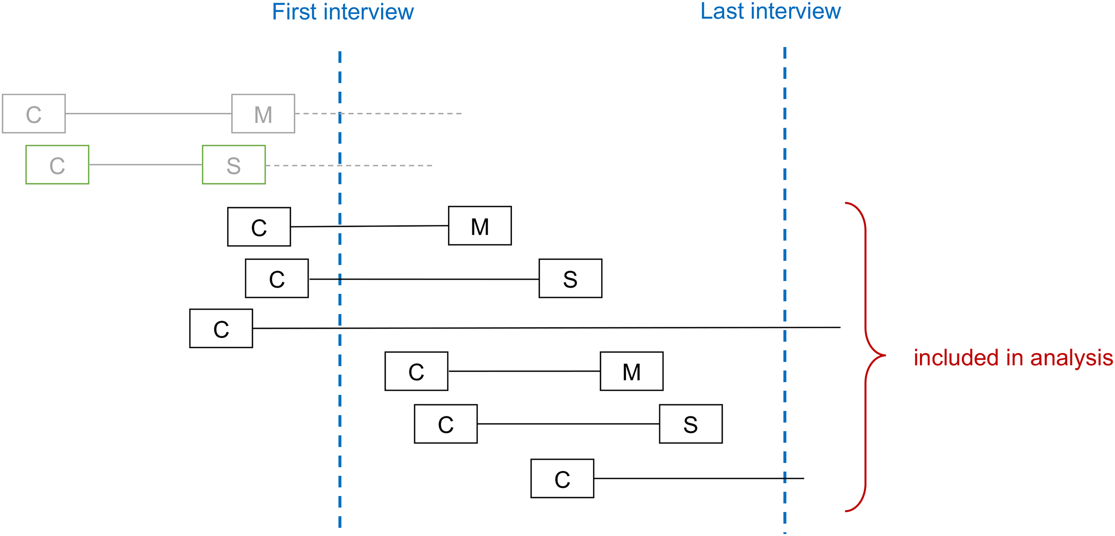
Sketch of biopart trajectories that were included in the analyses. C = Start of cohabitation, M = Marriage, S = Separation. Cohabiting unions that ended before the first interview were excluded. Cohabitations that started before the first interview were included and delayed entry (left truncation) was accounted for. Cohabitations that started during the observation period were also included in the analysis.
In the biopart dataset, there are 14,235 cohabitations, of which 8,451 had already ended before the first interview. Same-sex couples were excluded because regulations regarding same-sex marriages have changed during the study period (172 cohabitation). Additionally, we excluded 58 cohabitations that ended because of the partner’s death and 62 cohabitations with unclear ending dates. We also excluded cohabitations that started directly with a marriage (143 cohabitations). Finally, we only considered cohabitations that started when the individual was 18 years or older, which defines full legal age in Germany. Because of this age restriction, only one individual from the youngest cohort (2001–2003) would have entered our sample, so we decided to restrict to the three oldest cohorts.
The key variables in our analysis are date of birth, date of entry into cohabitation, date of marriage, date of union dissolution, dates of first and last interviews, sex, and region of residence at each interview. The date variables are used to identify ages at each transition and durations of the cohabitation. Region of residence is collected at each wave, and distinguishes between East and West Germany. This variable takes into account that individuals can move between the two regions, and can be different from the region of birth. However, we consider the region of residence at entry into cohabitation, and keep it as a fixed covariate.
We restrict the sample to individuals with non-missing values for all of the covariates (removing 16 records). All individuals are censored at the time of their last interview, if they did not experience any event before then. The maximum observed duration of the cohabitation was a bit less than 27 years; however, events are extremely rare after 20 years of cohabitation, and only very few individuals are still at risk (Supplementary Figure S2, online supplement). We censored three individuals, two women from Eastern Germany and one woman from Western Germany, who had events after more than 23 years of cohabitation, as they were considered outliers with respect to the key variable in our analysis (duration of the cohabitation), therefore removing two marriages and one separation.
Finally, we only consider one cohabitation per individual, which is the first cohabitation in the data that matches the criteria described above, arriving at a final sample size of 4,669 observations. The data selection process is also described in a flowchart that we include in Supplementary Figure S1 (online supplement).
In all our analyses, we consider four different groups defined by the sex and the region of residence of the respondent. Table 2 provides some basic information.
Descriptive Statistics of the Analyzed Sample.
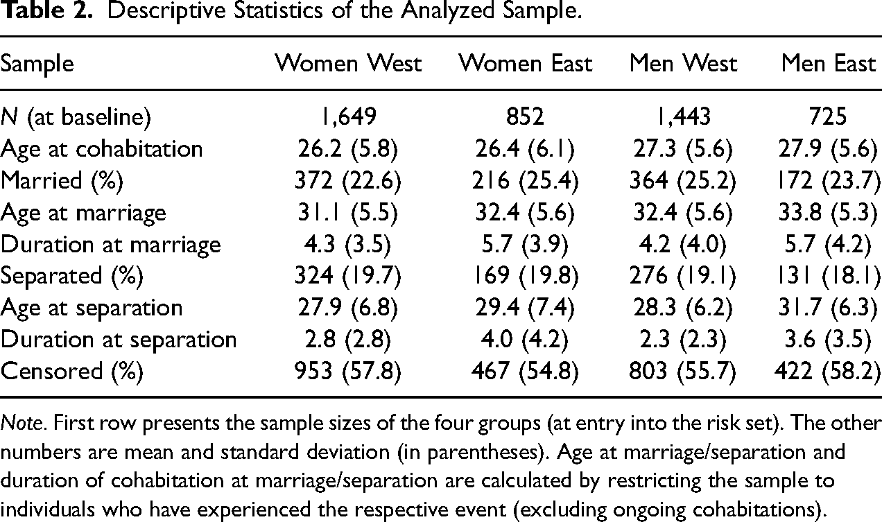
Note. First row presents the sample sizes of the four groups (at entry into the risk set). The other numbers are mean and standard deviation (in parentheses). Age at marriage/separation and duration of cohabitation at marriage/separation are calculated by restricting the sample to individuals who have experienced the respective event (excluding ongoing cohabitations).
Estimated Hazards Over two Time Scales
We present the results separately for the event “marriage” and for the event “separation,” and we compare the interaction model (8) with the simpler additive model (4) and the varying-coefficient model (6). In the analysis,
We estimate the smooth hazard of marriage or separation for each of the four groups (men/women; East/West) separately. In all models, we choose cubic
Transitions From Cohabitation to Marriage
Table 3 summarizes the optimal values of the smoothing parameters, which were obtained by minimizing AIC, the resulting effective dimensions, and the values of AIC for the twelve models. In each case, the smallest AIC is marked in bold.
Hazard of Marriage.
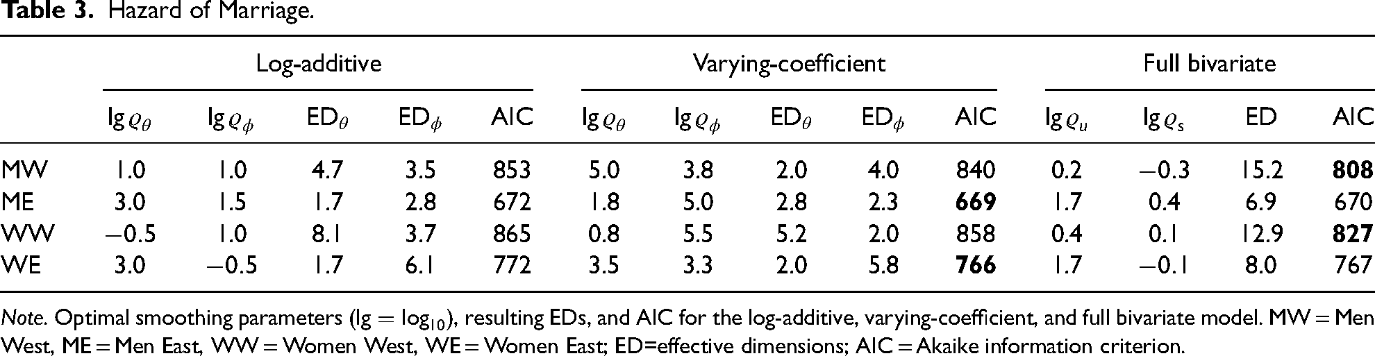
Note. Optimal smoothing parameters (
In all four groups, a log-additive (proportional hazards) model is too simple. A single hazard shape over
Figure 4 shows the estimated surfaces of
Hazard of marriage over age at entry into and duration of cohabitation: Comparison of the log-additive model (left), varying-coefficient model (center), and 2D interaction model (right) for Men West (top) and Men East (bottom). Corresponding values of effective dimensions and AIC are in Table 3.
Hazard of marriage over duration of cohabitation for selected values of age at entry into cohabitation (
In general, hazard levels for marriage are lower in East Germany than in West Germany, confirming previous research. For West German men, there is a noticeable increase in the hazard for cohabitations that start between ages 25 and 30 and end, due to marriage, after about five years (see top right panel). For cohabitations that are entered at later ages, marriage rates also peak at about four to five years, although at lower levels. Also, there is an increase in the marriage hazard for individuals who started cohabiting quite young (and did not split up) with increasing duration of their cohabitation, peaking at about 10–15 years, for
For men in East Germany, the plots in the bottom row, center, and right, of Figures 4 and 5 confirm the results in Table 3: The estimates of
The estimated surfaces
Transitions From Cohabitation to Separation
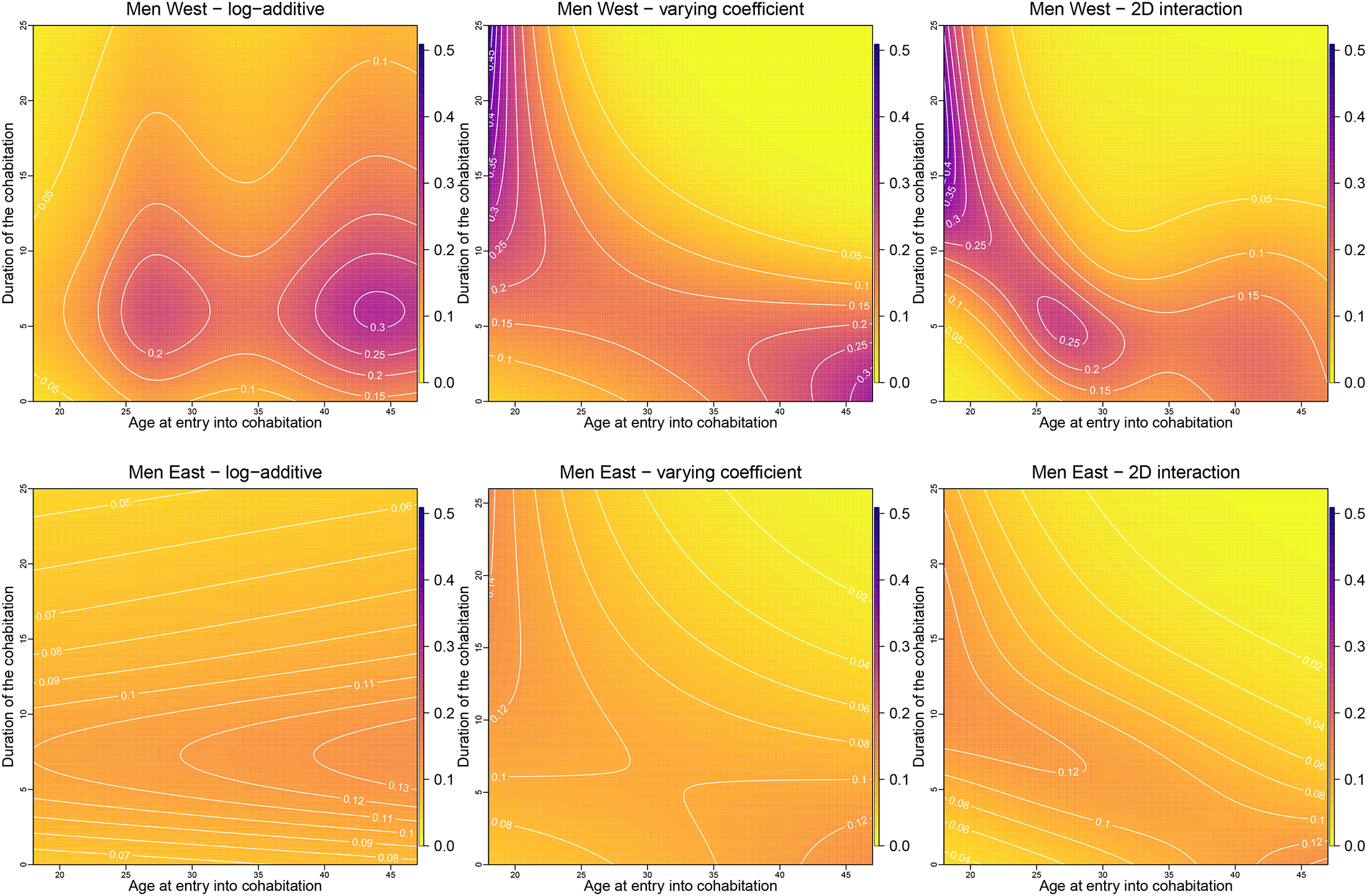
The results for the hazard of separation in the four groups are summarized in Table 4.
Hazard of Separation.
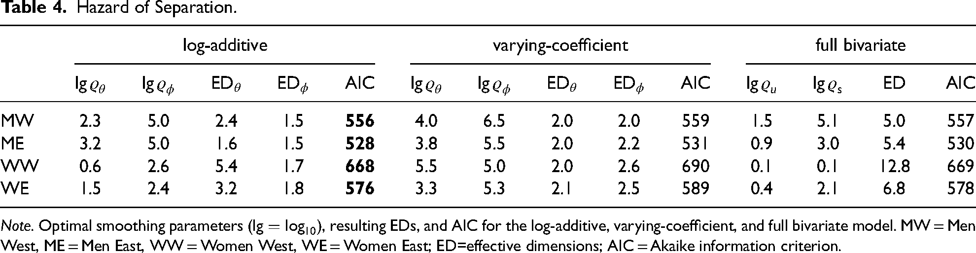
Note. Optimal smoothing parameters (
Different from the marriage rates, the conclusions here are uniform and lead to a much simpler result: In all four groups, the additive model has the smallest AIC, so a single hazard
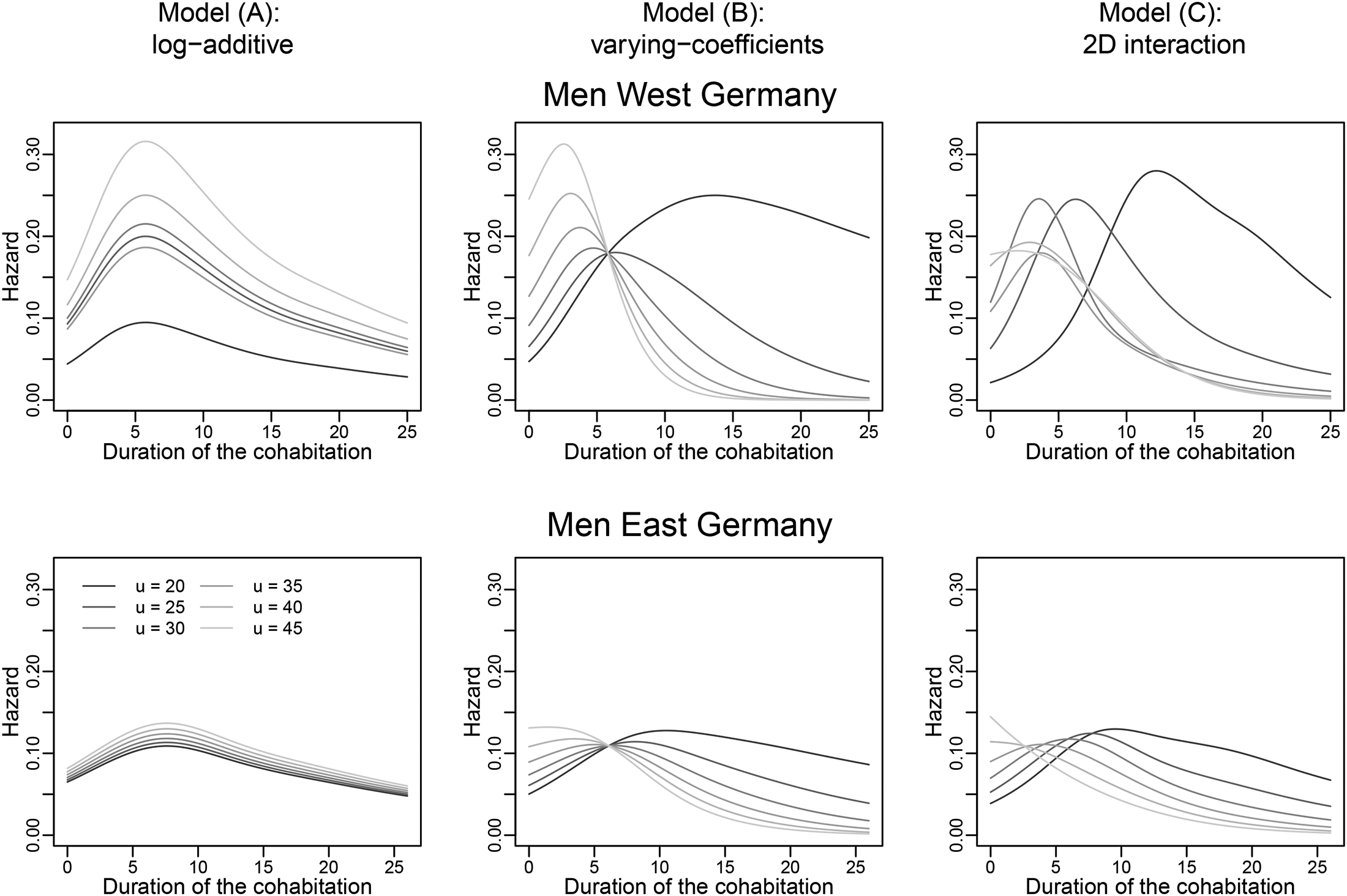
Figure 6 presents the results for men. The estimated functions
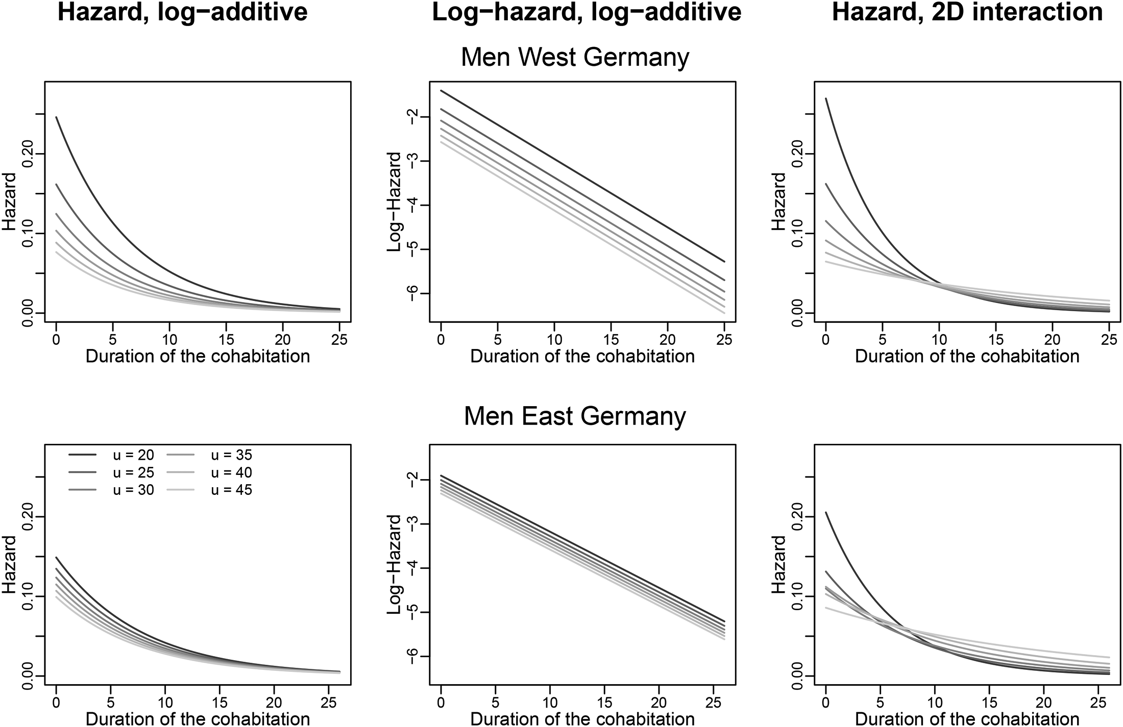
Hazard of separation over duration of cohabitation for selected values of age at entry into cohabitation (
In summary, the proposed methodology identifies quite different models for the hazard of marriage and of separation. The level of complexity ranges from a simple PH model to a full bivariate hazard surface. AIC (or BIC) provides a convenient measure for model comparison and selection, effective dimensions of the models give further useful information on the model complexity. When a simpler model is selected as optimal, then the full bivariate surface reproduces the simpler hazard.
Discussion and Outlook
When processes evolve in time, several time scales may be important, and models that are used to analyze such processes should allow us to incorporate more than one time scale. This will allow us to investigate their joint roles in the process. This paper offers an approach to incorporate multiple time scales in the analysis of time-to-event data and demonstrates its use in the study of transitions out of nonmarital cohabitation to either marriage or separation. We review how the simultaneous analysis of two time scales in hazard models can be reformulated using an “age-period-cohort”-like relationship. The impact of two time scales can then be expressed in a single time scale model with covariate effects of different complexity, ranging from a proportional hazards structure to a full bivariate hazard surface in which the covariate modulates the hazard smoothly but without additional imposed structure.
To estimate these hazard models, we suggest to use
In the application, we demonstrate how the proposed approach identifies, using a single methodology, interactions of different complexity (for the hazard of marriage) or much simpler proportional hazards (for transitions to separation), which can even be modeled parametrically.
The initial binning of the data is sometimes claimed to be a drawback even though it is this binning that was recognized, already several decades ago, to provide the extremely productive link between hazard modeling and Poisson regression. Even somewhat narrow bins that contribute to the flexibility of
Recent alternative approaches to model hazards over two time scales use flexible parametric models (Batyrbekova et al. 2022; Bower et al. 2022). Full bivariate hazard surfaces, which are required for some hazards in our application, are mentioned but, as far as we can tell, have not been implemented yet.
Our analysis of transitions from cohabitation to marriage or separation in Germany shows interesting results. Previous research, using the same data, found that the rate of marrying (or separating) steadily increases in the first five years after cohabitation and thereafter remains unchanged, and that age at cohabitation did not significantly change the hazard rates (Hiekel et al. 2015). Our results tell a more complicated story.
In this study, the focus was on assessing the impact of several time scales, and no further covariates were included. It is, however, possible to use hazards over two time scales as a baseline hazard in a proportional hazards (PH) model. The extension to the PH regression model is discussed in Carollo et al. (2025), and it is implemented in the R-package, currently only for fixed covariates. We decided to omit details about the implementation of the PH model; however, we do present the results of PH analysis in the online supplement, using the same data as in Hiekel et al. (2015), including the same covariates but using a two-dimensional baseline hazard instead. We find that, even when using the same sample and controlling for the same covariates, the baseline hazard of marriage and of separation over the duration of the cohabitation differ substantially by age at entry into cohabitation. This comparison provides evidence that differences between the two analyses may be explained by the use of the considerably more flexible hazard models, rather than differences in the analyzed sample.
Our results also show differences in the rate of marriage between East and West German men and women, which are coherent with the literature on the topic. Klarner and Knabe (2017) found that East German individuals see marriage as an institution with little relevance for everyday behavior or for the meaning of their partnerships, while Western German couples still believe in marriage as an institution, and one of the biggest arguments in favor of marriage is the formalization of the relationship.
We analyzed cohabitation from age 18 onward. To check how sensitive our results are to this choice, we repeated the analysis, enlarging our sample to ages at entry into cohabitation as low as 15 years by adding 230 cohabitations. The patterns shown in the hazard of marriage or separation remain mostly unchanged. Also, we considered one cohabitation per individual in our sample, which might not have been the first ever cohabitation experienced by the individual. It is possible that the risk of marriage or separation among first-time cohabiters is different from those who are in their second or higher cohabitation. To check if our results are robust regarding the order of the cohabitation, we ran another analysis restricting the sample to the first-ever cohabitation only, thereby removing about 25.5% of all observations. We again find that the way both time dimensions interact is the same among first-time cohabiters and among all cohabiters. Both these additional sensitivity analyses are presented in the online supplement.
The analyses presented in this paper were produced using the
The current model is limited to the inclusion of two time scales. Occasionally, additional time scales might be relevant, although we suspect that more than three time scales may challenge our power of imagination. Extension of the
We analyzed cause-specific hazards, considering the competing events of marriage and separation. From the cause-specific hazards, transition probabilities can be calculated, as shown in Carollo et al. (2024), to complete a competing risks analysis. Extensions to more complex multi-state models will be the topic of future research, too. In view of the current debate about the role that childbearing has in union formation (see, e.g., Wright 2019, Schnor 2014, and Lappegård et al. 2018) such extensions are of practical relevance. It is conceivable that with additional transitions, also additional time scales gain importance.
Supplemental Material
sj-pdf-1-smr-10.1177_00491241251374193 - Supplemental material for Analysis of Time-to-Event Data With Two Time Scales. An Application to Transitions out of Cohabitation
Supplemental material, sj-pdf-1-smr-10.1177_00491241251374193 for Analysis of Time-to-Event Data With Two Time Scales. An Application to Transitions out of Cohabitation by Angela Carollo, Hein Putter, Paul H.C. Eilers and Jutta Gampe in Sociological Methods & Research
Supplemental Material
sj-pdf-2-smr-10.1177_00491241251374193 - Supplemental material for Analysis of Time-to-Event Data With Two Time Scales. An Application to Transitions out of Cohabitation
Supplemental material, sj-pdf-2-smr-10.1177_00491241251374193 for Analysis of Time-to-Event Data With Two Time Scales. An Application to Transitions out of Cohabitation by Angela Carollo, Hein Putter, Paul H.C. Eilers and Jutta Gampe in Sociological Methods & Research
Footnotes
Acknowledgments
We are very grateful to Nicole Hiekel from the Max Planck Institute for Demographic Research for her helpful comments on an earlier version of this manuscript. Her insights greatly helped to shape the presentation of the application and discussion of the findings. This paper uses data from the German Family Panel pairfam, coordinated by Josef Brüderl, Sonja Drobnič, Karsten Hank, Bernhard Nauck, Franz Neyer, and Sabine Walper. pairfam is funded as a long-term project by the German Research Foundation (DFG).
Declaration of Conflicting Interests
The authors declared no potential conflicts of interest with respect to the research, authorship, and/or publication of this article.
Funding
The authors received no financial support for the research, authorship, and/or publication of this article.
Preregistration Statement
This study was not preregistered.
Supplemental Material
Supplemental material and Appendix for this article are available online.
Data and Code Availability Statement
The data were used under license from GESIS for the current study and are not publicly available. However, the data can be accessed using the instructions provided here: https://www.pairfam.de/en/data/data-access/. The code used for this study and documentation for the code are available in the GitHub repository (Carollo, 2025) indexed with Zenodo 1 .
Notes
Author Biographies
References
Supplementary Material
Please find the following supplemental material available below.
For Open Access articles published under a Creative Commons License, all supplemental material carries the same license as the article it is associated with.
For non-Open Access articles published, all supplemental material carries a non-exclusive license, and permission requests for re-use of supplemental material or any part of supplemental material shall be sent directly to the copyright owner as specified in the copyright notice associated with the article.