Sage Journals: Discover world-class research

Abstract

In the wake of the methodological developments that aim to render qualitative comparative analysis (QCA) “time sensitive”, I propose a new procedure for carrying out QCA longitudinally. More specifically, I show first why longitudinal case disaggregation should be carried out with change-based intervals (CBIs) rather than with fixed intervals. Second, I develop a flexible lag condition (FLC) that (i) resolves two types of temporal contradictions and outcome redundancies that can result from temporal case disaggregation and (ii) allows to measure the average duration it takes for a combination of conditions to translate to an outcome. Since temporal contradictions and outcome redundancies are most likely with an increasing number of time points and conditions, as well as with CBIs in general, the FLC procedure is most useful in these cases. The fact that the interest of longitudinal analyses increases with the number of disaggregated cases underlines the usefulness of the proposed methodological innovation. Despite its suitability for mid-n and large-n analyses, longitudinal QCA with an FLC preserves a strong case-oriented and qualitative perspective and remains thereby loyal to QCA's original foundations.

Keywords

QCA set-theoretic methods longitudinal analyses CBIs FLC comparative methods.

Introduction

Qualitative comparative analysis (QCA) is a case-based “set-theoretic” method that uses Boolean logics of “necessity” and “sufficiency” to systematically compare in the presence or absence of which (combinations of) “conditions” an “outcome” is present or absent. Being initially conceived as a static method of analysis, an increasing methodological scholarship has proposed ways to account for temporal variation in QCA. In the wake of these developments, I propose a new procedure for carrying out QCA longitudinally with two core ideas. First, I disaggregate cases in their temporal development stages each time a change occurs in one of the conditions or the outcome under study. I call this change-based intervals (CBIs). Second, I use a flexible lag condition (FLC) to resolve the temporal contradictions and outcome redundancies that can result from temporal case disaggregation. Doing so, the FLC allows furthermore to measure the average duration it takes for a combination of conditions to translate to an outcome.

The QCA procedure that was developed originally by Ragin (1987) has been refined since then by a growing methodological community and relies on three main steps (to go further, see Rihoux and Ragin (2009) and Schneider and Wagemann (2012), on which I draw for the summary below). First, one determines which value cases take in each condition and the outcome of interest. Conditions and outcomes are calibrated as “sets” and differ from variable-oriented approaches in that, rather than measuring absolute degrees of a phenomenon, they capture the relative extent to which a phenomenon is present or absent in a case. Conditions can be calibrated dichotomously (presence vs. absence) as “crisp sets”, they can be calibrated with differentiations in both degree and kind (degrees of presence vs. degrees of absence) as “fuzzy sets”, or they can account for different conceptual levels (type 1 vs. type 2 vs. type 3) as “multi-value sets”. Second, all cases with identical values for the conditions and the outcome are grouped in a “truth table” as “configurations”. Doing so, cases who share the same properties are considered jointly and the analytical attention shifts from cases to configurations. In this step, all configurations should lead to the same outcome (either the presence or absence of the phenomenon). Otherwise, one is presented with contradictory evidence and so-called “contradictory configurations” (or “contradictory/inconsistent truth table rows”) need to be resolved before the analyses can be carried out. Third, Boolean logics are used to determine which (combinations of) conditions are necessary and which are sufficient for the outcome to occur (and which are for it not to occur). In the analysis of sufficiency, combinations are “minimized” in order to avoid “logical redundancies” and only comprise conditions that are necessary for the combination to be sufficient in explaining the presence or absence of the outcome.

QCA has three epistemological characteristics. It has a constellational view of causality in that it explicitly looks for the combinations of conditions (linked by a logical conjunction [and] or disjunction [or]) under which an outcome is present or absent. It has an “equifinal” view of causality in that it conceives different (combinations of) conditions as equally capable of producing the same outcome. It has an asymmetrical view of causality in that it does not assume the absence of an outcome to be explained by the negation of what explains its presence.

While QCA was initially conceived as a static method of analysis (Ragin 1987) without explicit account for the temporal order of conditions or for the variation of cases over time (Boswell and Brown 1999:181, Schneider and Wagemann 2012:80), a growing number of methodological innovations has been developed to render QCA time sensitive (Furnari 2018). The first strand of innovations is condition-focused in that they either account for the temporal sequence of conditions (Caren and Panofsky 2005, Hak, Jaspers and Dul 2015, Ragin and Strand 2008) or process QCA in two steps as to distinguish contextual “remote” conditions from agency-oriented “proximate” conditions (Schneider 2019). The second strand is case-focused and suggests how to use QCA longitudinally, i.e., with temporally disaggregated cases. They provide calibration mechanisms for time series QCA (Hino 2009), adapt traditional consistency measurements for panel data QCA (Garcia-Castro and Ariño 2016), or propose different ways to account for and trace within-case changes over time (Pagliarin and Gerrits 2020, Verweij and Vis 2021).

In this article, I aim to further develop this second strand. While its existing works clearly improve the ability of QCA to integrate various aspects of time, they remain silent on (i) how to best disaggregate cases temporally in their development stages and (ii) how to deal with the contradictory and redundant configurations that can arise from temporally disaggregated cases. I argue that cases in longitudinal QCA should be disaggregated based on changes in the characteristics of the case—i.e., when cases’ membership in a condition or the outcome under study change either in degree or in kind—rather than based on fixed intervals. I call these “change-based intervals” (CBIs). While superior in both conceptual and empirical terms, CBIs increase the chance for two types of temporally contradictory configurations. These are contradictions that come with the temporal disaggregation of cases rather than with traditional empirical contradictions. In parallel, CBIs also increase the chance for redundant outcome configurations, which are outcome configurations with empirically identical information. To address these issues, I developed what I call a “flexible lag condition” (FLC). It offsets the temporal contradictions and redundancies, and accounts for the average duration it takes for a (combination) of conditions to be present before the outcome occurs.

To develop on these suggestions, I proceed as follows in this article. In the first section, I explain why I think that case disaggregation in longitudinal QCA should follow changes in the characteristics of a case. In the second section, I show why this increases the chance of temporal contradictions and outcome redundancies among the disaggregated case distribution. In the third section, I present the rationale and usefulness of the FLC to resolve the aforementioned contradictions and redundancies, and illustrate its use in a minimal analysis with a crisp set example. I then discuss how the procedure could be extended to fuzzy set and multi-value QCA, as well as the potential pitfalls of my suggestion—notably the risk for hiding an omitted condition, the risk for outcome-skewness, and the need for a modified algorithm to obtain the intermediate and most parsimonious solutions. I conclude with a discussion of the main contributions to and compatibility with existing methodological innovations that aim to render QCA time sensitive.

Why to Prefer CBIs Over Fixed Intervals

In longitudinal QCA, there are two ways to disaggregate cases temporally into their development stages—as alluded to by De Meur, Rihoux and Yamasaki (2009:162). On the one hand, one can disaggregate them in fixed intervals (e.g., every year, every 5 years, every 10 years, etc.). The rationale behind this is to consider change as inherently temporal and to look for potential evolutions of a case in regular periods that are not dependent on the case itself. Instead, cases are conceived as empirical realities to be observed at different regular points in time that deserve to be considered distinctly because of the very temporal advancement.

On the other hand, on can disaggregate them based on changes in the characteristics of the case. That is when a case changes its membership in a condition or the outcome under study either in degree or in kind. I call this “change-based intervals” (CBIs). The rationale behind this is to consider change as enabled by time but as dependent on evolutions of the relevant characteristics of the case itself. Cases are then conceived as empirical realities whose development stages are only to be considered distinctly when one of its relevant characteristic changes, i.e., either its membership in one of the conditions or the outcome. Such changes should not only be captured in kind but also in degree because even if the latter do not alter the overall presence or absence of a condition in a case, they consist in a new empirical reality and furthermore lead to different parameters of fit.

Despite these differences between the two approaches, one should note that they both consider the different development stages of a case as separate units of observation. This is an important methodological choice that needs to be justified and reflected in the interpretation of the analysis (Goertz 2017, Ragin 1992). Put differently, while in traditional static QCA, we consider “cases” as both units of observation and analysis, we are presented here with two different types of units: “development stages”, which take the role of units of observation; and “cases”, which remain the higher-order unit of analysis at which conclusions are drawn at the end of the study.

There are three reasons why I think that CBIs are to be preferred over fixed intervals when carrying out longitudinal QCA. First, it prevents different condition realities from falling within a single interval, leading to measurement inaccuracy. When the condition or outcome properties of a case do change at the middle of a fixed-interval, the researcher has to choose if the properties are considered different since the beginning of the interval during which they changed or only since the beginning of the subsequent one. Both choices comprise some degree of inaccuracy and can lead to anachronisms when several conditions and/or the outcome change during the same interval.

When conditions and the outcome are calibrated as to account for their change from one interval to the other, as in Hino's (2009) “time differencing” QCA, empirical changes at the middle of a fixed interval might seem less problematic because one is interested in degrees of change over time rather than in effective scores. However, this might also lead to anachronisms when changes in a condition and the outcome occur at different moments of the interval (e.g., when in a 5-year interval, the outcome changes in year 2 but the condition only in year 4). Furthermore, when more than one change occurs in a single interval, both direct- and time differencing calibration mechanisms are unable to reflect it in fixed intervals.

Second, and related to the previous point, CBIs reflect accurately the moment in which empirical realities change. By disaggregating cases each time that the properties of a case change for either a condition or the outcome, one provides a precise picture of the empirical case realities throughout time and prevents anachronisms because the anteriority, simultaneity, and posteriority of changes are correctly captured.

Third, CBIs avoid what could be considered as empirical redundancies over several intervals because it only disaggregates cases when they empirically evolve. In fixed intervals, cases can be disaggregated into different development stages even when no condition or the outcome change, i.e., a case is disaggregated without presenting a new empirical reality. Unless one considers that these intervals deserve to be considered distinctly by virtue of the very temporal advancement, one is just presented with empirically identical cases. Since this increases the number of cases, it also impacts necessity and sufficiency parameters. For example, if they are confirming or contradicting cases for a path, they influence the consistency of sufficiency (and coverage of necessity) scores. If they are uncovered by a path, they influence coverage of sufficiency (and consistency of necessity) scores. These scores can be considered distorted if such a disaggregation is not justified.

The three reasons above rely on the assumption that the temporal change of the conditions and outcome under study is irregular—which I expect to apply to the vast majority of research problems in the humanities. When condition-change should nevertheless be regular, CBIs will simply equal fixed intervals because the change-based disaggregation will coincide with the regular condition change. I maintain thus that CBIs are preferable in any research problem because they can only improve but not worsen the empirical observation.

The aforementioned methodological innovations on longitudinal QCA have illustrated their procedure with cases that have been disaggregated based on fixed intervals. In his example of the three ways to calibrate time series QCA, Hino (2009) went with 10-year intervals. Garcia-Castro and Ariño (2016), developed their pooled, within and between consistency measurements based on fixed annual intervals. Pagliarin and Gerrits (2020), in turn, used Hino's (2009) example for their own illustration of a trajectory-based QCA. However, they grouped identical configurations and made clear that their procedure also works with “different time-specific development stages” (8)—which corresponds to CBIs. Verweij and Vis (2021), finally, develop their three propositions to track evolving case configurations over time with 5- and 10-year intervals. While all these propositions make valuable contributions to the integration of time in QCA, I would strongly encourage their future applications to reflect on the choice between CBIs and fixed intervals in light of the arguments above, especially because they are all compatible with CBIs.

A consequence of existing longitudinal QCA methods being developed and illustrated with fixed intervals, however, is that little attention has been dedicated to the problem of temporally contradictory configurations arising from temporally disaggregated cases. As I show in the next section, such contradictions are more likely with (although not limited to) CBIs. Furthermore, the likelihood of temporal contradictions increases with the number of temporal disaggregations as well as with the number of conditions included in the analysis. While the illustration of Hino (2009) (and that of Pagliarin and Gerrits (2020) who replicate it for their method) are based on a case disaggregation with only two time points, that of Verweij and Vis (2021) is based on four. The analysis of Garcia-Castro and Ariño (2016) involves 10 annual points but includes only a single condition. Taken together, these three elements hint to why temporally contradictory configurations were not yet on the radar of my precursors—in addition to the fact that QCA is a comparatively young method, certainly when used longitudinally. Since the interest of longitudinal research increases with the number of disaggregated cases and conditions (Gerrits and Pagliarin 2021), I developed a method that helps overcoming the temporal contradictions they cause.

The Problem of Temporal Contradictions and Redundant Outcomes in Longitudinal QCA

When carrying out a longitudinal QCA, one can run into the problem of two types of “temporally contradictory configurations”, i.e., configurations that are associated both with the presence and the absence of the outcome.¹ I call these contradictions “temporal” because they come with the temporal disaggregation of cases and conditions’ insensitivity for time rather than with classical empirical contradictions, as I argue below. Table 1 shows a theoretical example of five main cases that have been disaggregated temporally based on the changes of four conditions (A, B, C, D) and the outcome (O). Doing so, the amount of temporally disaggregated cases equals 18. The conjunctions A*B and A*C will appear to be sufficient for the outcome in the illustrative analyses conducted below. I use them already here to illustrate the two types of temporal contradictions.

Table 1.

Theoretical Example of the two Types of Temporal Contradictions and Outcome Redundancies.

Cases	From	To	Conditions				Outcome	Temporal contradictions
			A	B	C	D		For A*B		For A*C		For A*B	For A*C
			A	B	C	D		Time-ins.	Emp. red.	Time-ins.	Emp. red.	For A*B	For A*C
Case 1	1920	1945	0	0	0	1	0
Case 1	1946	1950	1	1	0	0	0	⬤
Case 1	1951	1955	1	1	0	0	1	⬤				⬤
Case 1	1956	1964	1	1	0	1	1					⬤
Case 2	1912	1961	0	1	1	1	0
Case 2	1962	1972	1	0	1	0	0			⬤
Case 2	1973	1977	1	0	1	0	1			⬤			⬤
Case 2	1978	1982	1	0	1	1	1						⬤
Case 3	1933	1959	0	0	1	1	0
Case 3	1960	1985	0	1	1	0	0
Case 3	1986	1989	1	1	1	0	1					⬤	⬤
Case 3	1990	1993	1	1	1	1	1					⬤	⬤
Case 4	1940	1945	1	0	1	0	0				⬤
Case 4	1946	1951	1	0	1	1	0			⬤	⬤
Case 4	1952	1952	1	0	1	0	1			⬤
Case 5	1926	1937	0	0	0	0	0
Case 5	1938	1963	1	0	1	1	0				⬤
Case 5	1964	1970	1	0	1	0	0				⬤

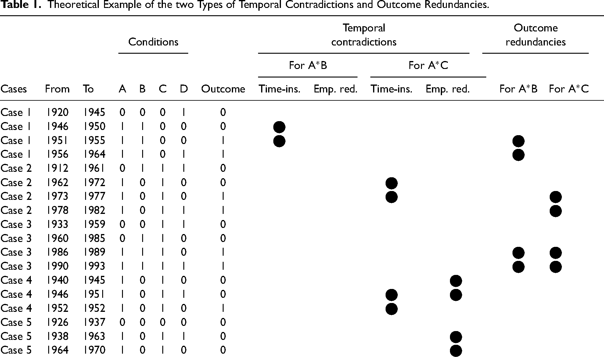
The first type of temporal contradictions that can be called “time insensitive”, arises when the configuration leading to the presence of the outcome is identical to the temporally preceding configuration, except for the outcome which is absent. I call this kind of contradiction “time insensitive” because it can be due to the omission of time as a condition in itself, i.e., that a certain combination of conditions needs time before translating into an outcome (as discussed below, the omission of time is not to be confounded with the omission of another condition itself). In the theoretical example as shown in Table 1, this happens for the conjunction A*B in Case 1 (1946–1950; 1951–1955) and for the conjunction A*C in Case 2 (1962–1972; 1973–1977) as well as in Case 4 (1946–1951; 1952–1952). In Case 3 (1986), the condition change for both the conjunction A*B and A*C is immediately accompanied by the occurrence of the outcome, i.e., that there is no temporal contradiction. In Case 5, the outcome does not occur.

The second type of temporal contradictions that can be called “empirically redundant”, arises when the number of contradicting configurations is increased by identical configurations that follow on each other but are not grouped—either because they are repeated in fixed interval disaggregation, or because they are separated in CBI disaggregation by a condition that is not necessary for a combination of conditions to be sufficient for the outcome.² I call this kind of contradiction “empirically redundant” because it relies on configurations that are identical with respect to the conditions in the conjunction. This holds for both CBIs and fixed intervals, unless one can convincingly argue that the latter deserve to be considered distinctly by virtue of the very temporal advancement (see discussion above). In the example in Table 1, this happens for the conjunction A*C in Case 5 (1938–1963; 1964–1970). Since B and D are minimized and not relevant for A*C, instead of two contradictory development stages for Case 5 (1938–1963; 1964–1970), there should be only one (1938–1970). In Case 4, there are also two empirically redundant development stages (1940–1945; 1946–1951) for the conjunction A*C that should be grouped. They are, however, not contradictions strictu sensu because they equal the last development stage whose time-insensitive contradiction will be resolved by the FLC in the analysis below.

Finally, there is not only the possibility of temporally contradictory configurations, but also that of “empirically redundant outcome configurations”. Like empirically redundant contradictions (the second contradiction type), they can stem from the disaggregation of cases based on fixed intervals or from CBI disaggregation by a condition that is not necessary for a combination of conditions to be sufficient for the outcome. They are “empirically redundant” because they rely on configurations that are identical with respect to the conditions in the conjunction. They are not contradictions, however, because they do not contradict the instance in which the configuration leads to the outcome. Instead, they actually increase the number of confirming cases. Since they do so artificially (unless one can convincingly argue that the stages deserve to be considered distinctly by virtue of the very temporal advancement, as discussed above), I also suggest to offset them for the calculation of the parameters of fit (see below).

When reflecting on the likelihood of these two types of contradictions and outcome redundancies, I cannot make a statistical evaluation in the absence of a sufficient number of existing applications. However, the following reflections lead me to expect that CBIs are more likely to produce both temporally contradictory configurations and outcome redundancies than fixed intervals. Time-insensitive contradictions (type 1) are likely in change-based disaggregation because a change in the outcome creates by definition a new configuration. A contradiction between the outcome configuration and the last configuration then arises unless a change in one condition of the preceding configuration occurs exactly at the same point in time. With fixed intervals, this kind of disaggregation is possible when intervals and empirical changes coincide. But it seems less likely otherwise because multi-annual intervals can be coded in such a way that condition and outcome changes fall in the same interval. As for empirically redundant contradictions (type 2) and outcome redundancies, if one considers that all conditions under study are seldomly necessary in all paths (and even the solution) of a QCA, it is very likely that conditions that are neither sufficient on their own, nor necessary in a sufficient combination of conditions (INUS) will contribute to change-based case disaggregation and thereby artificially increase the number of contradicting configurations or outcome configurations. With fixed intervals, case disaggregation is not dependent on such conditions. They rather come with the risk of multiplying identical configurations (see above).

There are two more factors that influence the likelihood of temporal contradictions and outcome redundancies, and they hold equally for CBIs and fixed interval disaggregation. Both (i) the number of disaggregated periods and (ii) the number of conditions included in the analysis influence the number of configurations that can be contradicting and ungrouped—both for the configuration preceding the one that leads to the outcome (impacting the likelihood of time-insensitive contradictions), and for all other configurations (impacting the likelihood of empirically redundant contradictions).

Now, one might want to argue that what I call time-insensitive contradictions (type 1) are legitimate because a change in the outcome should be accompanied by a change in at least one condition for a meaningful relationship between a combination of conditions and the outcome to be established. This would indeed be the ideal scenario. However, this purist interpretation omits time as a crucial condition in itself. For some combination of conditions to translate into a change in the outcome, a certain amount of time might indeed be needed without any other change in the combination. That being said, before the conclusion can be reached that time is the omitted condition, the existence of another omitted condition needs to be considered—either theoretically or through further in-depth examination of the cases—and ruled out. As for empirically redundant contradictions (type 2) and outcome redundancies, unless one can convincingly argue that the different development stages need to be considered distinctly by virtue of the very temporal advancement (see discussion above), I see little ground for them to be justified if they just result from the disaggregation based on conditions that are irrelevant for the outcome.

To my knowledge, there is only one theoretical suggestion and one recent application that partially addresses the problem of time insensitivity. In their reflection on how to analyze policy processes with QCA, Fischer and Maggetti (2017) propose five ways to “address the challenge of temporality” (10–12). One of them consists in accounting for time with a separate condition that distinguishes between younger and older cases. In their research on the best performing business model in Formula One racing between 2005 and 2014, Aversa, Furnari and Haefliger (2015) go in this direction too and avoid what I called type 1 contradictions by analyzing data separately on a biannual basis and then using a 1-year lag. This idea of fixed lag goes in the right direction and might be suitable for analyses of short absolute time frames in an area with rapid and regular changes. For the study of longer time frames and irregular changes like in most of the research in the humanities, however, a fixed lag proves problematic because the required amount of time to be accounted for is variable. This is the reason for why I propose to use a flexible lag whose time frame is determined by the changes of cases’ membership in the conditions and the outcome under study.

How to Resolve Temporal Contradictions and Redundancies with a FLC

Rationale

To account for time as an omitted condition and group identical configurations through a FLC, three things are needed, as shown by the example in Table 2.

Table 2.

Theoretical Example of the Flexible Lag Conditions (FLCs) for A*B and A*C and Their Conjunctions.

Cases	From	To	Conditions				Outcome	A*B			A*C
Cases	From	To	A	B	C	D	Outcome	FLC_w/oor	ABFLC_w/oor	Lag	FLC_w/oor	ACFLC_w/oor	Lag
Case 1	1920	1945	0	0	0	1	0	1	0	-	1	0	-
Case 1	1946	1950	1	1	0	0	0	0	0	-	0	0	-
Case 1	1951	1955	1	1	0	0	1	1	1	5	1	0	-
Case 1	1956	1964	1	1	0	1	1	0^a	0	-	0^a	0
Case 2	1912	1961	0	1	1	1	0	1	0	-	1	0	-
Case 2	1962	1972	1	0	1	0	0	0	0	-	0	0	-
Case 2	1973	1977	1	0	1	0	1	1	0	-	1	1	11
Case 2	1978	1982	1	0	1	1	1	0^a	0	-	0^a	0	-
Case 3	1933	1959	0	0	1	1	0	1	0	-	0	0	-
Case 3	1960	1985	0	1	1	0	0	1	0	-	1	0	-
Case 3	1986	1989	1	1	1	0	1	1	1	0	1	1	0
Case 3	1990	1993	1	1	1	1	1	0^a	0	-	0^a	0	-
Case 4	1940	1945	1	0	1	0	0	0	0	-	0	0	-
Case 4	1946	1951	1	0	1	1	0	0	0	-	0	0	-
Case 4	1952	1952	1	0	1	0	1	1	0	-	1	1	12
Case 5	1926	1937	0	0	0	0	0	1	0	-	1	0	-
Case 5	1938	1963	1	0	1	1	0	0	0	-	0	0	-
Case 5	1964	1970	1	0	1	0	0	1	0	-	1	1	-

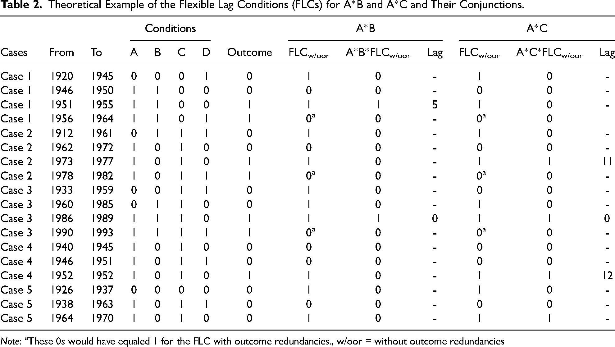
Note: ^aThese 0s would have equaled 1 for the FLC with outcome redundancies., w/oor = without outcome redundancies

First, instead of grouping identical configurations in a frequency-based truth table like in traditional QCA, the development stages of temporally disaggregated cases need to be ordered in a chronological data matrix (e.g., Case 1 (1920–1945), Case 1 (1946–1950), Case 1 (1951–1955), etc.). This allows identical combinations of conditions that directly follow on each other in the same disaggregated case to be considered jointly (see next point).

Second, a lag condition needs to capture each change in either the combination of conditions or the outcome under study. This means that it has to equal 1 for the last row of a series of identical combinations of conditions, as well as when the outcome occurs, such that: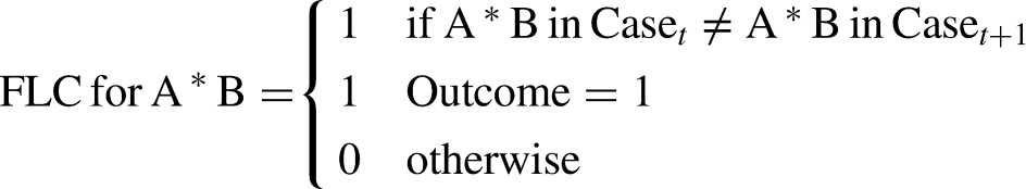

FLC for A * B = {\begin{matrix} 1 & if A * B in Cas e_{t} \neq A * B in Cas e_{t + 1} \\ 1 & Outcome = 1 \\ 0 & otherwise \end{matrix}

If this lag condition is also supposed to offset empirically redundant outcome configurations, it should only equal 1 for outcomes that are not repeated for the same combination of conditions, such that:

\begin{aligned} FL C_{\binom{w / o}{\binom{o u t c .}{r e d .}}} for A * B = & {\begin{matrix} 1 & if A * B in Cas e_{t} \neq A * B in Cas e_{t + 1} \\ 1 & if Outcome = 1^{^} A * B in Cas e_{t} \neq A * B in Cas e_{t - 1} \\ 0 & otherwise \end{matrix} \end{aligned}

The rationale behind the lag is twofold. (i) Since it only equals 1 at the end of a series of similar combinations of conditions for which it was calculated, the conjunction between the lag and the conditions for which it was calculated only considers one instance of identical combinations of conditions if they have previously been separated by an unnecessary condition for sufficiency. This avoids empirically redundant contradictions. In the example as shown in Table 2, the lag for A*C does this for Case 4 (1940–1945; 1946–1951) and Case 5 (1938–1963; 1964–1970) since the distribution of A*C is identical for them. The lag variant without outcome redundancies applies the same logic to empirically redundant outcome configurations, where only the first of otherwise identical outcome configurations is taken into consideration. In the example as shown in Table 2, the lag for A*B does this for Case 1 (1951–1955; 1956–1964) and Case 3 (1986–1989; 1990–1993). The lag A*C does this for Case 2 (1973–1977; 1978–1982) and Case 3 (1986–1989; 1990–1993).

(ii) Since the lag equals 1 for every first occurring outcome, the conjunction between the lag and the conditions for which it was calculated lags the occurrence of the outcome vis-à-vis the previous combination of these conditions if it is identical. This resolves time-insensitive contradictions coming with the fact that a combination of conditions might need time to translate into the outcome. In Table 2, for example, the lag for A*B lags Case 1 (1951–1955) vis-à-vis the preceding Case 1 (1946–1950) whose combination of A*B is identical but where the outcome is not yet present. The same hold for the lag of A*C which lags Case 2 (1973–1977) vis-à-vis Case 2 (1962–1972), and Case 4 (1952–1952) vis-à-vis Case 4 (1940–1945; 1946–1951). As for Case 3 (1986–1989), neither the lag for A*B nor the lag for A*C had to lag it because it the occurrence of the outcome and the changes in A*B and A*C were simultaneous.

Third, the amount of time between the starting point of a combination of conditions and the occurrence of an outcome can be measured. In Table 2, for example, we see that A*B took 5 years to translate into the outcome in Case 1 (1951–1955), while the change was immediate in Case 3 (1986–1989). A*C, in turn, took 11 years to translate into the outcome in Case 2 (1973–1977) and 12 years in Case 4 (1952–1952), while the change in Case 3 (1986–1989) was also immediate. This complements the standard consistency and coverage information provided by a QCA with a specification on how much time is needed for a combination of conditions to translate into an outcome. In order to assess both the average duration and its variability, I suggest to calculate the mean and the standard deviation of the temporal lag as additional parameters of fit.

I call this condition a “lag”, because it groups identical combinations of relevant conditions across time and accounts for the duration they need to translate into the outcome. I call it “flexible” because it can take different values depending on the case—allowing (social) change to be irregular. That the FLC follows changes in the combination of conditions and not only in the outcome is absolutely crucial because it prevents it from becoming a tautology. Indeed, in Case 5 (1964–1970) in Table 2, for example, the lag of A*C equals 1 even if the outcome (O) did not occur because the development stages of A*C come to an end. We have thus a contradictory case for A*C*FLC → O, proving that it is not a tautology.

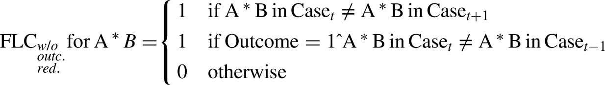
In fine, one might wonder why two different variants of the lag—one with and one without outcome redundancies—are proposed here. I have shown in the previous section that outcome redundancies artificially increase the number of confirming cases when they result from CBIs, because their disaggregation results from a condition that is not necessary for a combination of conditions to be sufficient for the outcome (the exception being if fixed intervals disaggregation can be duly justified). Because increasing the number of confirming cases influences the parameters of fit (increasing both consistency and coverage of sufficiency), I argue that their calculation should be done without outcome redundancies, i.e., based on the FLC without outcome redundancies. For the logical minimization, however, these configurations provide useful information because they show indeed that an outcome can occur regardless of the non-necessary condition for sufficiency. For the minimization, I thus suggest using the FLC that includes outcome redundancies.³

Illustrated Minimal Procedure of the Analysis

To show how the rationale above can be applied concretely in a QCA, I suggest a minimal six steps procedure that I illustrate with the theoretical crisp set example above. As specified below, the procedure can at this stage only achieve the conservative solution because the intermediate and most parsimonious solutions would require a different minimization algorithm that matches minimized conditions with the correct lag. Conceptually, however, they same logic could be applied and will hopefully in the future also be available for the intermediate and most parsimonious solutions.

A summary of the protocol can be found in Table 3. Steps 1–2 are dedicated to the analysis of necessity. Steps 3–6 are dedicated to the analysis of sufficiency. Software wise, I illustrate the analysis in R (R Core Team 2022, version 4.2.1), for which I developed eight functions that can be used to facilitate the procedure. The functions’ description, content, and arguments are summarized in the online Appendix 1. The R code for the illustrative analysis of the minimal example is provided in the online Appendix 2.

Table 3.

Minimal Protocol for a Longitudinal Qualitative Comparative Analysis (QCA) with a Flexible lag Condition (FLC).

I. Data preparation
Step 0:	Create a chronologically ordered data matrix with temporally disaggregated development stages of cases, indicating their membership in the conditions under analysis and the outcome, with unique case labels and period indications for the development stages.
II. Analysis of necessity
Step 1:	Calculate the consistency of necessity for all (combinations of) conditions. Retain those achieving at least 0.900.
Step 2:	Generate separate chronological data matrices for all (combinations of) conditions retained in step 1. Calculate the relevance of necessity for each of them and retain those achieving at least 0.500. Inspect necessity plots visually to confirm the necessity relation.
III. Analysis of sufficiency
Step 3:	Calculate the FLCs with and without outcome redundancies for all conditions under analysis, and add them to the chronologically ordered data matrix.
Step 4:	Create a truth table based on the conditions under analysis and their FLC with outcome redundancies. Proceed to the minimization (to achieve the conservative solution) and in the obtained paths, retain only the FLC that can logically be associated with the minimized path.
Step 5:	Calculate all parameters of fit for all obtained paths. Check them and only retain those achieving satisfactory consistency, do not rely (on too many) cases who deviate in kind, do not rely on simultaneous subset relations and are empirically relevant. Check the FLC of each retained path and examine whether it could correspond to an omitted condition other than time—restart the analysis if such a condition is found and include it.
Step 6:	For the eventually retained paths, calculate all parameters of fit for the solution term. Interpret the results of the paths and the solution according to traditional QCA practices.

Step 0. To have a dataset that is suitable for a longitudinal QCA with a FLC, create a chronologically ordered data matrix in which cases are disaggregated temporally in their development stages.⁴ Cases should have a common unique label (e.g., column “cases” in Table 2), while their development stages should be indicated through a coherent period indication (e.g., columns “from” and “to” in Table 2). Membership in the conditions and the outcome need to be specified for each development stage. In line with the argument made in the Introduction, the temporal case disaggregation should be change-based unless there is a specific justification for fixed intervals. After import, the CBI disaggregation can be achieved with the function CBI.df (see the online Appendix A.1.1).

Step 1. Calculate the parameters of necessity for all (combinations of) conditions. The function CBI.AoN can be used for that (see the online Appendix A.1.2). Retain—at first—all (combinations of) conditions that achieve a consistency of necessity of at least 0.900. In my theoretical example, this is the case for condition A (Cons.Nec.: 1.000, RoN.: 0.455).

Step 2. For each (combination of) condition(s) passing this threshold, calculate the parameters of necessity based on a separate chronological data matrix whose CBI disaggregation takes only into consideration changes in the outcome and in the (combination of) conditions for which the necessity test was conducted. This can again be achieved with the function CBI.AoN. If the disaggregation would also take other conditions into account, this would generate empirical redundancies that distort the relevance of necessity (RoN) score (as calculated by Schneider and Wagemann (2012:236)). For each (combination of) condition(s), retain those achieving an RoN score of at least 0.5 and satisfying a visual inspection as suggested by Oana, Schneider and Thomann (2021:64–85). In my theoretical example, this is the case for condition A (Cons.Nec.: 1.000, RoN.: 0.500) that I hence consider necessary for the presence of the outcome.

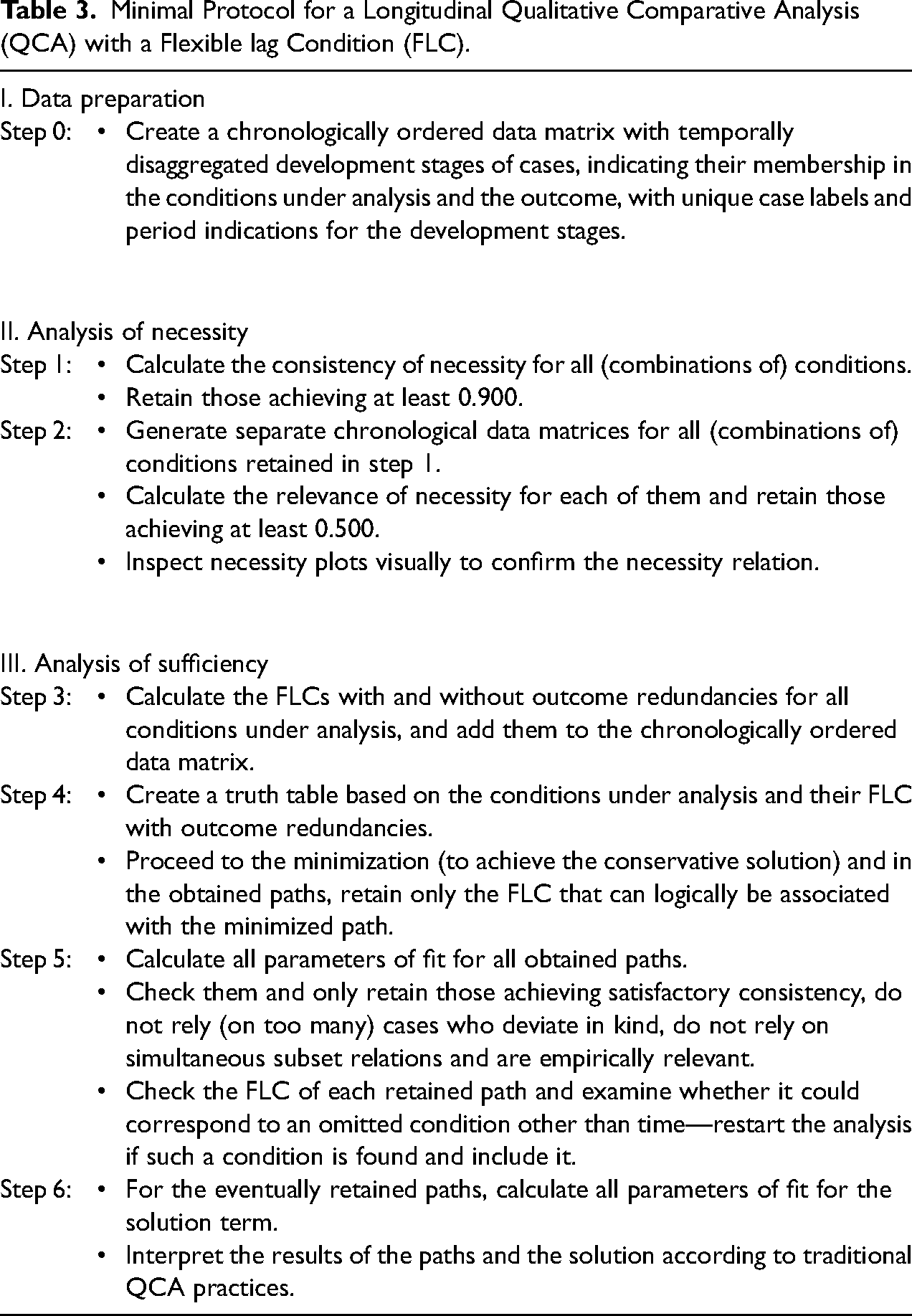
From the description of these first two steps, it follows that the analysis of necessity does not involve any FLC. It is not entirely “time blind”, though, insofar as the chronological order of the conditions based on CBIs remains important for the definition of what is considered as a different development stage of a case and is therefore taken into consideration as a distinct unit in the analysis of necessity. Beside from relying on temporally disaggregated cases, however, the analysis of necessity does not dig further into the importance of time for the occurrence of the outcome.

Step 3. The analysis of necessity is followed by the analysis of sufficiency. To prepare it, the FLCs with and without outcome redundancies need to be calculated for all conditions under analysis and added to the data matrix. The function FLC.df can be used for that (see the online Appendix A.1.3).

Step 4. I have shown above that in a longitudinal QCA without FLC, combinations of conditions can appear to be not sufficient for the outcome because of either time insensitive or empirically redundant contradictions. In a longitudinal QCA, one can thus not carry out the traditional truth table minimization and then calculate the FLCs for all retained paths because some paths would not be retained in the absence of an FLC in the first place. Instead, one needs FLCs to be calculated for each possible combination of conditions and then to be integrated in the minimization analysis. Furthermore, in the logical minimization, the calculated FLCs need to be combined only with the conditions they have been calculated for. For the conservative solution, this can be checked manually. For the intermediate and most parsimonious solutions, however, this requires an adapted truth table algorithm which, in light of the potentially very high number of possible combinations in a QCA,⁵ and the thus equally high number of required FLCs, I am unable to provide. The same logic applies and my proposal should be clear enough, however, for a set-theoretic programmer to take up on this.

To achieve the conservative solution, one can carry out the traditional conservative QCA minimization using a truth table that has been created based on both the conditions under analysis and their FLCs (with outcome redundancies—as argued above; their names can be obtained with function FLC.names, see the online Appendix A.1.4). In the end, however, the retained paths should only be associated with their FLC. If an obtained path features several FLCs, the non-tenable ones should be dropped because they are logically not relevant for the conjunction and mathematically a subset with identical parameters of fit. This can be achieved with the function FLC.minimize (see the online Appendix A.1.5).

Step 5. Before we can conclude that the obtained paths are sufficient for the outcome, several additional inspections need to be conducted. First, the sufficiency of each path should be judged based on the four criteria suggested by Oana, Schneider and Thomann (2021:90–101): (i) high enough consistency (judged in relation to the truth table, with scores between 0.750 and 0.800 being the acceptable minimum), (ii) avoiding cases whose consistency deviates in kind, (iii) excluding simultaneous subset relations when analyzing fuzzy sets by only retaining paths with a proportional reduction in inconsistency (PRI) of at least 0.5, and (iv) assessing the empirical relevance in terms of coverage. The consistency, PRI, coverage, and average lag duration can be calculated with the function AoS.path for any specified path (see the online Appendix A.1.6). As argued above, these calculations should take into consideration the FLC without outcome redundancies to return correct parameters of fit.

Second, beyond these regular QCA precautions, the FLC of each retained path needs to be checked as to whether it could correspond to an omitted condition other than time. If this is the case, restart the analysis with the new condition. As a standard of good practice, the full dataset and FLC distributions should be made available so this same verification can also be done by reviewers and readers. Throughout these inspections, the Show.Path.Cases function (see the online Appendix A.1.7) can be used to display the cases supporting, contradicting, and left uncovered by each path.

Step 6. All paths that satisfy these inspections can be considered part of the final solution formula(s). Its parameters can be calculated with the function AoS.sol (see the online Appendix A.1.8). In my theoretical example, whose results are summarized in Table 4, the solution term for the presence of the outcome is A*B + A*C. A is a necessary condition for the presence of the outcome with perfect consistency and satisfactory relevance. For A*B, it takes on average of 2.5 years to lead to the outcome. A*C, in turn, take on average of 7.7 years to lead to the outcome. While the former path is perfectly consistent and covers 50 percent of cases’ development stages in which the outcome is present, the later path is consistent with 75 percent of cases’ development stages and covers 75 percent of those in which the outcome is present. The confirming cases for A*B are Case 1 (1951–1955; 1956–1964) and Case 3 (1986–1989; 1990–1993). A*C are confirmed by Case 2 (1973–1977; 1978–1982), Case 3 (1986–1989; 1990–1993), and Case 4 (1952–1952), but contradicted by Case 5 (1964–1970). Case 3 (1986–1989; 1990–1993) is thus covered by both paths. Note that the second periods mentioned in parentheses are outcome redundancies and were not taken into consideration for the calculation of the parameters of fit. The entire solution is consistent with 80 percent of cases’ development stages and covers all in which the outcome is present. For the interpretation in a real application, I would encourage to dedicate further attention to the cases that support and contradict each (or multiple) path(s), as well as to those covered by none.

Table 4.

LQCA Results of the Intermediate Solution for the Theoretical Example.

Conditions		Sufficiency		Nec.
Conditions		(1)	(2)
A		⬤	⬤	⬤
B		⬤
C			⬤
D
Temporal lag (years)	Mean	2.500	7.667	-
	St. dev.	3.536	6.658	-
Consistency		1.000	0.750	1.000
PRI		1.000	0.750	-
Raw coverage		0.500	0.750	0.500
Unique coverage		0.250	0.500	-
Relevance of necessity		-	-	0.500
Solution consistency		0.800
PRI		0.800
Solution coverage		1.000
Units of observation (outcome = 1)		18 (4 \| 7)

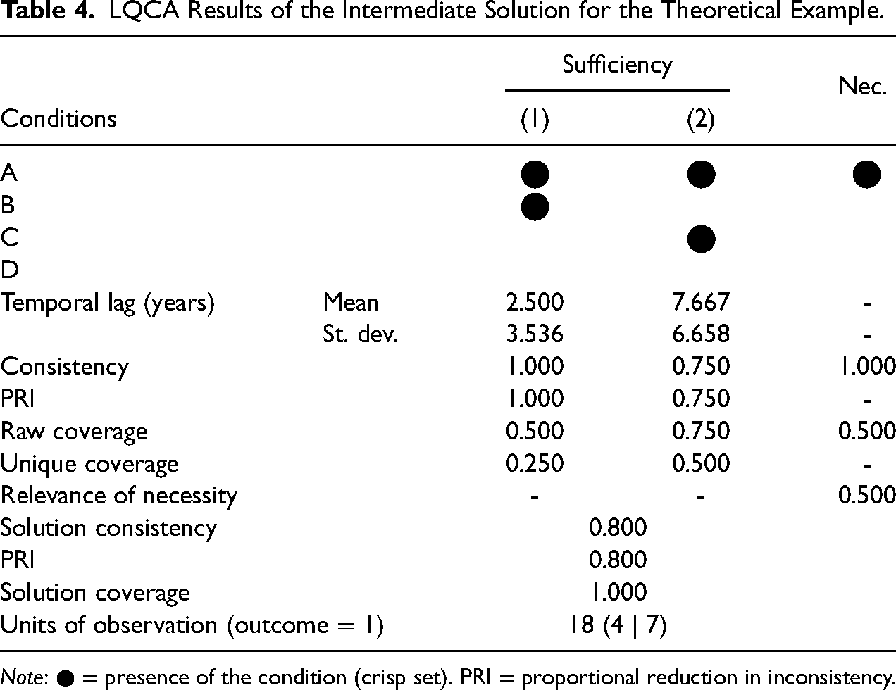
Note: ● = presence of the condition (crisp set). PRI = proportional reduction in inconsistency.

Three elements should be retained from the preceding illustration. First, the method proves successful in meaningfully resolving longitudinal research problems with a systematic set-theoretic comparison. Second, the FLC is not only useful for overcoming time-insensitive and empirically redundant contradictions, as well as outcome redundancies, but also provides interesting complementary information on the time it takes for (a combination of) conditions to translate into the outcome. Third, despite its suitability for large-n analyses, the method remains case-oriented and allows for in-depth qualitative inquiries.

Extension to Fuzzy set and Multi-Value QCA

In the previous sections, the rationale and procedure of a longitudinal QCA with FLC has been explained and illustrated based on crisp set examples. The same logic, however, could be extended quite naturally to fuzzy set and multi-value QCA, which would be a welcomed further development of the FLC approach as set out in this article. Despite the similar logic, a few particularities deserve mentioning.

For longitudinal fuzzy set QCA with an FLC, I would suggest to disaggregate cases each time a condition or the outcome change not only in kind but also in degree. As indicated previously, even if a change in degree does not alter the overall presence or absence of a condition, it consists of a new empirical reality and leads to different parameters of fit that should be taken into consideration.⁶

For longitudinal multi-value QCA with an FLC, cases should be disaggregated each time there is a (multi-value) change in a condition or the outcome. Since all changes are in-kind changes, the minimization and consistency calculations would work like for crisp sets—except that we take into consideration the multi-values. The FLC should be calculated by taking into consideration each change in the conditions and remains a crisp set itself.

Potential Pitfalls and How to Address Them

Despite the positive appraisal above, the procedure for carrying out longitudinal QCA with a FLC I suggest can be subject to three pitfalls that need to be signaled. First, there is a risk for the FLC to hide a condition that has been omitted in the analysis. To avoid this, the distribution of the FLC needs to be checked carefully for each path. Thereby, one needs to reflect if it could correspond to a factor that is not taken into consideration by the analysis. Generally speaking, the longer the average lag of a path, the higher is the probability it is underspecified and that an important condition has been omitted. One should not confuse the average length of an FLC with the omission of a condition though. It is a possible symptom but never the cause because it is calculated post hoc, after the FLC has been determined. What constitutes an acceptable average lag depends on the topic of the research and should be justified in light of the temporal dynamics that come with it. As a standard of good practice, researchers should publish the distribution of their chronologically ordered dataset and of the FLCs for each path found relevant in analysis.

Second, longitudinal case disaggregation comprises a risk for producing skewed outcomes. In longitudinal observations, it can indeed take some time (and several intervals) before an outcome occurs. This is even more true for CBIs because cases are disaggregated temporally each time cases’ membership in a condition or the outcome change. When changes in the conditions are more frequent than changes in the outcome, which is likely—certainly with an increasing number of conditions—the number of negative cases will exceed the number of positive cases. The problem of such a skew is that high levels of consistency can easily be achieved by many conditions when explaining the positively skewed absence of the outcome. If this is the case, I would recommend to either not carry out or interpret very cautiously the analysis of when the outcome is absent. Should one decide not to carry out the analysis, it needs to be emphasized that this does not exempt the QCA from its asymmetrical causality property, i.e., that the absence of the conditions leading to the presence of the outcome can still not be assumed to explain the absence of the outcome.

Third, because the integration of the FLCs in the minimization process requires a modified truth table algorithm, the procedure developed in this article can achieve the conservative solution, but not the intermediate and most parsimonious one. Future developments rendering the latter possible in the form of an algorithm capable to integrate FLCs for all possible combinations in the truth table minimization would be strong contributions to further refining the approach.

Finally, some attention should be dedicated to the choice of cases’ end point. It is not a pitfall strictu sensu of this procedure because when to observe cases is an issue in all case-based research—whether accounting for temporal variation or not. However, the present procedure comes with some particularities in this respect that should be kept in mind. The FLC works indeed well with analyses in which the occurrence of the outcome closes the development process of a case (i.e., the outcome occurs in the last temporally disaggregated development stage of a case). For analyses where an outcome can occur multiple times in the development process of a case, one can obtain contradictory configurations because the period of observation ended without the outcome occurred, although all conditions that previously led to the outcome are united. If this happens, one needs to consider carefully where to place the end of the observation, i.e., to reflect until when one thinks a case can still evolve. This “possibility of evolution” is indeed a precondition for a meaningful longitudinal analysis. Should one extend the period of observation beyond the last occurring outcome, it should be signaled if future evolutions are possible or if the case can be considered “closed”. If evolutions are still possible, contradictions observed at the end of the distribution are to be nuanced because the outcome might just not have occurred yet. If no further evolutions are possible, the contradictions observed at the end of the distribution are to be interpreted as such.

Conclusion

In this article on longitudinal QCA, I have shown (i) why change-based intervals (CBIs) should be preferred over fixed intervals if there is no particular epistemological justification for the latter and (ii) how a flexible lag condition (FLC) resolves two types of temporally contradictory configurations and outcome redundancies that can result from temporal case disaggregation. By doing so, my research pursues the work of recent methodological developments that aim to render QCA “time sensitive” and makes four main contributions.

First, it encourages both methodological works on longitudinal QCA and empirical applications to reflect on how cases are disaggregated temporally. While illustrated with fixed intervals, the existing calibration mechanisms suggested by Hino (2009) for time series QCA, the different consistency measurements proposed by Garcia-Castro and Ariño (2016) for panel data QCA, the trajectory QCA developed by Pagliarin and Gerrits (2020) and the tracking of configurations over time proposed by Verweij and Vis (2021) are all compatible with CBIs.

Second, the research has pointed out the possibility of two types of temporal contradictions to arise in a longitudinal QCA with temporally disaggregated cases that previous approaches had not yet spotted: “time insensitive” contradictions and “empirically redundant” contradictions. In parallel, it has identified the issue of empirically redundant outcome configurations.

Third, it has developed an approach to resolve these via an FLC that does not only offset the contradictions by grouping identical configurations and flexibly lagging the outcome, but that does also account for the average amount of time it takes for a (combination) of condition(s) to translate into the outcome. This enriches traditional longitudinal set-theoretic accounts with additional information on the required duration for a constellation to lead to the outcome.

Finally, the approach tries to bridge two worlds by providing a procedure that allows to analyze an important number of cases and conditions longitudinally, while at the same preserving a strong case-oriented approach. Since temporal contradictions are most likely with an increasing number of time points and conditions, as well as with CBIs in general, the FLC procedure is most useful for them. The fact that the interest of longitudinal analyses increases with the number of studied cases and conditions (Gerrits and Pagliarin 2021) underlines the usefulness of the methodological innovation I propose. Despite its suitability for mid-n and large-n analyses, longitudinal QCA with an FLC preserves a strong case-oriented and qualitative perspective and remains thereby loyal to QCA's original foundations (Ragin 1987, Rihoux and Lobe 2015). The procedure encourages indeed to fully unravel the dynamics of the studied phenomenon by inspecting and discussing the chronological development of confirming, contradictory and non-covered cases, as well as by inspecting and interpreting the lag condition. The trajectory-based approach of Pagliarin and Gerrits (2020) can constitute an interesting complement to the present procedure when the development stages and order of the condition changes are traced.

Taken together, this lets me hope that the approach presented in this article will facilitate the entrance of QCA to the field of longitudinal analyses and enrich existing small-n process tracings or large-n variance-based analyses with a set-theoretic account. At the same time, the endeavor of integrating time into QCA is far from being completed. I would hope this article to stimulate further reflections on the topic and refinements of the approach. Extending its illustration to multi-value and fuzzy set QCA, as well as developing an adapted minimization algorithm capable of achieving the intermediate and conservative solutions, seem most promising to me.

Supplemental Material

sj-pdf-1-smr-10.1177_00491241231156967 - Supplemental material for Longitudinal QCA: Integrating Time Through Change-Based Intervals (CBIs) and a Flexible Lag Condition (FLC)

Supplemental material, sj-pdf-1-smr-10.1177_00491241231156967 for Longitudinal QCA: Integrating Time Through Change-Based Intervals (CBIs) and a Flexible Lag Condition (FLC) by Christoph Niessen in Sociological Methods & Research

Footnotes

Acknowledgements

I would like to thank Gary Goertz, Sofia Pagliarin, Benoît Rihoux, Ioana-Elena Oana, Adrian Dusa, and Min Reuchamps for their comments and suggestions on earlier drafts or elements of this article. Furthermore, I wish to express my gratitude to the three anonymous reviewers of Sociological Methods and Research for their detailed and generous comments and suggestions.

Author's Note

The data and R-code used for the illustrative analysis of the minimal example can be found in the appendices.

Declaration of Conflicting Interests

The author declared no potential conflicts of interest with respect to the research, authorship, and/or publication of this article.

Funding

The author disclosed receipt of the following financial support for the research, authorship, and/or publication of this article: This research was originally funded by a FRESH (F6/40/5 – FC17963) grant from the Belgian Fonds de la Recherche Scientifique (F.R.S. – FNRS). In addition to my current affiliation, an important part of this research was carried out at Université de Namur, Université catholique de Louvain, and the European University Institute.

ORCID iD

Christoph Niessen

Notes

Author Biography

Christoph Niessen is an Assistant Professor of Comparative Politics at Leiden University. His research deals with substate autonomy dynamics in plurinational states, as well as with deliberative citizen participation.

References

Aversa

Paolo

Furnari

Santi

Haefliger

Stefan

. 2015. “Business Model Configurations and Performance: A Qualitative Comparative Analysis in Formula One Racing, 2005–2013.” Industrial and Corporate Change 24(3):655-76.

Boswell

Terry

Brown

Cliff

. 1999. “The Scope of General Theory: Methods for Linking Deductive and Inductive Comparative History.” Sociological Methods & Research 28(2):154-85.

Caren

Neal

Panofsky

Aaron

. 2005. “TQCA: A Technique for Adding Temporality to Qualitative Comparative Analysis.” Sociological Methods & Research 34(2):147-71.

Demin, Gregory. 2022. “Expss: Tables, Labels and Some Useful Functions from Spreadsheets and ‘SPSS’ Statistics. R Package Version 0.11-1.” https://CRAN.R-project.org/package=expss.

De Meur

Gisèle

Rihoux

Benoît

Yamasaki

Sakura

. 2009 “Addressing the Critiques of QCA.” pp. 147-65. in Configurational Comparative Methods: Qualitative Comparative Analysis (QCA) and Related Techniques, edited by Rihoux

Ragin

. Thousand Oaks: Sage.

Dowle

Matt

Srinivasan

Arun

. 2021. data.table: Extension of 'data.frame'. R Package Version 1.14.2”. (https://CRAN.R-project.org/package=data.table).

Dusa

Adrian

. 2019. QCA with R. A Comprehensive Resource. New York: Springer.

Dusa

Adrian

. 2022. “QCA: Qualitative Comparative Analysis. R Package Version 3.15”. (https://CRAN.R-project.org/package=QCA).

Fischer

Manuel

Maggetti

Martino

. 2017. “Qualitative Comparative Analysis and the Study of Policy Processes.” Journal of Comparative Policy Analysis: Research and Practice 19(4):345-61.

10.

Furnari

Santi

. 2018. “Four Approaches to Longitudinal QCA: Opportunities and Challenges.” Paper presented at the QCA Professional Development Workshop, Chicago Academy of Management (10 August).

11.

Garcia-Castro

Roberto

Ariño

Miguel A

. 2016. “A General Approach to Panel Data Set-Theoretic Research.” Journal of Advances in Management Sciences & Information Systems 2:63-76.

12.

Gerrits

Lasse

Pagliarin

Sofia

. 2021. “Social and Causal Complexity in Qualitative Comparative Analysis (QCA): strategies to Account for Emergence.” International Journal of Social Research Methodology 24(4):501–14.

13.

Goertz

Gary

. 2017. Multimethod Research, Causal Mechanisms, and Case Studies: An Integrated Approach. Princeton & Oxford: Princeton University Press.

14.

Hak

Tony

Jaspers

Ferdinand

Dul

Jan

. 2015 “The Analysis of Temporally Ordered Configurations: Challenges and Solutions.” pp. 107-27. in Configurational Theory and Methods in Organizational Research, edited by Fiss

Cambre

Marx

A. M.

. Bingley: Emerald.

15.

Harrell, Frank. 2022. “Hmisc: Harrell Miscellaneous. R Package Version 4.6-0.” https://CRAN.R-project.org/package=Hmisc.

16.

Hino

Airo

. 2009. “Time-Series QCA.” Sociological Theory and Methods 24(2):247-65.

17.

Oana

Ioana-Elena

Schneider

Carsten Q

Thomann

Eva

. 2021. Qualitative Comparative Analysis Using R: A Beginner's Guide. Cambridge: Cambridge University Press.

18.

Pagliarin

Sofia

Gerrits

Lasse

. 2020. “Trajectory-Based Qualitative Comparative Analysis: Accounting for Case-Based Time Dynamics.” Methodological Innovations 13(3): online

19.

Ragin

Charles

. 1987. The Comparative Method: Moving Beyond Qualitative and Quantitative Strategies. Berkeley: University of California Press.

20.

Ragin

Charles

. 1992 “‘Casing’ and the Process of Social Inquiry.” pp. 217-26. in What Is a Case? Exploring the Foundations of Social Inquiry, edited by Ragin

Becker

H. S.

. Cambridge & New York: Cambridge University Press.

21.

Ragin

Charles C

. 2000. Fuzzy-Set Social Science. Chicago & London: University of Chicago Press.

22.

Ragin

Charles

Strand

Sarah Ilene

. 2008. “Using Qualitative Comparative Analysis to Study Causal Order.” Sociological Methods & Research 36(4):431-41.

23.

R Core Team. 2022. “R: A Language and Environment for Statistical Computing”, Vienna: R Foundation for Statistical Computing. (https://www.R-project.org/).

24.

Rihoux

Benoît

Lobe

Bojana

. 2015. “The Case-Orientedness of Qualitative Comparative Analysis (QCA): Glass Half-Empty or Half-Full?” Teorija in Praksa 52(6):1039-245.

25.

Rihoux

Benoît

Ragin

Charles

2009. Configurational Comparative Methods: Qualitative Comparative Analysis (Qca) and Related Techniques. Thousand Oaks: Sage.

26.

Schneider

Carsten Q

. 2019. “Two-Step QCA Revisited: The Necessity of Context Conditions.” Quality & Quantity 53(3):1109-26.

27.

Schneider

Carsten Q

Wagemann

Claudius

. 2012. Set-Theoretic Methods for the Social Sciences. A Guide to Qualitative Comparative Analysis. Cambridge: Cambridge University Press.

28.

Spiess

A.-N.

2018. “qpcR: Modelling and Analysis of Real-Time PCR Data. R Package Version 1.4-1”. (https://CRAN.R-project.org/package=qpcR).

29.

Verweij

Stefan

Vis

Barbara

. 2021. “Three Strategies to Track Configurations Over Time with Qualitative Comparative Analysis.” European Political Science Review 13(1):95-111.

30.

Wickham

Hadley

. 2022. “stringr: Simple, Consistent Wrappers for Common String Operations. R Package Version 1.4.1”. (https://CRAN.R-project.org/package=stringr).

31.

Wickham

Hadley

Romain

François

Lionel

Henry

Kirill

Müller

. 2022. “dplyr: A Grammar of Ata Manipulation. R Package Version 1.0.8”. (https://CRAN.R-project.org/package=dplyr).

Supplementary Material

Please find the following supplemental material available below.

For Open Access articles published under a Creative Commons License, all supplemental material carries the same license as the article it is associated with.

For non-Open Access articles published, all supplemental material carries a non-exclusive license, and permission requests for re-use of supplemental material or any part of supplemental material shall be sent directly to the copyright owner as specified in the copyright notice associated with the article.

0.00 MB

0.10 MB