Improving Fairness in Criminal Justice Algorithmic Risk Assessments Using Optimal Transport and Conformal Prediction Sets

Abstract

In the United States and elsewhere, risk assessment algorithms are being used to help inform criminal justice decision-makers. A common intent is to forecast an offender’s “future dangerousness.” Such algorithms have been correctly criticized for potential unfairness, and there is an active cottage industry trying to make repairs. In this paper, we use counterfactual reasoning to consider the prospects for improved fairness when members of a disadvantaged class are treated by a risk algorithm as if they are members of an advantaged class. We combine a machine learning classifier trained in a novel manner with an optimal transport adjustment for the relevant joint probability distributions, which together provide a constructive response to claims of bias-in-bias-out. A key distinction is made between fairness claims that are empirically testable and fairness claims that are not. We then use confusion tables and conformal prediction sets to evaluate achieved fairness for estimated risk. Our data are a random sample of 300,000 offenders at their arraignments for a large metropolitan area in the United States during which decisions to release or detain are made. We show that substantial improvement in fairness can be achieved consistently with a Pareto improvement for legally protected classes.

Introduction

The goal of fair risk algorithms in criminal justice settings remains a high priority among algorithm developers and the users of those algorithms. The literature is large, scattered, and growing rapidly, but there seem to be three related conceptual clusters: definitions of fairness and the trade-offs that necessarily follow (Kleinberg, Mullainathan, and Raghavan 2017; Kroll et al. 2017; Corbett-Davies and Goel 2018), claims of ubiquitous unfairness (Starr 2014; Tonry 2014; Harcourt 2007; Mullainathan 2018), and a host of proposals for technical solutions (Kamiran and Calders 2012; Feldman et al. 2015; Hardt, Price, and Srebro 2016; Zafar et al. 2017; Kearns et al. 2018; Johndrow and Lum 2019; Lee, Resnick, and Barton 2019; Madras et al. 2019; Romano et al. 2019; Skeem and Lowenkamp 2020). There are also useful overviews that cut across these domains (Berk et al. 2018; Berk and Elzarka 2020; Mitchell et al. 2021).

In this paper, we examine risk assessments used in criminal justice settings and propose a novel adjustment to further algorithmic fairness. Because the outcome of interest is categorical, we concentrate on algorithmic classifiers. Unlike most other work, the methods we offer are in part a response to a political climate in which appearances can be more important than facts, and political gridlock is a common consequence. To help break the gridlock, we seek a remedy for algorithmic unfairness that is politically acceptable to stakeholders. In so doing, we take a hard look at what risk algorithms realistically can be expected to accomplish.

A recent paper by Berk and Elzarka (2020) provides a good start by proposing an unconventional way a fair algorithm could be trained. However, their approach lacks the formal structure we offer, which, in turn, solves problems that the earlier work cannot. Building on a foundation of machine learning, optimal transport (Hütter and Rigollet 2020; Si et al. 2021), and conformal prediction sets (Vovk, Gammerman, and Shafer 2005; Vovk, Nouretdinov, and Gammerman 2009), we suggest a justification for risk algorithms that treats members of a less “privileged,” legally protected class as if they were members of a more “privileged,” legally protected class. We use Black offenders and White offenders at their arraignments to illustrate our approach with the forecasting target of an arrest for a crime of violence. Many will claim that Black offenders are members of a less privileged, legally protected class and White offenders are members of a more privileged, legally protected class. Less freighted terms are “disadvantaged” and “advantaged” respectively. More will be said about the definition of “protected class” and the legal recourses available in the next section.

As a first approximation, if the performance of a risk algorithm can serve as an acceptable standard for the class of White offenders, it arguably can serve as an acceptable standard for the class of Black offenders. This helps to underscore that we propose altering only how different protected classes are treated by a risk classifier. We are not suggesting that a single risk algorithm can make fundamental changes throughout the criminal justice system; the reach of a criminal justice risk algorithm is far more modest. We also are not suggesting that the risk classifier must be state-of-the-art or even without significant defects. It must just be the customary procedure for Whites in a particular jurisdiction.

Like many who have written on algorithmic fairness, we consider fairness for legally protected classes; we focus on group fairness. Consistent with most work on fair algorithms, we take the definition of a protected class as given and contingent upon the application context (Coston et al. 2019: the “Fairness Definitions” section). As a statutory and legal matter, how groups of people come to be defined as a protected class is a complicated historical and political process often weakly tethered to first principles (Allen and Crook 2017). The issues are well beyond the scope of this paper.

Whatever the processes responsible for creating legally protected classes, there can be legitimate fairness concerns about treating Black offenders as if they are White. To some, we are proposing inequality of treatment. But here too, the issues are complex. There is no universal prescription of using race to formulate fairness remedies. On the use of race to counter discriminatory practices, Kim notes (2022: 5) that “As numerous scholars have pointed out, the law does not categorically prohibit race-consciousness.” Context matters. Moreover, we argue later that the protected class of Black offenders is made better off while the protected class of White offenders is not made worse off. We can achieve a form of Pareto improvement at the level of legally protected classes. This is quite different from the manner in which controversial interventions such as affirmative action for college admissions are often characterized. Some protected classes are said to be made better off by the admissions reforms while others are said to be made worse off (Regents of University of California v. Bakke 1978).

We also respond constructively to a longstanding ethical quandary in U.S. criminal justice (Fisher and Kadane 1983) commonly neglected in recent overviews of fairness (Baer, Gilbert, and Wells 2020; Mitchell et al. 2021). Should adjustments toward racial fairness use the treatment of White offenders as the baseline, the treatment of Black offenders as the baseline, or some compromise between the two? Although in principle, equality may be achieved using any shared baseline, the protected classes made better off and the protected classes made worse can differ dramatically. Unless an acceptable baseline for all is determined, there likely will be no agreement on how fairness is to be achieved. Moreover, when the baseline is not addressed along with adjustments toward fairness, one can arrive at fair results in which all protected classes are made equally worse off. It is difficult to imagine that stakeholders would find such a result palatable.

Whatever the baseline, a common and curious supposition is that any disparity in treatment or outcome between different protected groups is unfair and even discriminatory (Mason 2019). Gender provides an especially clear example. Men are disproportionately over-represented in prisons compared to women. But throughout recorded history, men disproportionately have committed the vast majority of violent crimes. Is the incarceration gender disparity explained solely by unfairness? For criminal justice more broadly, finding comprehensive explanations for racial disparities likewise is challenging (Hudson 1989; Yates 1997). We do not pretend to have a definitive resolution but offer instead what we hope is a politically acceptable approach.

Finally, treating Black offenders as if they are White, complicates how the appropriate risk estimands should be defined. Necessarily, counterfactuals in some form are being introduced because Black offenders cannot be White offenders, and a fair risk algorithm does not make fair all criminal justice decisions and actions that follow. We discuss these issues in the context of estimates produced by a classifier and also with confusion tables and conformal prediction sets. In so doing, we introduce counterfactual estimands to help clarify distinctions between fair risk assessment procedures and fairness in the criminal justice system more generally. The two are often conflated. A risk procedure ends with the output of a risk tool. Everything that follows, whether decisions or actions, are features of the criminal justice system beyond the risk algorithm. This will be a significant theme in the pages ahead.

In the “Conceptions of Algorithmic Fairness for Protected Classes” section, we discuss definitions of fairness in the statistics and computer science literature, commonly associated with criminal justice risk assessment, and introduce two key concepts: internal fairness and external fairness. The “Achieving A Fair Criminal Justice Risk Assessment Procedure” section summarizes the methods we use to improve fairness in criminal justice risk assessments: how a classifier should be trained, how to make comparable joint distributions of the covariates from different protected classes, and how to gauge fairness using conformal prediction sets. These methods are discussed more thoroughly and didactically in Appendices A through E. “The Data” section describes the data to be analyzed: 300,000 individuals who are arraigned shortly after an arrest and subsequently released. the “Fairness Results” section discusses the results; can post-release arrests for a crime of violence be usefully and fairly forecasted? In the “Evaluating Fairness in the Algorithmic Determinations of Risk” section, we return in depth to the empirical results shown as conformal prediction sets. The “Discussion” section suggests some possible generalizations, and the “Conclusions” section provides conclusions.

Conceptions of Algorithmic Fairness for Protected Classes

We are concerned in this paper with group fairness. Legally protected classes are the groups. Just as in formulations of group fairness, protected classes have a different conceptual status from their constituent individuals. Their legal status can differ as well.

Some Background on Legally Protected Classes

Under the U.S. Civil Rights Act of 1964, and subsequent federal anti-discrimination statutes, a “protected class” is a collection of people that can have explicit protection against discrimination, consistent with the 5th and 14th Amendments to the United States Constitution. Protected classes in anti-discrimination law are called “suspect classifications” in constitutional law. Examples of attributes that characterize protected classes are race, religion, national origin, and gender.

The protection takes the form of judicial scrutiny, which can vary in intrusiveness, but it only opens the door to an examination of the setting, the specific facts, and how well-tailored the use of class membership may be (Kim 2022). There are no foregone conclusions. From a litigation perspective, moreover, class membership is not automatic. For example, a particular black employee is not a member of a protected class until the employee formally alleges, say, disparate treatment in wages by his or her employer. The class membership persists only until the end of the legal dispute. ¹

This leads to some semantic ambiguities. For example, race is commonly called a protected class that can include several different races such as Whites, Blacks, and Asians. It is then also common to speak of particular Whites, Blacks, or Asians, as a protected class when they seek legal redress for discrimination. In context, however, there should be no confusion.

Fairness Definitions

Even for legally protected classes, there is no constitutional guidance for definitions of algorithmic fairness, in part because jurisprudence is still trying to catch up. There are no prescribed empirical methods. And, there is not even a common language to address the issues (Huq 2019; Mason 2019). Nevertheless, researchers have proposed a variety of algorithmic fairness types.

The definitions to follow arise directly from confusion tables and are easily translated into many common fairness typologies employed in risk assessment (Kleinberg, Mullainathan, and Raghavan 2017; Kroll et al. 2017; Berk et al. 2018; Berk and Elzarka 2020; Mitchell et al. 2021). Other definitions briefly are considered in due time. Anticipating our later data analyses, we use White criminal justice offenders and Black criminal justice offenders at their arraignments as illustrations of the protected classes for which fairness is sought. Fairness centers on their algorithmic forecasts of risk. Is the algorithmic output itself fair?

Prediction parity. The predictive distributions across protected classes are the same. Prediction parity can be estimated with test data by, for example, the proportions of Black offenders or White offenders forecasted to be arrested after an arraignment release. Prediction parity is sometimes called demographic parity.

Prediction parity properly is judged by the risk tool output alone, not by the decisions that follow, not by any subsequent actions or occurrences, and not by the true but unknown outcomes. An important implication is that the actual outcome class to be forecasted (e.g., an arrest) has no role in the definition of prediction parity. As a result, prediction parity has been criticized as unsatisfactory and even irrelevant (Hardt, Price, and Srebro 2016). Yet, an absence of prediction parity may be linked to “mass incarceration,” which in practice cannot easily be disregarded. Moreover, requiring the inclusion of the actual outcome class in fairness definitions leads to challenges we discuss shortly.

Classification parity. The false positive rates and false negative rates are the same across protected classes. A false positive denotes that a risk algorithm incorrectly classified a case with a negative class label as a case with a positive class label. A false negative denotes that a risk algorithm incorrectly classified a case with a positive class label as a case with a negative class label. 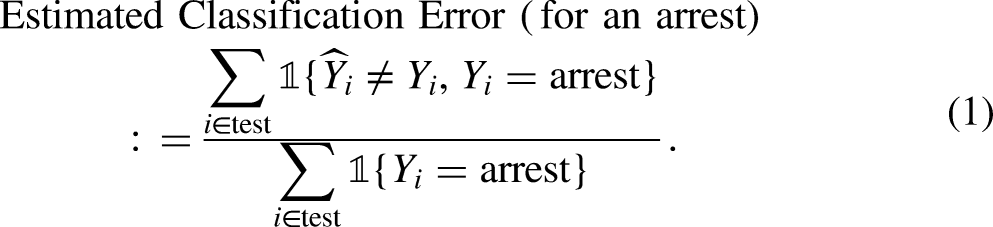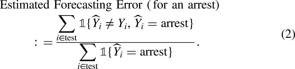² The false positive rate and a false negative rate are the respective probabilities over cases that the algorithm classifies outcomes erroneously. When there are more than two outcome classes, classification parity follows from the same reasoning, but there are no standard naming conventions.

Ideally, false positive and false negative rates are estimated with test data. Classification error for a particular outcome class, such as an arrest, is the proportion of subjects erroneously classified as not arrested among all who actually were arrested. If an arrest is the negative class, for example, one has an estimate of the false positive rate. More formally,

$$\begin{array}{cc}& \text{Estimated Classification Error (,for an arrest)}\\ & :=\frac{{\displaystyle \sum _{i\in \mathrm{test}}\mathbb{1}\{{\hat{Y}}_i\ne Y_i,Y_i=\text{arrest}\}}}{{\displaystyle \sum _{i\in \mathrm{test}}\mathbb{1}\{Y_i=\text{arrest}\}}}.\end{array}$$

(1)

$Y_i$ is the true outcome for subject $i$ in test data, and ${\hat{Y}}_i$ is the forecasted, test data outcome from the trained classifier (i.e., usually the outcome with the highest estimated probability). The classification error in (1) is an estimator for $\mathbb{P}(\hat{Y}\ne Y|Y=\text{arrest})$ . Note that one conditions on the true outcome class.

Classification error, whether through false positives or false negatives, has played a central role in fairness discussions by statisticians and computer scientists (Baer, Gilbert, and Wells 2020). However, it is often irrelevant to stakeholders, who in practice care far more about forecasting accuracy. In real forecasting settings, the actual outcome is unknown, and any subsequent decisions can be primarily informed by the forecasted outcome. Further, emphasizing classification may encourage interpretations akin to the prosecutor’s fallacy (Thompson and Schumann 1987); classification accuracy is used inappropriately to evaluate forecasting accuracy.

Forecasting accuracy parity. Each outcome class is forecasted with equal accuracy for each protected class. A forecast is incorrect if the forecasted outcome does not correspond to the actual outcome. In contrast to classification parity, one condition on the forecasted outcome not the actual outcome.

Here too, estimation should be undertaken with test data. The forecasting error for a particular outcome, such as an arrest, is the proportion of subjects erroneously forecasted to not be arrested among all subjects for whom an arrest was the forecast. Formally,

$$\begin{array}{cc}& \text{Estimated Forecasting Error (,for an arrest)}\\ & :=\frac{{\displaystyle \sum _{i\in \mathrm{test}}\mathbb{1}\{{\hat{Y}}_i\ne Y_i,{\hat{Y}}_i=\text{arrest}\}}}{{\displaystyle \sum _{i\in \mathrm{test}}\mathbb{1}\{{\hat{Y}}_i=\text{arrest}\}}}.\end{array}$$

(2)

The notation $Y_i$ and ${\hat{Y}}_i$ is the same as for classification parity. Implemented with test data, forecasting error (2) is an estimator for $\mathbb{P}(\hat{Y}\ne Y|\hat{Y}=\text{arrest})$ . In practice, only the forecasted outcomes are available to inform pending criminal justice decisions about particular individuals. This is different from algorithm training and evaluation using historical data, which typically has actual outcomes.

In some formulations, achieving forecasting accuracy parity requires that the forecasts are calibrated. For example, suppose a risk tool projects for certain offenders an arrest probability of 0.68. For calibration to be achieved, the actual arrest probability for all such offenders must also be 0.68. (Baer, Gilbert, and Wells 2020). The same reasoning applies to the estimated arrest probabilities for each outcome class. By itself, this criterion is silent on fairness, but it restricts discussion of forecasting accuracy parity to applications in which a risk tool is by this yardstick performing properly. In practice, calibration can be very difficult to attain for criminal justice risk algorithms – with good reason (Gupta, Podkopaev, and Ramdas 2020; Lee et al. 2022). This is a major theme to which we will return later.

Cost Ratio parity. The relative costs of false negatives to false positives (or the reciprocal), as defined above, are the same for each protected class. The cost ratio determines the way in which a risk assessment classifier trades false positives against false negatives. Commonly, some risk assessment errors are more costly than others, but the relative costs of those errors should be same for every protected class. The same reasoning applies when there are more than two outcome classes. ³

For reasons that become more apparent shortly, we focus primarily on prediction parity when we consider how one can construct a useful risk algorithm that forecasts arrests for crimes of violence. We aim to have the same proportions of Black and White offenders assigned to each forecasted outcome; there should be prediction parity for these two protected classes. This is a canonical risk algorithm aspiration. To succeed, however, one must overcome several formidable obstacles, some of which are not always appreciated.

Obstacles in Practice

Practice usually demands that when each kind of parity is evaluated, some form of legitimate comparability is enforced. For instance, if a risk algorithm forecasts that Black offenders are far more likely to be rearrested than White offenders, there is a prediction disparity. But in the training and test data, perhaps Black offenders tend to be younger, and the algorithm may properly recognize that younger individuals are more inclined to commit violent crimes. In this instance, the class of Black offenders and the class of Whites offenders are not similarly situated. Until this is effectively addressed, one cannot determine whether the disparity between the two protected classes is unfair.

For much of the current fairness literature, whether observational units that comprise protected classes are similarly situated is primarily a technical problem that boils down to methods that adjust for racial confounders, sometimes in a causal model. Typically overlooked is that candidate confounders possess normative as well as causal content, and both affect how confounders are selected. On the closely related notion of culpability, Horder observes (1993: 215) “…our criminal law shows itself to be the product of the shared history of cultural-moral evolution, assumptions, and conflicts that is the mark of a community of principle.” As a result, controversies over fairness often begin with stark normative disagreements about what it means to be similarly situated. For example, should an offender’s juvenile record matter in determining whether cases are similarly situated? The answer depends in part on how in jurisprudence psychosocial maturity is related to culpability (Louffler and Chalfin 2017).

Normative considerations also can create striking incongruities. Official sentencing guidelines, for example, often prescribe that defendants convicted of the same crimes and with the same criminal records should receive the same sentences. Under these specific guidelines, such defendants are similarly situated (Ostrom, Ostrom, and Kleinman 2003: chapter 1). “Extralegal” factors such as gender, race, and income are not properly included in that determination. But if “criminal records” are significantly a product of gender, race, and income, should they not be extralegal as well? The extensive literature on fairness cited earlier makes clear that there is no satisfactory answer in sight. In the pages ahead, we offer a pragmatic way forward.

There is more clarity about provable trade-offs between certain forms of parity and between parity, accuracy and transparency that are folded into discussions of fairness (Barocas, Hardt, and Narayanan 2018; Coglianese and Lehr 2019; Diana et al. 2021; Kleinberg, Mullainathan, and Raghavan 2017; Kearns and Roth 2020; Mishler and Kennedy 2021). Hard choices necessarily follow that in applications cannot be made solely for mathematical convenience. Value-driven compromises of various kinds are in practice inevitable. There does not seem to be at this point any technical resolution allowing stakeholders to have it all.

Finally, there is no empirical standard for how small disparities in parity must be for the parity to be acceptable, although most stakeholders agree that small disparities may suffice. ⁴ Interpretations of “small” will be contentious because harm depends on facts and judgments that are easily disputed. Moreover, there usually is no clear threshold at which some amount of harm becomes too much harm. Similar issues arise across a wide variety of litigation domains (Gastwirth 2000). The fairness literature has been silent on the matter, and we do not address it here. It is peripheral to our discussion of fairness, but for fair algorithms to be used effectively in practice, a binding resolution is required.

Counterfactuals: Internal and External Fairness

Despite the challenges, one has estimators for the four kinds of parity (and more) that can be employed with the usual test data. Organizing the test data separately into a confusion table for each protected class, one easily can consider the degree to which each kind of parity is achieved. When each kind of parity is examined using a combination of test data and algorithmic output, one is assessing what we call internal fairness.

Prediction parity is a very important special case. Because outcome labels are unnecessary for its definition, one legitimately can examine this form of algorithmic fairness from test data and algorithmic output alone. If the distribution of outcome forecasts is not sufficiently alike across protected classes, one properly may claim that prediction parity has been violated. ⁵

Such claims may really matter. Recall that an absence of prediction parity can be a driving force for mass incarceration. Mass incarceration usually refers to the over-representation of Blacks in the jails and prisons in the United States and is seen by some as a modern extension of slavery (Wacquant 2002). It has been a “hot button” issue for over a decade (Lynch 2011), perhaps second only to police shootings in visibility and rancor.

For classification parity, forecasting accuracy parity, and cost ratio parity, one must have the labels for the actual outcomes because those labels are built into their fairness definitions. Typically, each observation in the training and test data has such a label. Yet, we have defined internal fairness such that it depends on test data outcome labels that represent a status quo, which can include racial disparities carried forward as an algorithm is trained and fairness is assessed. For our approach to fairness that treats Black offenders as if they are White, such labels may be especially misleading. We prove in the online Appendix D that, except for prediction parity, isolating the fairness of a risk algorithm requires untestable causal assumptions that cannot be enforced in practice. These include rank preservation and strong unconfoundedness in how the criminal justice system might treat a person if he or she were of a certain race. ⁶

In short, no matter the number of observations or how the data are collected, test data outcome labels for Black offenders, such as an arrest, cannot be assumed to accurately capture the counterfactual of policing in which Blacks are treated the same as Whites. No such world is observed and represented in the data. Yet, accurate information about counterfactuals is a prerequisite for what we call external fairness. External fairness is a function for protected classes of the risk algorithm and unobserved fair counterfactuals.

Accurate information about fair counterfactual outcomes is also needed to calibrate risk algorithms properly. In particular, if a risk algorithm achieves a form of fairness by treating Black offenders as if they are White, calibration with respect to the true outcome in test data can be undermined by post-release factors that affect Blacks differently from Whites. For example, a statistical adjustment toward fairness for offenders’ prior records may weaken a substantial predictive association, caused by “overpolicing,” between longer prior records and an increased chance of a new arrest.

There are other fairness definitions in the literature for which the concerns effectively are the same. “Separation” requires that the forecasted outcome be independent of class membership, given the true outcome (Hardt, Price, and Srebro 2016). “Sufficiency” requires that the true outcome be independent of class membership, given the forecasted outcome (Baer, Gilbert, and Wells 2020). “Predictive parity” (not prediction parity) requires that the probability of the true outcome conditional on the forecasted outcome be the same when one also conditions on class membership (Chouldechova 2017). As before, the fundamental challenge is that the counterfactual outcome for Black offenders is not available in the test data.

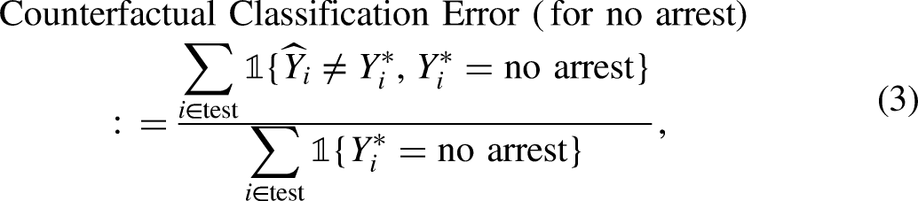
Consider, for example, counterfactual classification parity as a form of external fairness, where

$$\begin{array}{cc}& \text{Counterfactual Classification Error (,for no arrest)}\\ & :=\frac{{\displaystyle \sum _{i\in \mathrm{test}}\mathbb{1}\{{\hat{Y}}_i\ne Y_i*,Y_i*=\text{no arrest}\}}}{{\displaystyle \sum _{i\in \mathrm{test}}\mathbb{1}\{Y_i*=\text{no arrest}\}}},\end{array}$$

(3)

and $Y_i*$ in our formulation denotes the underlying counterfactual outcome for a Black offender treated upon release as a similarly situated White offender. ${\hat{Y}}_i$ is the forecast from the trained algorithm. A Black offender’s $Y_i*$ cannot be observed.

Counterfactual outcomes of this sort underscore that all criminal justice risk algorithms necessarily have a circumscribed reach. They are computational procedures that transform the input with which the algorithm is provided into information intended to help inform decisions. One can legitimately ask, therefore, if the algorithmic output by itself is fair; is the algorithm “intrinsically” fair? A criminal justice risk algorithm is not responsible for the deployment of police assets, the tactics that police employ, easy access to firearms, gang rivalries, and myriad other factors that can affect the likelihood of a post-release arrest. Outcome labels in test data incorporate these factors over which a risk algorithm has no control, and these can produce misleading assessments of classification parity, forecasting accuracy parity, and cost ratio parity. One can have an algorithm, which itself is fair despite what an analysis using test data shows. Put more strongly, stakeholders are being unrealistic to demand a fair risk algorithm to fix widespread inequities in the criminal justice system and the social world more generally. ⁷

It follows that proper evaluations of classification parity, forecasting accuracy, and cost ratio parity may be at this point largely aspirational. Within our approach to fairness and later empirical application, there is no apparent path to sound estimates of the counterfactual world in which race has no role in arrests after an arraignment release such that Black offenders are treated the same as similarly situated, White offenders. One might choose instead to assume that race is unrelated to the many causes of an arrest, but that would be contrary to the overwhelming weight of evidence (Muller 2021; Robert Wood Johnson Foundation 2017; Rucker and Rocheson 2021). ⁸

Other forms of counterfactual reasoning have been proposed for the consideration of fairness. For example, Misher and Kennedy (2021; the “Fairness Definitions” section) note the potential importance of a race counterfactual somewhat like ours. (i.e., What would happen if an individual’s race were different?) Nabi, Malinsky, and Shpitser (2019) offer a directed acyclic graph (DAG) formulation for fair policies steeped in counterfactuals but requiring assumptions that would be difficult to defend in criminal justice settings. Kusner et al. (2017) provide a DAG framework for examining racial counterfactuals, but it too requires rather daunting assumptions of the sort relied upon in many social science applications (Freedman 2012). Imai and Jaing (2021) use counterfactual reasoning to define the concept of “principal fairness,” which if achieved, subsumes many of the most common kinds of fairness, but requires conditioning on all relevant confounders. The formulation proposed by De Lara et al. (2021), using counterfactual thinking, optimal transport, and related tools, is strongly connected to some aspects of our formulation but makes no distinction between disparities and unfairness such that, for example, there can be “bona fide occupational qualifications” under Title VII of the U.S. Civil Rights Act of 1964, Section 625. ⁹

These interesting papers (see also Mitchell et al. 2021) apply a rich variety of counterfactual ideas to fairness. However, they do not consider many of the foundational fairness concerns raised earlier, such as the need for a fairness baseline or the meaning of “similarly situated.” As a result, they currently are some distance from applications in real settings where risk algorithms can directly affect people’s lives. They also differ substantially in method and focus from our approach, to which we turn shortly.

Finally, there is a small but powerful literature on fairness for individuals. An early insight is that a fair algorithm at the level of protected classes can be unfair at the level of protected class members. Similarly situated individuals are not necessarily treated similarly (Dwork et al. 2012). A solution requires a scale of individual fairness having acceptable mathematical and normative properties. There is apparently no such scale for which there is a meaningful consensus, although some progress has been made (Mukherjee et al. 2020). Perhaps more fundamentally, it may be that class fairness and individual fairness are inherently incompatible (Binns 2020; Zemel et al. 2013). Under these circumstances, individual fairness, although an important concern, is not considered further. There currently are far too many unresolved issues that are beyond the scope of this paper.

Achieving A Fair Criminal Justice Risk Assessment Procedure

When a criminal justice risk algorithm is trained, the data consist of two parts. There are predictors, and there are outcome labels. The former are used to fit the latter. Both can be responsible if racial disparities are carried forward when a risk algorithm is trained.

Even when race is not included among the predictors, it is widely understood that all other predictors can have racial content (Berk 2009). For example, the number of prior arrests may be on average greater for Blacks offenders than for White offenders. Black offenders may also tend to be younger and have been first arrested at an earlier age. Customary outcome categories used in training algorithmic risk assessments represent adverse contacts with the criminal justice system, such as arrests or convictions. Associations with race are typical here as well.

There are lively, ongoing discussions about why such racial associations exist (Allen and Crook 2017; Alpert, Dunham, and Smith 2007; Harcourt 2007; Gelman, Fagan, and Kiss 2012; Grogger and Ridgeway 2012; Starr 2014; Tonry 2014; Stewart et al. 2020). Some explanations rest on charges of racial animus in the criminal justice system, some focus on criminal justice practices properly motivated but with untoward effects, some take a step back to larger inequalities in society that propagate crime, and some frame the discussion as but one instance of widespread measurement error caused by sloppy data collection and processing.

It is likely that some mix from each perspective is relevant, but there is no credible integration yet available. Therefore, as a scientific matter, we take no position in this paper on explanations for the role of race, although a range of associations are empirically demonstrable. Rather, we more simply build on professed differences in privilege consistent with extensive research (Rothenberg 2015; Rocque 2011; Van Cleve and Mayes 2015; Leonard 2017; Wallis 2017; Bhopal 2018; Edwards, Lee, and Esposito 2019; Jackson 2019; GBD 2019 Police Violence Subnational Collaborators 2021). From a pragmatic point of view, we are responding as well to common suppositions and frequent stakeholder claims.

We do not require, more generally, that all relevant covariates are included in a criminal justice risk algorithm. An effective forecasting algorithm need not be a causal model for which potential misspecification is always an issue. Indeed, some have argued that an algorithm is not a generative model to begin with (Breiman 2001; Berk, Kuchibhotla, and Tchetgen Tchetgen 2022). Although it may at first seem shamelessly expedient, we adopt the practical goals solely of more fair, accurate, circumscribed assessments of risk than current practice. Calibration is no longer in the mix. Nor is specification error; with no modeling aspirations, misspecification is not even defined. Empirical evidence evaluating this approach is provided later.

We proceed in three steps: (1) training the risk algorithm in a novel manner, (2) transporting the predictor distribution from the less privileged class to the more privileged class, and (3) constructing conformal prediction sets to serve as risk forecasts. Each step is briefly summarized next. More details come later.

Training The Classifier

We train a machine learning classifier only on White offenders; both the predictors and the outcome are taken solely from Whites. Training on White offenders has several important consequences for our approach to fairness. ¹⁰

No distinctions between White and Black offenders, invidious or otherwise, can be made as the classifier is trained because the algorithm has information exclusively on White offenders; race is a constant. This is not to say that there are no important empirical differences between Black and White offenders. Indeed, there are likely to be important differences that we address shortly with optimal transport.

Because the training is undertaken solely with data from Whites, claims of measurement error in the training and test data caused by racial animus or structural racism can be difficult to sustain. For example, a White individual’s prior record or post-release chances of arrests are unlikely to be inflated by “overpolicing.” Many would argue that a substantial portion of the training data would be tainted by such factors if Black offenders were included.

Training on White offenders provides an algorithmic risk baseline and a potential fairness target for Blacks. Insofar as White offenders are relatively advantaged compared to Black offenders, White algorithmic performance might be seen as desirable for Black offenders; it becomes a target for fairness. One has a prospective answer to the question “fair compared to what?” The answer is fair compared to how White offenders are treated. No larger fairness claims are made.

White offenders are classified no differently than they would be ordinarily if there were no Black offenders at all; for White offenders, our fairness approach entails no intervention.

In short, by training only on Whites, we address many of the fairness complications discussed earlier.

Subsequently, when risk forecasts are sought from unlabeled data for White offenders, one can proceed as usual by obtaining predictions from the trained classifier. Nothing changes from usual practice. However, risk forecasts for unlabeled Black offenders obtained using the White-trained algorithm still can produce racial disparities because Black offenders can have more problematic predictor distributions, whatever their cause. Many Black offenders then might well be treated by the White-trained classifier as particularly risky White offenders, leading to less favorable forecasted outcomes. Another step toward fairness is needed.

Transporting Observations Across Protected Groups

A second adjustment is required to make comparable the joint distribution of predictors for Black offenders and the joint distribution of predictors for White offenders. We use a Kantorovich form of optimal transport (Hütter and Rigollet 2020; Manole et al. 2021; Pooladian and Niles-Weed 2021) to that end. Optimal transport maps the feature vector from the black population to a feature vector from the white population. To take a toy example, an arrested Black offender 18 years of age, with 3 prior robbery arrests and a first arrest at age 14, might be given predictor values from an arrested White offender who was 20 years age with 1 prior robbery arrest, and a first arrest at age 16.

Used in this manner, optimal transport is not a model. Nor is it an exercise in matching. For the toy example, both covariate point masses are within the same ${\mathbb{R}}^4$ . Each observation in the joint covariate distribution for Black offenders is “transported” to the closest observation in the joint covariate distribution for the White offenders, where closeness is defined by the squared Wasserstein distance (much like squared Euclidean distance), and the marginal distributions for Black and White offenders are fixed. One has a linear programming formulation in which the sum of the squared Wasserstein distances is made as small as possible subject to the two sets of marginal constraints (Peyré and Cuturi 2019: chapter 3; Hütter and Rigollet (2020: section 6.1)). Ideally, the joint covariate distribution for Black offenders becomes virtually identical to the joint covariate distribution for White offenders, which when used with the White-trained classifier, determines what we mean by treating Black offenders as if they were White offenders when recidivism risks are estimated.

There is one more technical detail. The transported joint predictor distribution for Black offenders is then smoothed with a form of nonparametric regression so that it can properly be used to transport predictors from new, unlabeled cases for which forecasts are needed. Details and pseudocode are provided in the online Appendix B. Further discussion can also be found later in the application.

Forecasting for Individual Cases

The practical task for a criminal justice risk assessment is to forecast one or more behavioral phenomena. By training a classifier only on White offender data and evaluating fairness separately using White test data and transported Black test data, one can as usual compare the aggregate performance of a risk assessment tool across protected classes using conventional confusion tables. There also can be forecasts for individuals that minimize Bayes risk. But we emphasize again that fairness for legally protected classes is being sought. The enterprise remains group fairness. We have nothing to say about whether a given offender is being treated fairly.

Arguably, a more defensible forecasting approach rests on conformal prediction sets (Vovk, Gammerman, and Shafer 2005; Vovk, Nouretdinov, and Gammerman 2009; Shafer and Vovk 2008; Romano et al. 2019; Kuchibhotla and Berk 2021). For a categorical response variable, a prediction set can include one or more future outcome classes with an associated probability that the prediction set includes the true outcome. For example, a prediction set could be a forecasted arrest for a violent crime that is provably true with a probability of, say, 0.90. Or the prediction set might be a forecast of an arrest for a violent crime or an arrest for a non-violent crime that is provably true with a probability of, say, 0.95. Prediction sets have some of the look and feel of confidence intervals, but the object being estimated is not a parameter of some distribution but a future outcome class. Conformal prediction sets have valid coverage in finite samples of realizations for the population from which the exchangeable data originated. The online Appendix C provides more complete treatment and pseudocode for the form of conformal inference we employ. There is further discussion in the application.

A Diagrammatic Summary of Our Risk Algorithm

Procedural details are provided in two diagrams with brief explanations for our entire risk algorithm from the training of a classifier to the use of optimal transport, to the output of a conformal prediction set. Figure 1 addresses how the fair algorithm was constructed. Figure 2 addresses fair forecasting. Both figures are further unpacked in the appendices. In addition, the data analysis to come provides a grounded methodological discussion.

Figure 1.

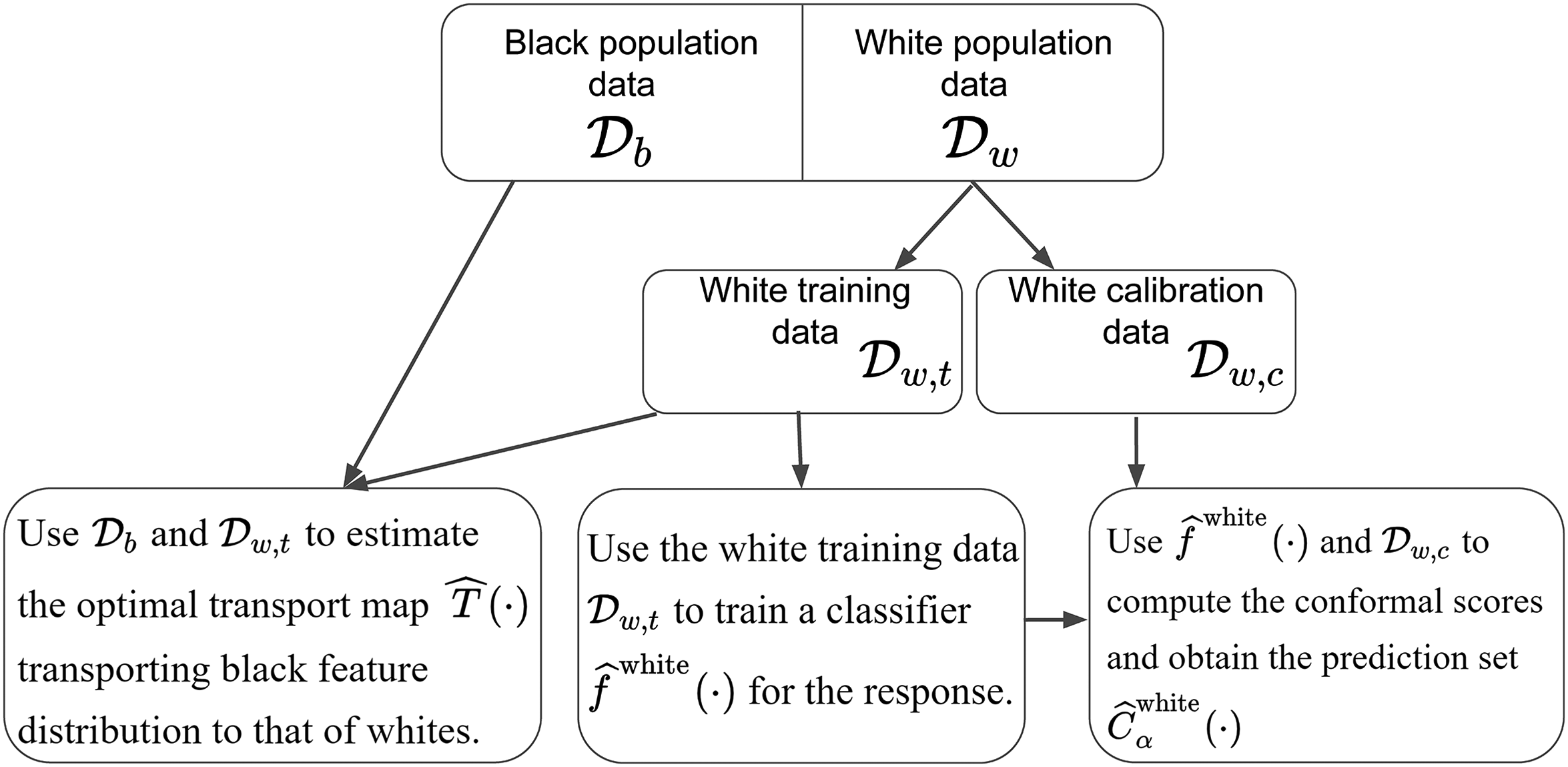
Flowchart for the training part of our “fair” risk algorithm. The function ${\hat{f}}^{\mathtt{w}\mathtt{h}\mathtt{i}\mathtt{t}\mathtt{e}}(\cdot )$ denotes the output vector of probabilities for each outcome obtained from a classifier fit on the White training data. The map $\hat{T}(\cdot )$ denotes the estimate of the optimal transport map; see the online Appendix B (and Algorithm 2) for details. The set ${\hat{C}}_{\alpha }^{\mathtt{w}\mathtt{h}\mathtt{i}\mathtt{t}\mathtt{e}}(\cdot )$ is the conformal prediction set obtained using ${\hat{f}}^{\mathtt{w}\mathtt{h}\mathtt{i}\mathtt{t}\mathtt{e}}(\cdot )$ and the White calibration data; see the online Appendix C (and Algorithm 3) for details.

Figure 2.

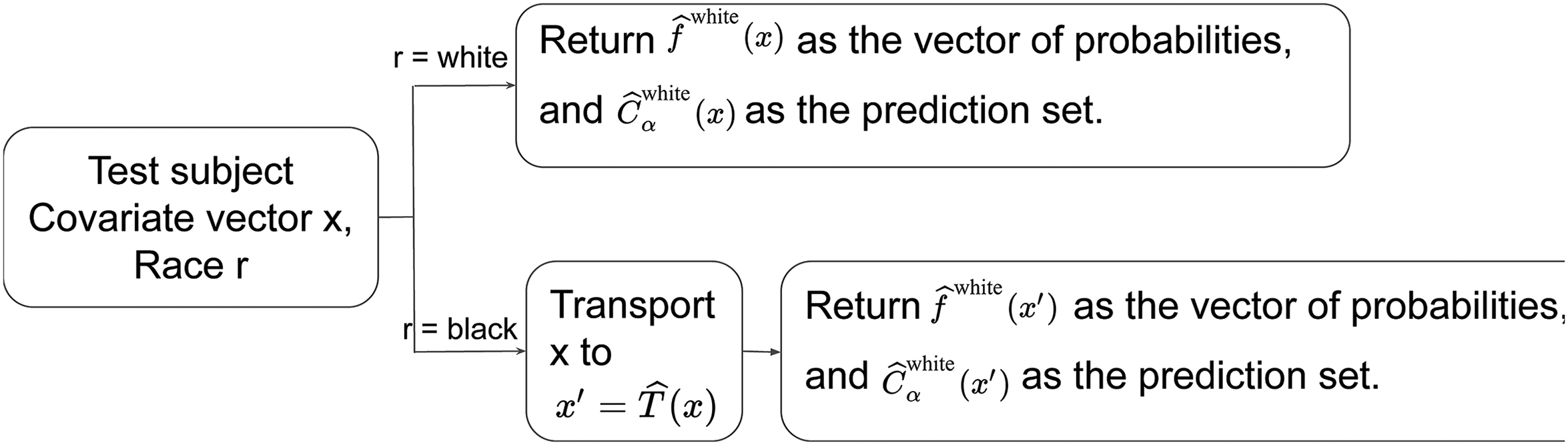
Flowchart for producing fair conformal prediction sets. The function ${\hat{f}}^{\mathtt{w}\mathtt{h}\mathtt{i}\mathtt{t}\mathtt{e}}(\cdot )$ denotes the output vector of probabilities for each outcome obtained from a classifier fit on the first split White training data. The map $\hat{T}(\cdot )$ denotes the estimate of the optimal transport map obtained from the first split training data for Whites and Blacks; see the online Appendix B for details. The set ${\hat{C}}_{\alpha }^{\mathtt{w}\mathtt{h}\mathtt{i}\mathtt{t}\mathtt{e}}(\cdot )$ is the conformal prediction set obtained using ${\hat{f}}^{\mathtt{w}\mathtt{h}\mathtt{i}\mathtt{t}\mathtt{e}}(\cdot )$ and second split white training data.

In theory, we achieve our overall goal of constructing a fair algorithmic risk tool. But in practice, there are two challenges. First, our procedures must be implemented with data having many potentially important offenders features discarded, usually for legal or political objections. Second, as a formal matter, external fairness parities cannot be evaluated from test data without very strong assumptions discussed in the online Appendix D. Recall that the required counterfactual outcome of a fair arrest-generating process is unobservable for Black offenders in existing criminal justice datasets.

A Pareto Improvement for Protected Groups

Our procedures to improve fairness arguably have a more general justification. Specifically, we claim that at the level of legally protected classes, there is a Pareto improvement. Consistent with our focus on group fairness, no formal claims are made about the consequences for individuals. But in practice, Blacks may be made better off and Whites may not be made worse off on average.

We are provisionally proceeding as if White offenders at arraignment are members of an advantaged class compared to Black offenders at arraignment. There is no claim that all individual White offenders are privileged compared to all individual Black offenders. The issues can subtle, as legal scholars have emphasized (Hellman 2020: 449–552).

By training only on White offenders and transporting the Black covariate distribution to the White covariate distribution, the presence of Black offenders has absolutely no impact on risk assessments for Whites. Nothing changesbv and the class of Whites is not made worse off. But the risk algorithm treats all Black offenders as if they are White. If the class of Whites is really advantaged at arraignment, the class of Black offenders can be made better off, or at least are not made worse off. In principle, this is a Pareto improvement for legally protected classes with respect to the performance of the risk algorithm itself. We will bring data to bear later.

Consider the Civil Rights Act of 1964 as amended in 1972 to prohibit sex discrimination in educational institutions receiving federal financial assistance (i.e., “Title IX”). The landscape of college sports changed dramatically because women could expect to have their own intercollegiate sports teams. As a class, women benefited, even if the direct benefits were conferred largely on the small fraction of all female students who became varsity athletes. If athletic department budgets were increased sufficiently, a Pareto improvement was possible, determined jointly by the class of men and the class of women.

The Data

We analyze a random sample of 300,000 offenders at their arraignment from a particular urban jurisdiction in the United States. ¹¹ Because of the random sampling, the data can be treated as IID and, therefore, exchangeable. Even without random sampling, one might well be able to make an IID case because the vast majority of offenders at their arraignment are realized independently of one another.

Among those being considered for release at their arraignment, one outcome class (coded “1”) to be forecasted is whether the offender will be arrested after release for a crime of violence. An absence of such an arrest (coded “0”) is the alternative outcome class to be forecasted. Violent crimes usually are of particular concern. ¹²

The follow-up time is 21 months after release. For reasons related to the ways in which competing risks were defined, 21 months was chosen as the midpoint between 18 months and 24 months. For the analysis to follow, the details are unimportant.

Candidate predictors were the usual variables routinely available in large jurisdictions. Many were extracted from adult rap sheets and analogous juvenile records. Biographical variables included race, age, gender, residential zip code, employment information, and marital status. There were overall 70 potential predictors.

In response to potential stakeholder concerns about “bias,” we excluded from the classifier training race, zip code, marital status, employment history, juvenile record, and arrests for misdemeanors and other minor offenses. Race was excluded from the training for obvious reasons. Zip code was excluded because, given residential patterns, it could be a close proxy for race. “Close” was not clearly defined, but if offenders’ zip codes were known, one usually could be quite sure about their race. No other potential predictors were seen by stakeholders as close proxies for race. ¹³ Employment history and marital status were eliminated because there were objections to using “life style” measures. Juvenile records was discarded because poor judgment and impulsiveness, often characteristics of young adults, are not necessarily indicators of long-term criminal activity. Minor crimes and misdemeanors were dropped because many stakeholders believed that arrests for such crimes could be substantially influenced by police discretion, perhaps motivated by racial animus.

The truth underlying such concerns is not definitively known, but insofar as the discarded predictors were associated with any included predictors, potential biases remain (Berk 2009). These decisions underscore our earlier point that there are legitimate disagreements over what features of individuals should determine when a similarly situated comparison has been properly undertaken. They also highlight the trade-offs to be made when a suspect predictor also is an effective predictor.

In the end, the majority of the predictors were the number of prior arrests separately for a wide variety of serious crimes, and the number of counts for various charges at the arraignment. Other included predictors were whether an individual was currently on probation or parole, age, gender, the age of a first charge as an adult, and whether there were earlier arrests in the same year as the current (arraignment) arrest. For the analyses to follow, there were 21 predictors. ¹⁴

The 300,000 cases were randomly split into training data for White offenders, training data for Black offenders, test data for White offenders, and test data for Black offenders. Half the dataset was used as training data ( $n=150,000$ ) and half the dataset was used as test data ( $n=150,000$ ). Sizes of the racial splits of the training and test data were simply determined by the numbers of Black offenders and White offenders available in the data. Each racial split had at least 40,000 observations.

Fairness Results

We began by training a stochastic gradient boosting algorithm (Friedman 2001) on White offenders only using the procedure gbm from the library gbm in the scripting language R. For illustrative purposes and consistent with many stakeholder priorities, the target cost ratio was set at 8 to 1 (Berk 2018). Failing to correctly classify an offender who after release is arrested for a crime of violence was taken to be 8 times worse than failing to correctly classify an offender who after release is not arrested for such a crime. We were able to approximate the target cost ratio reasonably well in empirical confusion tables by weighting more heavily training cases in which there was an arrest for a crime of violence. This, in effect, changes the prior distribution of the outcome variable. ¹⁵

All tuning defaults worked satisfactorily except that we chose to construct somewhat more complex fitted values than the defaults allowed. We used greater interaction depth to better approximate interpolating classifiers Wyner et al. (2015). Even after weighting, we were trying to fit relatively rare outcomes. We needed an ensemble of regression trees each with many recursive partitions of the data.

The results were essentially the same when the defaults were changed by modest amounts. The number of iterations (i.e. regression trees) was determined empirically when, for a binomial loss, the reductions in the test data effectively ceased. ¹⁶

Algorithmic Performance Results for White Offenders

Algorithmic risk assessments can be especially challenging when the marginal distribution of the outcome is highly unbalanced. For binary outcomes, this means that if criminal justice decision-makers always forecast the most common outcome class, they will be correct the vast majority of the time. It is difficult for an algorithm to forecast more accurately. Because post-arraignment arrests for a crime of violence are well-known to be relatively rare, we were faced with the same challenge that, nevertheless, provided an instructive test bed for examining fairness.

To set the stage, Table 1 is the confusion table for White offenders using the risk algorithm trained on Whites and test data for Whites. ¹⁷ Perhaps the main message is that if arraignment releases were precluded solely by the risk algorithm when arrests for a violent crime were forecasted, more violent crimes might be prevented.

Table 1.

Test Data Confusion Table for White Offenders Using the White-Trained Algorithm (28% Predicted to Fail, 7.5% Actually Fail).

Actual Outcome	No Violence Predicted	Violence Predicted	Classification Error
No Violence	31630 (true positives)	11246 (false positives)	0.26
Violence	1527 (false negatives)	1975 (true negatives)	0.47
Forecasting Error	0.05	0.85

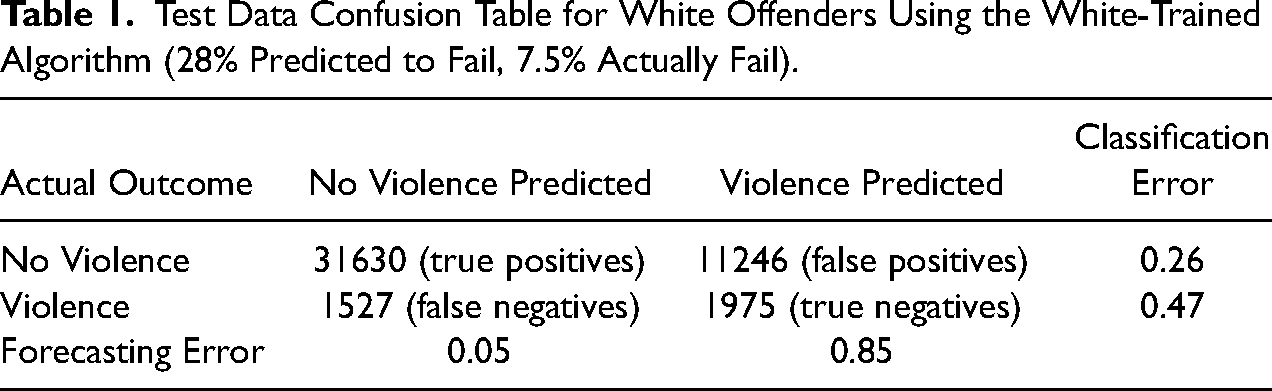
Here is the reasoning. From the outcome, marginal distribution of an arrest for a crime of violence, minimizing Bayes loss always counsels forecasting no such arrest after an arraignment release. That forecast would be wrong for 7.5% of the White offenders. From the left column in Table 1, when the algorithm forecasts no arrest for a violent crime after an arraignment, the forecast is wrong for 5% of the White offenders. If from the marginal distribution one always forecasted an arrest for a crime of violence, the forecast would be wrong for 92.5% of the White offenders. From the right column in Table 1, the algorithm is mistaken for 85% of the white offenders. These are modest improvements in percentage units, but given the large number of White offenders, over 2000 of violent crimes might be averted if the risk algorithm determined the arraignment release decision rather than the presiding magistrate with no algorithmic input. By this standard, the risk algorithm performs better.

Yet, forecasting accuracy is shaped substantially by the cost ratio. Because the target cost ratio treats false negatives as 8 times more costly than false positives, predictions of violence in Table 1 are dominated by false positives. This follows directly and necessarily from the imposed trade-offs. Releasing violent offenders is seen to be so costly that even a hint of future violence is taken seriously. But then, many mistakes are made when an arrest for a crime of violence is forecasted. In trade, when the algorithm forecasts no arrest for a violent crime, it is rarely wrong; there are relatively few false negatives. This too follows from the target cost ratio. If even a hint of violence is taken seriously, those for whom there is no such hint are likely to be very low-risk releases. In short, with different target cost ratios, the balance of false positives to false negatives would change, perhaps dramatically, which means that forecasting accuracy would change as well. ¹⁸

The aversion to false negatives contributes to a projection that 28% of White offenders will fail through a post-release arrest for a violent crime. In the test data, only 7.5% actually fail in this manner. The policy-determined trade-off between false positives and false negatives produces what some call “overprediction.” With different trade-off choices, overprediction could be made better or worse. In either case, there would likely be important concerns to reconsider.

Overprediction worries become even more pronounced if test data for Black offenders are used to forecast post-arraignment crime. When the Black test data are employed with the algorithm trained on Whites, 41% of the Black offenders are forecasted to be arrested for a crime of violence, whereas 11% actually are. The re-arrest base rate is a bit higher for Black offenders than White offenders (i.e., 11% compared to 7.5%), but the fraction projected to be arrested for a violent crime increases substantially: from 28% to 41%. As emphasized earlier, the latter disparity cannot be a product of racial differences in the algorithmic machinery. It is trained only on Whites. The likely culprit is racial disparities in the feature distribution provided to the classifier. In any case, there is clear evidence from the test data that prediction parity is not achieved solely by training the risk algorithm on White offenders.

Table 1 also provides for White offenders conventional test data performance statistics for the false positive rate, the false negative rate, forecasting accuracy for an arrest for a crime of violence, forecasting accuracy for no arrest, and the empirical cost ratio. For example, the false positive rate is 0.26 and when no arrest is forecasted, it is wrong 5% of the time. Comparisons could be made to the full confusion table for Black offenders, but the limitations of internal fairness would intrude; recall that historical test data are poorly suited for examinations of external fairness. We postpone further discussion until more results are reported.

Overall, performance is roughly comparable to other criminal justice risk assessments and probably worth close consideration by stakeholders (Berk 2018). No doubt some changes in the risk classifier would be requested, and the results would be reviewed for potential alternatives to implement. Our intent, however, is not to claim that the results in Table 1 are definitive (D’Amour et al. 2020). Rather, they provide a realistic context for an empirical consideration of fairness. Clearly, prediction parity is at this point problematic.

Optimal Transport Performance

We applied optimal transport, briefly described earlier, using the procedure transport in R. ¹⁹ No tuning in a conventional sense was needed. However, the coupling matrix was $n\times n$ which meant that memory considerations came to the fore. We tried 1000, 2000, 3000, 4000, and 5000 observations in ascending order. At 5000 observations, computer memory was exceeded. We proceeded, therefore, using 4000 randomly selected test data observations for Black offenders. ²⁰

A key diagnostic for optimal transport in practice is how well the transported source joint probability distribution compares to the destination joint probability distribution. Summary fit statistics are too coarse. They can mask more than they reveal. A better option is to compare the correlation matrices from the two distributions. For these results, there were no glaring inconsistencies, but it was difficult to translate differences in the correlations into implications for fairness.

An instructive diagnostic simply is to compare the marginal distributions for each predictor. Using histograms, we undertook such comparisons for each of the 21 predictors. The following figures show the results for the predictors that dominated the fit when the risk algorithm was trained on the data for White offenders; these are the predictors that mattered most. There were similar optimal transport results for the other, less important, predictors. For valid histogram comparisons, 4000 randomly selected White offenders were used as well.

It is well-known that younger individuals have a greater affinity for violent crime than older individuals (Bekbolatkyzy et al. 2019). Figure 3, constructed from the 4000 randomly selected observations provided to the procedure transport, shows the results for the age of the offender. The top histogram compares the test data distribution for Whites in blue to the test data distribution for Blacks in orange. The purple rectangles show where the two distributions overlap. Clearly, Black offenders at arraignment are on average somewhat younger, especially for the youngest ages that place an offender at the greatest risk. The bottom histogram is constructed in the same manner but now, the White age distribution from test data is compared to the transported Black distribution. There are no apparent differences between the two. Clearly, Black offenders are no longer over-represented among the youngest ages.

Figure 3.

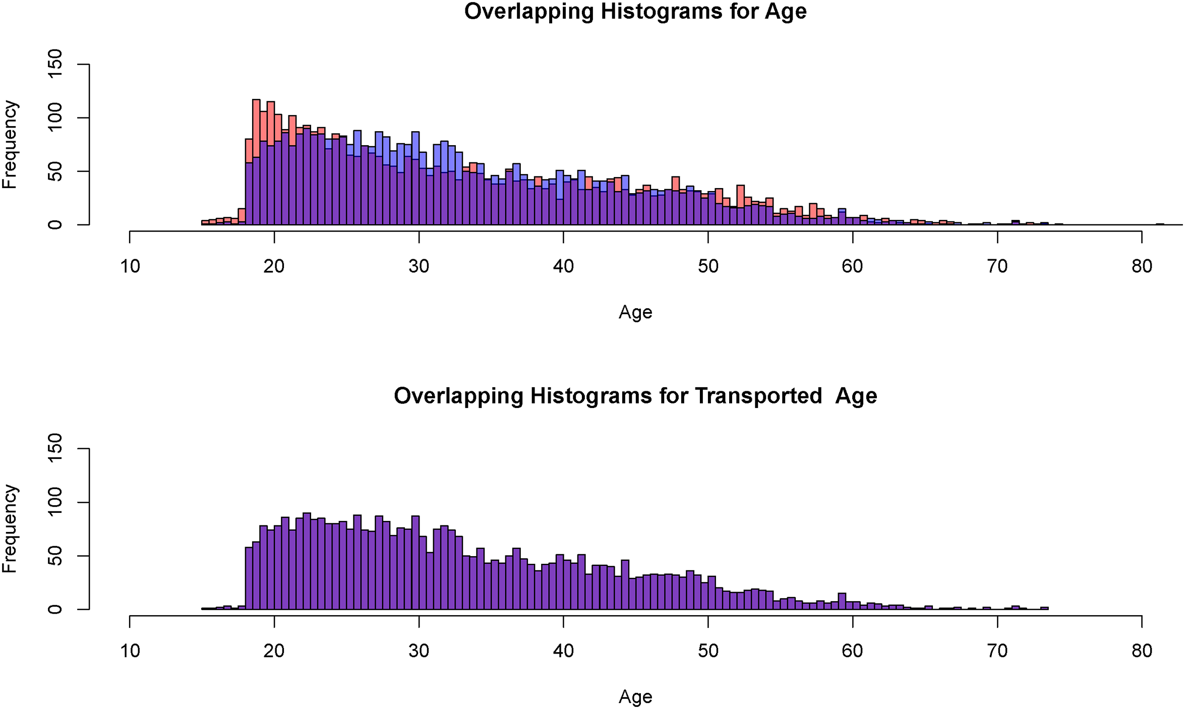
Histograms for an offender’s age and transported age (Black offenders in orange, White offenders in blue, overlap in purple, $N=4000$ ).

One must be clear that Figure 3 shows how the age distribution for the White test data and the Black transported test data are made virtually indistinguishable. We emphasize that this does not imply exact one-to-one matching of Black offenders to White offenders in units of years. Figure 3 results from a linear programming solution in which, as noted earlier, the squared distances between observations from the two joint covariate distributions in predictor space are minimized subject to fixed marginal distributions. More details are provided in the online Appendix C.

The performance of optimal transport in the bottom histogram may seem too good to be true. However, despite some distributional differences in the top histogram that may matter for risk, the overall shape of the two distributions is very similar. Both peak at low values and gradually decline in an almost linear fashion toward a long right tail. One should expect optimal transport to perform well under such circumstances.

Perhaps more surprising is that the two distributions are so similar to begin with. But arrests are a winnowing process that can affect members of protected classes in similar ways. The pool of individuals who are arrested is more alike than the overall populations from which they come. Regardless of race, the pool disproportionately tends to be young, male, unemployed, and unmarried, with appreciable previous police contact. It is commonly said that less than 10% of the overall population is responsible for more than 50% of the crime (e.g., Nath 2006) This disparity is reflected in the backgrounds of individuals who are arrested, coming more likely from that 10%.

Figure 4, constructed from the same 4000 observations, shows the results for an offender’s number of prior arrests for crimes of violence, which is also known to be associated with post-arraignment violent crime. It is apparent in the top histogram that Black offenders have more priors up to about 40, at which point there are too few cases to draw any conclusions. After the application of optimal transport, the bottom histogram shows no apparent differences. As before, the two distributions were not dramatically different before optimal transport was applied.

Figure 4.

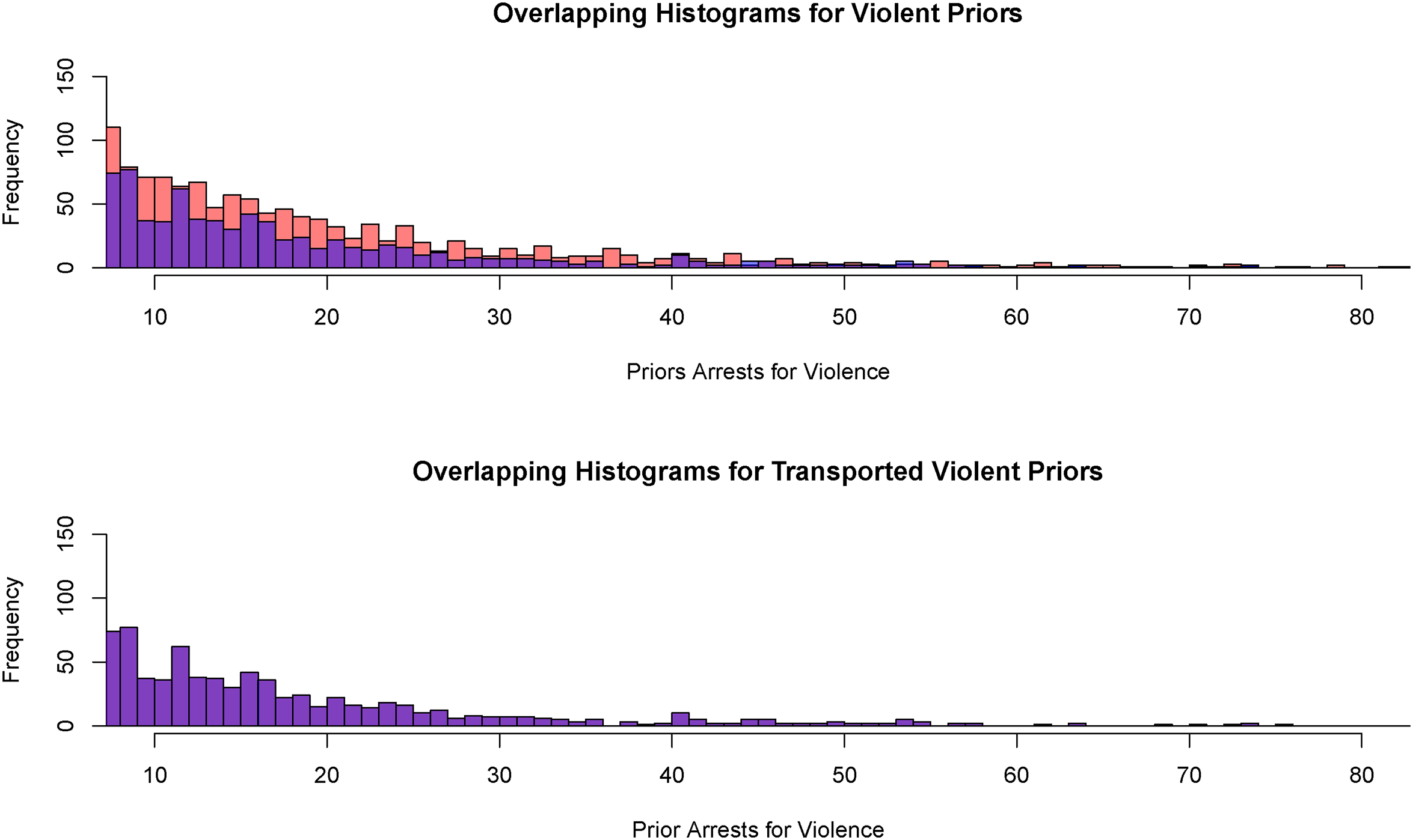
Histograms for the number of prior arrests for a crime of violence and the transported number of prior arrests for a crime of violence (Black offenders in orange, White offenders in blue, overlap in purple, $N=4000$ ).

Figure 5, using the same 4000 observations, shows the results for the earliest age at which an offender was charged as an adult. Offenders who start their criminal activities at a younger age are more crime-prone subsequently. From the top histogram, Black offenders are more common than White offenders at younger ages. That disparity disappears in the bottom histogram after optimal transport is applied, no doubt aided by the similar shapes of the two distributions. Optimal transport seems to perform as hoped to remove racial disparities in the two joint predictor distributions.

Figure 5.

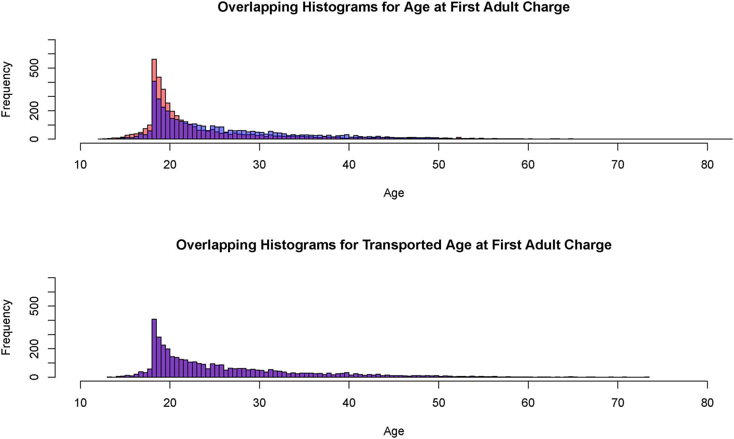
Histograms for the age of the first adult charge and the transported age of the first adult charge (Black offenders in orange, White offenders in blue, overlap in purple, $N=4000$ ).

But, the effectiveness of optimal transport in a forecasting setting remains to be addressed. We converted the transported joint predictor distribution constructed from the Black offender test data into conformal scores like those used in forecasting. The classifier trained on White offenders was tasked with producing the probabilities of an arrest for a violent crime. These probabilities were then subtracted from “1” and from “0,” yielding Black offender conformal scores for the two possible outcome classes. In other words, we were proceeding for illustrative purposes as if the Black test data were unlabeled, just as new data would be when forecasts are needed. Conformal prediction procedures for more than two outcome classes can be found in Kuchibhotla and Berk (2021).

The two conformal score distributions, one for the forecasted 1s and one forecasted 0s, were then compared to the White offender conformal scores computed in the same manner from the White test data (i.e., as if the data were unlabeled). Ideally, there would be no apparent racial differences.

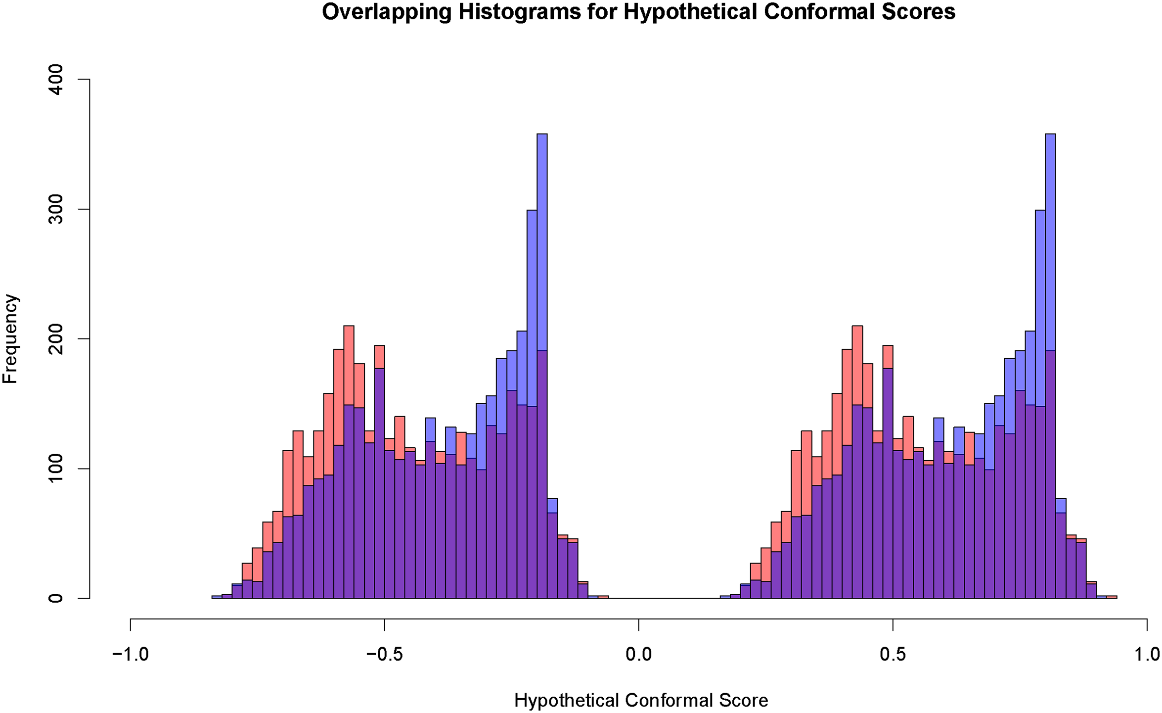
Figure 6 shows the results. The histogram to the left contains the conformal scores for cases in which the hypothetical outcome is no arrest for a crime of violence. The histogram to the right contains the conformal scores for cases in which the hypothetical outcome is an arrest for a crime of violence. As before, the histogram rectangles for Black offenders are in orange, the histogram rectangles for White offenders are in blue, and the overlap rectangles are in purple. Both histograms are entirely purple. The test data distribution of conformal scores for White offenders and Black offenders are for all practical purposes the same. ²¹ The claim is strengthened that for classifiers trained on White data, conformal prediction parity might be improved by optimal transport.

Figure 6.

Histograms for White conformal scores and transported Black conformal scores (Black offenders in orange, White offenders in blue, overlap in purple, $N=4000$ ).

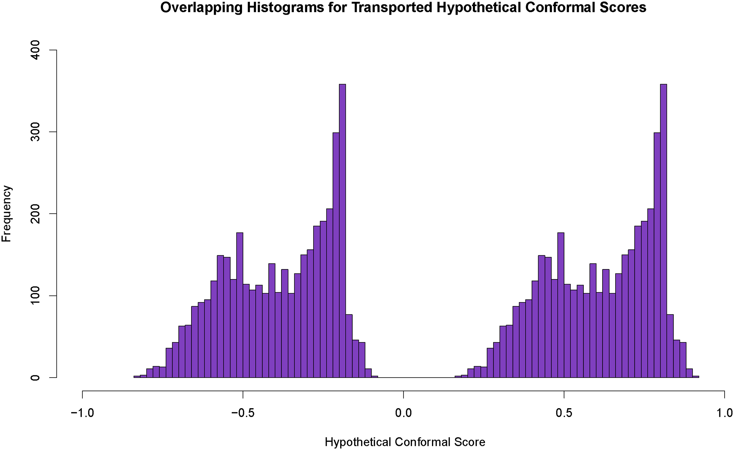
When actual forecasts are required, there is another step. For Black offenders, one needs a procedure that converts the predictor values for each unlabeled case into its corresponding transported values. These new cases were not available for the earlier optimal transport exercise, and repeating optimal transport for each new unlabeled case was at least impractical. Hütter and Rigollet (2020) instead suggest fitting a multivariate nonparametric smoother and using that to get good approximations of transported conformal scores. An added benefit is that the full range of predictor values for the unlabeled data can have comparable transported values. We applied random forests. ²²

One begins with a conventional $n\times p$ matrix of the original joint predictor test data distribution for Black offenders denoted by $X_b^{Test}$ . One also has an $n\times p$ matrix of the transported joint predictor distribution for Black offenders denoted by $X_b^{Trans}$ . Each column of $X_b^{Trans}$ is regressed in turn on $X_b^{Test}$ . Here, that means repeating this operation 21 times. Subsequently, the predictors for any unlabeled case could be used as input for the fitted random forest to output approximations of each transported predictor. These are then collected in a matrix denoted by ${\hat{X}}_b^{Trans}$ . When conformal scores for forecasting are needed, these approximations can be employed as usual as if they were the actual transported predictor values.

There is evidence from Figure 7 that some of the overlap in Figure 6 is lost because of the random forest approximation. For both histograms, Black offenders are somewhat overrepresented at smaller values, and White offenders are somewhat overrepresented at larger values. The performance of optimal transport has been degraded. If a conventional prediction region were imposed, Black offenders might be more commonly forecasted to be arrested for a violent crime, and White offenders might be more commonly forecasted not to be arrested for a violent crime.

Figure 7.

Histograms for White conformal scores and smoothed Black conformal scores with the 0 outcome label on the left and 1 outcome label on the right (Black offenders in orange, White offenders in blue, overlap in purple, $N=4000$ ).

The results might improve if our random forests application were better tuned or if some superior fitting procedures were applied. But, the conformal scores that matter for the contents of conformal prediction sets are only those that fall in the near neighborhood of the prediction region’s boundaries. Some may view this as a form of robustness. We need to consider whether in practice the reduction in overlap matters for fairness.

Evaluating Fairness in the Algorithmic Determinations of Risk

Recall that even after training the classifier only on White offenders, racial disparities remained. Especially relevant for this analysis is the lack of prediction parity. The apparent unfairness is caused by differences at arraignment between the joint predictor distributions for Black offenders and White offenders. We have shown that optimal transport can remove such disparities. But they are perhaps re-introduced when forecasts need to be made.

We have argued elsewhere (Kuchibhotla and Berk 2021) that when forecasting is the goal, accuracy is more usefully captured by conformal prediction sets than by confusion tables. One major problem with confusion tables is that forecasts are justified by minimizing Bayes loss even if there are very small differences between the estimated probabilities. For example, a distinction of 0.90 versus 0.10 for an arrest compared to no arrest, produces the same forecasted outcome category as a distinction of 0.51 versus 0.49. In other words, the reliability of the forecast is ignored, and an algorithm is forced to make a decision when perhaps it would be better to “defer” (Madras, Pitassi, and Zemel 2018). Another problem is that there are no finite sample coverage guarantees for confusion table forecasts, which can be problematic for real decisions when the number of cases is modest. Conformal prediction sets solve these problems and more.

Nevertheless, standard practice and many scholarly treatments of fairness emphasize examinations of confusion tables. We take a rather different approach through conformal prediction sets. In passing, interested readers can see in the online Appendix E that if one transports for Black offenders their joint distribution including the response variable as well the predictors, the confusion table from test data for White offenders is effectively the same as the confusion table from transported test data for Black offenders. For many stakeholders and some scholars, this may suffice for algorithmic fairness. This result should be reproduced in general. However, any conclusions are based on historical data which, as we have discussed, can be misleading for most kinds of fairness claims. We do not recommend this approach.

Results for Conformal Prediction Sets

We remain centered on prediction parity. For these data, predictive parity requires that conformal prediction sets for Black offenders and White offenders are substantially the same for a given coverage probability. Table 2 shows the results for our data on offenders at arraignment. A coverage probability was specified somewhat arbitrarily as $0.95$ . ²³

In order to obtain a sufficient number of observations for instructive results, we treated the test data for White and Black offenders as if the labels were unknown. For White offenders, we obtained conformal prediction sets as one ordinarily would. This is a very important feature of our procedures because it guarantees that our procedures do not alter the conformal prediction sets computed for Whites. Overall, therefore, White offenders as a protected class are not made worse off by the fairness adjustments because there are no such adjustments for White offenders.

For Black offenders, we proceeded in the same manner except using two different predictor distributions: for the transported, joint predictor distribution and for its random forests smoothed, transported approximation. For Black offenders, there were 4000 observations. For White offenders, there are about 10 times more.

The rows in Table 2 contain results for the four possible conformal prediction sets, where “1” denotes an arrest for a violent crime, and “0” denotes no such arrest. These prediction sets are shown in the first column on the left. In the second column are the proportions of times each prediction set materialized for the White test data. There were no empty sets implying that there were no outlier conformal scores. The most common prediction set was $\{0\}$ followed closely by $\{1,0\}$ . The prediction set $\{1\}$ surfaced very rarely. One might have expected these results because the outcome class of no arrest for a crime of violence dominated the marginal distribution of the response variable.

Table 2.

Estimated Proportions for Conformal Prediction Sets from White Test Data Predictors, Transported Black Predictors and Fitted Transported Black Predictors all at $1-\alpha =0.95$ .

Prediction	White	Black	Black
Set	Test Data	Transported Data	Smoothed Data
$\{\mathrm{\varnothing }\}$	0.0	0.0	0.0
$\{0\}$	0.58	0.58	0.54
$\{1\}$	0.03	0.03	0.03
$\{1,0\}$	0.39	0.39	0.43

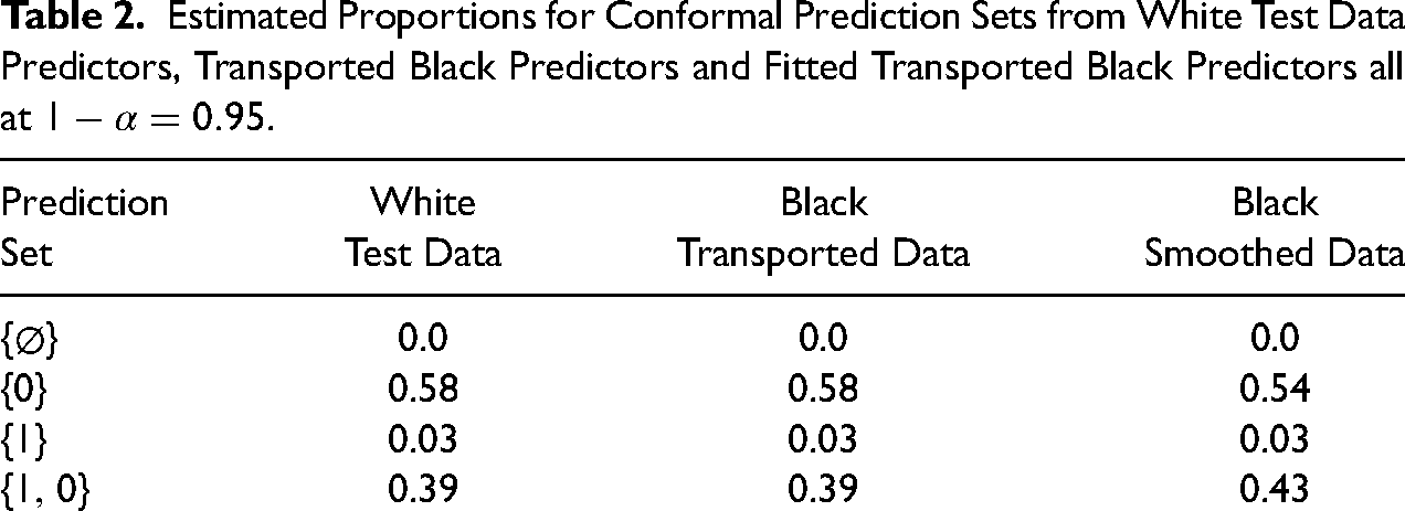
One important implication from the conformal prediction sets for Whites is that a substantial number of the arrest forecasts produced by the risk classifier and reported Table 1 might properly be seen as unreliable. The prediction set $\{1,0\}$ occurs nearly 40% of the time. 40% of the time, conformal prediction conveys that the two outcome classes cannot be reliably distinguished from one another. Yet, confusion tables nevertheless forecast a single outcome class.

The second and third columns have identical prediction set proportions for up to two decimal places; the prediction sets from the White offenders’ test data and from the Black offenders’ transported test data are effectively identical. One has prediction parity.

The fourth column shows that in practice there also is very close to perfect prediction parity when the approximate transported predictors are used for Black offenders. The proportion of prediction sets for which the forecast is an arrest for a violent crime remains at 0.03 for both Blacks and Whites. There is a slight reduction in the proportion of prediction sets that include no arrest by itself (i.e., $\{0\}$ ) and a slight increase in the proportion of prediction sets for which the classifier cannot make a clear choice (i.e., $\{1,0\}$ ).

Whether such differences matter would be for stakeholders to decide. A lot would depend on what a presiding magistrate would do with the $\{1,0\}$ prediction sets. An option that might be acceptable to all would be to withhold a decision until additional information was obtained that could improve forecasted outcome differentiation. In any case, we have demonstrated with real data on 300,000 arrested offenders at their arraignments that the provisional premise of White advantage compared to Blacks can be exploited to produce a very close approximation of prediction parity. Moreover, the class of Black offenders can be made better off while the class of White offenders is not made worse off.

Finally, there is no assurance that the comparability shown in Table 2 will be achieved in other settings. The number of observations matters. So do the properties of the data. We have produced prediction parity but have not guaranteed it for new data. It remains to be seen how widely our results might generalize. The challenge comes not just from different mixes of offenders, but from different ways to define “similarly situated.” Should juvenile arrests, for example, not be used? ²⁴

Discussion

The statistical principles used in our fairness formulation are easily generalized. We have already noted that a wide range of classifiers can be used in training and that one is not limited to binary outcomes. Across the range of statistical tools employed, there are also tuning parameters that can be varied depending on the nature of the data and the setting. For example, the value of the coverage probability for conformal prediction sets can trade-off uncertainty against the number of outcome categories likely to be included in the prediction set.

One is not limited to one disadvantaged, protected class. The analysis will be somewhat more involved, but for instance, one might treat Black offenders and Hispanic offenders as if they were White offenders. The limiting consideration will likely be a subject-matter rationale. Just as for Black offenders, there is substantial heterogeneity among Hispanic offenders (e.g., those of Cuban versus Puerto Rican descent). What matters is what impact that heterogeneity has on treatment by the criminal justice system and whether there are legal consequences for protected classes. For example, country of origin might well matter, but probably not marital status. One must not forget that the relevant perceived group differences between offenders usually are social constructions.

One also is not limited to training on a single protected class as the baseline. One can include two or more demographic classes insofar as that can be justified in subject-matter terms. In some jurisdictions, the advantaged demographic class might include White offenders and Asian offenders. One can also be more granular. For example, the advantaged demographic class might be Whites and Asians from affluent zip codes. However, there can be jurisprudential and political issues if the inclusion criteria are novel or contradict accepted practice.

As a technical matter, one can choose any subset of offenders to set the training baseline. However, important features of our approach can be compromised. For example, the outcome on which the training is done should be accepted as reasonably fair or the classifier will build in unacceptable unfairness. Such concerns are relevant even if only some of the training cases are treated unfairly by the criminal justice system. That is one reason why one might choose not to train on both Black and White offenders.

But the issues can be subtle and difficult to resolve. Might one be prepared to argue, for example, that if offenders were selected solely from affluent zip codes, race no longer matters? Could one sensibly train on affluent Whites and Blacks? And if so, is the range of offenses and covariate values adequate to permit sufficiently accurate risk assessments for individuals from far less affluent zip codes? Gang membership, for instance, might only be a risk factor in low-income neighborhoods and would be statistically overlooked if training were undertaken only with offenders from moderate to high-income neighborhoods. To repeat a recurring theme, the analysis must be constructively shaped by subject-matter and jurisprudential expertise.

Finally, one can easily imagine improving the data, the classifier, and conformal prediction set tuning such that a risk algorithm for White offenders has enhanced performance. That might lead to increased privilege for Whites and ordinarily could enlarge a White/Black fairness gap. But our approach to fairness would confer those very same advantages on Black offenders. Then, both protected classes can be made better off. It would be misguided to train instead on the less privileged group and transport the covariates of the more privileged group. One would have a group Pareto “loss” making the more privileged group less well off while not improving the lot of the less privileged group.

Conclusions

We have focused on the input and output of algorithmic risk assessments. Although any subsequent decisions or actions may be unfair, they are beyond a risk algorithm’s reach and are best addressed by reforms tailored to those phenomena. Blaming a risk algorithm is at best a distraction and can divert remediation efforts away from more fundamental change.

We have shown empirically that, at least for our data, prediction parity as a form of group fairness is easily achieved for a sensible risk baseline by (1) training on a more privileged protected class and then (2) transporting the joint predictor probability distribution from a less privileged protected class to the joint predictor probability distribution of a more privileged protected class. Pareto improvement at the level of protected classes can follow. The more privileged class is not made worse off. This also holds for the less privileged class that can be made better off as well. One might then argue that the risk algorithm dice are no longer loaded to favor one protected class over another. This strikes directly at concerns about mass incarceration and its many consequences.

By achieving prediction parity, we marshal support for the use of privilege as an organizing framework for internal fairness. We readily acknowledge the many unresolved questions about the precise content and meaning of “privilege,” especially in criminal justice settings, but whatever its nature, when a risk algorithm treats Black offenders as if they are White offenders, prediction parity can directly follow.

At the same time, we can make no claims about external fairness: classification parity, forecasting accuracy parity, and cost ratio parity. This is surely disappointing, but simply reflects the limitations of historical data when a fair risk algorithm is being sought. In other recent work (Berk, Kuchibhotla, and Tchetgen Tchetgen 2022), there are interesting ideas for how progress might be made by explicit framing of the risk algorithm’s development as a causal intervention in the decision-making status quo.

Likewise, there are limitations to what fair risk algorithms can accomplish and to the group Pareto optimality that results. Because of concerns about pervasive criminal justice unfairness, it may be tempting to inflate our claims. We have focused on algorithm fairness itself and the resulting group Pareto optimality. There are no broader contentions about the effects on criminal justice decisions or actions that follow. For example, we do not require that the algorithm increase the fairness of prosecutorial charges or the sentences given by judges to the offenders who later are convicted of those charges. Moreover, even if there were such downstream effects, they would not make the fair risk algorithm itself more or less fair. Finally, just as for virtually any public policy, there are no guaranteed safeguards against subversion, even if easily identified. For example, if at sentencing a judge, seeking to improve individual fairness, chose to introduce new offender features not used by the classifier (e.g., a sincere show of contrition), a fair risk algorithm may lead downstream to unfair outcomes, and a Pareto improvement might well not materialize. But the algorithm itself remains fair.

We also recognize that by intervening on behalf of members of less privileged protected classes, we concurrently introduce a form of differential treatment. This has a long and contentious fairness history. But in most such circumstances, some protected classes arguably are made better off as other protected classes arguably are made worse off. Our approach to criminal justice risk assessment can sidestep such concerns. Still, Pareto improvement for protected classes must pass political and legal muster. One hurdle is whether under our approach real and consequential injuries can be avoided (Lujan v. Defenders of Wildlife 1992); in U.S. federal court, “injury in fact” is mandatory. Another hurdle is whether there would be violations of “equal protection” under the 5th and 14th amendments to the U.S. Constitution (Coglianese and Lehr 2017: 1191–1205), despite our intent to make equal protection more equal. We are explicitly using race in our adjustments for fairness by training only on White offenders and transporting the Black covariate distribution to the White covariate distribution. The jurisprudential issues are surprisingly subtle, but the use of race in this manner actually might survive judicial scrutiny (Hellman 2020).

Finally, there can be concerns about proposing risk procedures, even if rigorous, that explicitly respond to criminal justice realpolitik. But current reform efforts are too often mired in misinformation and factional maneuvering, neither of which improve the public discourse. In contrast, our foundational premises are plain. Past research is consulted. The limits of our methods are explicit. And, we have shown with real data that they can be successfully applied.

Supplemental Material

sj-pdf-1-smr-10.1177_00491241231155883 - Supplemental material for Improving Fairness in Criminal Justice Algorithmic Risk Assessments Using Optimal Transport and Conformal Prediction Sets

Supplemental material, sj-pdf-1-smr-10.1177_00491241231155883 for Improving Fairness in Criminal Justice Algorithmic Risk Assessments Using Optimal Transport and Conformal Prediction Sets by Richard A. Berk, Arun Kumar Kuchibhotla and Eric Tchetgen Tchetgen in Sociological Methods & Research