Sage Journals: Discover world-class research

Abstract

Discrete-time survival analysis (DTSA) models are a popular way of modeling events in the social sciences. However, the analysis of discrete-time survival data is challenged by missing data in one or more covariates. Negative consequences of missing covariate data include efficiency losses and possible bias. A popular approach to circumventing these consequences is multiple imputation (MI). In MI, it is crucial to include outcome information in the imputation models. As there is little guidance on how to incorporate the observed outcome information into the imputation model of missing covariates in DTSA, we explore different existing approaches using fully conditional specification (FCS) MI and substantive-model compatible (SMC)-FCS MI. We extend SMC-FCS for DTSA and provide an implementation in the smcfcs R package. We compare the approaches using Monte Carlo simulations and demonstrate a good performance of the new approach compared to existing approaches.

Keywords

Multiple imputation event analysis survival analysis missing data fully conditional specification family research smcfcs

Introduction

Many phenomena in the social and medical sciences can be characterized as events—that is, qualitative changes that occur at some point in time. Typical research questions focus on whether, when, and under what circumstances events occur. Examples of sociologically relevant events are divorce or a job offer after a period of unemployment. When analyzing such time-to-event (or survival time) data, one cannot rely on a simple linear regression model, as the event cannot be observed—it is missing (censored)—for parts of the population. For example, some married people never experience divorce, and although everybody dies, data collection will almost certainly not continue until this point for all observations. Different analytical approaches have been developed to deal with the censoring problem. They include, for example, Cox regression for continuous-time survival analysis (Cox, 1972). Cox (1972) also extended the proportional hazard model for discrete-time survival analysis, analyzing the conditional odds of an event occurring at a particular time point, given survival up to that point. For discrete-time survival analysis, data must first be converted from the familiar person-oriented (P) format (one row for each person/observational unit) to a person-period (PP) format (one row for each time period in which a person was observed).

One challenge that arises in the application of these survival models (and in other models) is that often one or more covariates have missing data. Simplistic approaches, such as listwise deletion (LD) and unconditional mean imputation, are still used in the social sciences (e.g. Böttcher, 2006; Cooke, 2006; Arránz Becker and Lois, 2010; Manning, Brown, and Stykes, 2016; Cooper et al., 2018; Stoddard and Veliz, 2019). However, these approaches may be highly inefficient or lead to severely biased variance estimates. Point estimates may also be biased after LD if missingness depends on the outcome (Hughes et al., 2019).

Another approach to handling missing data is multiple imputation (MI) (Rubin, 1987, 1996; Schafer, 1997; van Buuren, Boshuizen, and Knook, 1999). MI leads to unbiased point and variance estimates if certain conditions concerning the missing data mechanism and the imputation model are met (Allison, 2000). However, while there has been researching on how best to impute missing covariate values for Cox regressions (van Buuren, Boshuizen, and Knook, 1999; Clark and Altman, 2003; White and Royston, 2009; Keogh and Morris, 2018), the Cox cure model (Beesley et al., 2016) and the relative survival model (Nur et al., 2009), the imputation of covariates in discrete-time survival analysis is still understudied. For time-varying covariates, Murad et al. (2019) showed that MI approaches using information from the previous and current time points seem sufficient in most situations. However, in discrete-time survival analysis, not only time-varying covariates but also time-invariant covariates are used. This article contributes to the literature by exploring how to specify a suitable imputation model for partially missing time-invariant covariates in discrete-time survival analysis. We present different approximations and an approach using a compatible imputation model now implemented as smcfcs.dtsam in the R package smcfcs.

This is not an easy or straightforward task. Kenward and Carpenter (2007: 207) shows that including outcome information in the imputation model for partially observed covariates is crucial for unbiased estimates. However, with discrete-time survival models, the time-to-event is not fully observed due to censoring. Nor is it clear in which format the imputation procedure should be carried out: with data in P or PP format? And how should the relationship between the time-to-event variable and the covariates be modeled for imputation?

These are relevant issues, as discrete-time survival analysis is widely used in the social sciences, especially in family sociology (see, e.g., Barber, 2001; Schoen et al., 2002; Cooke, 2006; Nomaguchi, 2006; Arranz Becker and Lois, 2013), and also in the medical sciences (Murad et al., 2019).

The remainder of this article is organized as follows: In the next section, we introduce the formalization of the discrete-time survival analysis model (DTSAM) proposed by Singer and Willett (2003), we address P and PP data set formats, and we briefly discuss the negative consequences of, and ways of dealing with missing covariate data. We then outline the method of MI and present several possible imputation approaches that differ in terms of the data format used and the specification of the imputation model, including a new substantive-model compatible-fully conditional specification (SMC-FCS) approach for DTSAMs implemented in the function smcfcs.dtsam in the R package smcfcs. Following this, we conduct four simulations with discrete-survival data and varying degrees of unobserved heterogeneity, also called frailty (McGilchrist and Aisbett, 1991). Using data from the German Family Panel (pairfam), we then provide an applied example with real-world data. The article concludes with a discussion of the results and further steps.

Discrete-Time Survival Analysis Model

The Model

In this section, we introduce the formalization of a DTSAM proposed by Singer and Willett (1993).

The term discrete survival is used when the time-to-event can take only distinct values, for example, one, two, three, or more years/semesters/weeks. Occasionally, discrete-survival data are “truly discrete” (Kleinbaum and Klein, 2012: 325); that is, the event can occur only at distinct values of time (e.g., fertility modeling, particularly the time from puberty to first childbirth). However, in most cases, discrete data are the result of interval-censoring: events might happen in a continuous range of time, but they were observed only in grouped form instead of continuous-time data—for example, the year of divorce is recorded but not the month and day (Kleinbaum and Klein, 2012: 318).

Following Singer and Willett (1993: 163), let $T$ be a discrete random variable that indicates the time period $j$ when the event occurs for a randomly selected individual from the population. For example, $T$ could be the time until divorce in a person’s first marriage. Note that we focus here on non-repeatable events, and that event occurrence is thus inherently conditional. For instance, a person can experience the divorce of their first marriage only if he or she did not already experience it in any of the periods prior to $j$ . We aim to describe $T$ by a conditional probability mass function. The conditional probability that an event will occur in each period given that it has not occurred earlier is called the discrete-time hazard, $h_{j}$ .

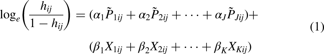
Researchers are usually interested in whether the risk of event occurrence differs systematically between observations. For example, in a study of divorce risks, the risk might depend on age at the beginning of a marriage or on differences in social status between the spouses. For now, we examine time-invariant predictors. We have to distinguish between different individuals $i$ , each with their predictor values $X_{k i}$ for $K$ ( $k = 1, \dots, K$ ) predictors $X_{k}$ .

We model the individual hazard $h_{i j}$ as depending on a set of indicator variables ${\tilde{P}}_{j}$ for all time periods $j$ ( $j = 1, \dots, J$ ) and predictors $X_{k}$ through a logit link (Cox, 1972; Allison, 1982; Singer and Willett, 1993). The tilde indicates that we have a binary indicator for a specific time period instead of the numeric variable with the number of the period.

The model to be estimated is that proposed by Singer and Willett (2003: 317):

\begin{aligned} \log_{e} (\frac{h_{i j}}{1 - h_{i j}}) & = (α_{1} {\tilde{P}}_{1 i j} + α_{2} {\tilde{P}}_{2 i j} + \dots + α_{J} {\tilde{P}}_{J i j}) \\ (β_{1} X_{1 i j} + β_{2} X_{2 i j} + \dots + β_{K} X_{K i j}) \end{aligned}

(1)

This model contains no single stand-alone intercept, but rather a set of alpha parameters

[α_{1}, α_{2}, \dots, α_{J}]

, each of which acts as an intercept for a specific time period.

[{\tilde{P}}_{1 i j}, {\tilde{P}}_{2 i j}, \dots, {\tilde{P}}_{J i j}]

are a sequence of indicator variables which indicate the time periods.

J

represents the last time period observed for anyone in the sample. The period indicator for the first periods takes the value 1 for a unit if

j = 1

and 0 for all other values of

j

. The

β

s indicate how much the logit-hazards shift with a unit shift in the parameters—for example, how much an additional year in age difference between partners shifts the logit of the hazard of divorce.

[X_{1 i j}, X_{2 i j}, \dots, X_{K i j}]

are covariates that can include both time-invariant as well as time-varying covariates. Time-invariant covariates will of course only vary between units and not within a unit between different periods. In this article, we will focus on time-invariant covariates.

The Data: Transformations and the Person-Period Format

Having established our model, we take a closer look at our data and the data format needed for a DTSAM. Data are typically available in a P format, with one row (record) for each observational unit (i.e., person). Apart from the covariates, $X_{k}$ , there are three possible outcome variables. First, there is the variable $T$ , that is, the time-to-event. However, in most applications, we would almost certainly have a lot of missing data in $T$ due to censoring. Usually, therefore, instead of the variable $T$ , the variable $Y$ —the last period in which a unit was observed—is used. This variable is observed regardless of whether the event occurred or censoring happened. We also add a dichotomous event indicator, $E$ , set to one if the event occurred and to zero if the observation is censored.

To estimate a DTSAM (our substantive model), the P data set must be converted into a PP format (Singer and Willett, 1993: 172). In PP format (see Table 1), there is a separate row for each period in which a unit was observed. Apart from the covariates, we usually have observed period indicators into indicator variables ${\tilde{P}}_{j}$ for every period $j$ ( $j = 1, \dots, J$ ) and an event indicator, $E$ . The event indicator is set to one only if the event occurred for this unit in this specific period. Although the last period in which a unit was observed, $Y$ , is not usually included separately in PP format, we will need it for certain imputation approaches. $Y$ as an added variable in PP format is exclusively used for imputation, not for analysis.

Table 1.

Exemplary data set in person-period (PP) format.

Obs	$X_{1}$	$X_{2}$	$X_{3}$	$X_{4}$	$X_{5}$	$P$	$E$	$Y$
1	9.3	3	Female	Rural	6	1	0	4
1	9.3	3	Female	Rural	6	2	0	4
1	9.3	3	Female	Rural	6	3	0	4
1	9.3	3	Female	Rural	6	4	1	4
2	4.1	2	Male	Urban	3	1	0	6
2	4.1	2	Male	Urban	3	2	0	6
2	4.1	2	Male	Urban	3	3	0	6
2	4.1	2	Male	Urban	3	4	0	6
2	4.1	2	Male	Urban	3	5	0	6
2	4.1	2	Male	Urban	3	6	0	6
3	2.1	4	Male	Urban	4	1	1	1
$\dots$	$\dots$	$\dots$	$\dots$	$\dots$	$\dots$	$\dots$	$\dots$	$\dots$
$\dots$	$\dots$	$\dots$	$\dots$	$\dots$	$\dots$	$\dots$	$\dots$	$\dots$
n	$\dots$	$\dots$	$\dots$	$\dots$	$\dots$	$\dots$	$\dots$	$\dots$
n	$\dots$	$\dots$	$\dots$	$\dots$	$\dots$	$\dots$	$\dots$	$\dots$

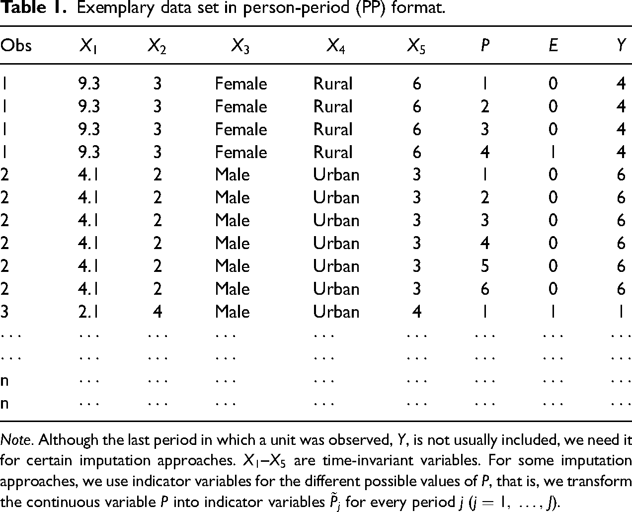
Note. Although the last period in which a unit was observed, $Y$ , is not usually included, we need it for certain imputation approaches. $X_{1}$ – $X_{5}$ are time-invariant variables. For some imputation approaches, we use indicator variables for the different possible values of $P$ , that is, we transform the continuous variable $P$ into indicator variables ${\tilde{P}}_{j}$ for every period $j$ ( $j = 1, \dots, J$ ).

The dichotomous event indicator, $E$ , is treated as a collection of independent values with a hypothesized logistic dependance on predictors (Singer and Willett, 1993: 174). If one interprets model coefficients on an individual level, one implicitly asserts that the variables exhaust all the sources of individual variation in the hazard rate, that is, that the variation in hazards is due only to differences in the independent variables and periods, and that the model is correctly specified. The survival model literature describes these models as having no unobserved individual heterogeneity (Allison, 1982: 82). A major concern of many statisticians is to handle variation between individuals, usually through the inclusion of covariates in analyses. However, a number of variables will not be measured or may be totally unobservable with a current methodology or in general. This unobserved individual heterogeneity, also called frailty (Vaupel, Manton, and Stallard, 1979; Aalen, 1994), is an important problem in survival analysis.

The omission of a critical predictor of the outcome from the model is equivalent to mixing hazard profiles for the different populations defined by the discarded predictor values, that is, the hazards converge. The pooled converged hazard profile does not have to look like any member of the general population. For example, assume that all members of the population have a constant hazard over time, but the height of the risk profile differs between members. Over time, members with a high risk drop out of the population. If we do not include the predictor that shifts the members’ risk, the aggregate profile will show a risk profile that decreases with time (Singer and Willett, 1993: 185).

Building a model that exhausts all sources of individual variation is practically not feasible. However, even in the absence of important predictors, parameters can still be interpreted as an average across population hazard profiles (Xue and Brookmeyer, 1996). For example, if we include obesity as a risk factor for diabetes in our model, and there is unobserved individual heterogeneity, we would estimate the log odds ratio for all people with obesity versus those without. If there were no unobserved heterogeneity, we could interpret the regression coefficient as the log odds ratio for an individual before versus after developing obesity. Apart from complicating the interpretation of factors, Allison (1982: 83) also noted that in the case of frailties, “one would expect this dependance among the observations to lead to inefficient coefficient estimates and standard errors that are biased downward.” As unobserved heterogeneity is not entirely avoidable, we will generate the data sets in our simulations with varying degrees of unobserved heterogeneity. However, before testing the different MI approaches, we take a closer look at the implications of missing data for discrete-time survival analysis.

Implications of Missing Data for Discrete-Time Survival Analysis

Surveys are often subject to missing data, and we have to decide how to treat partially observed covariates in discrete-time survival analysis. Note that, in this article, we are looking only at missing data in the covariates, not in the time-to-event variable.

Before exploring different possible strategies for imputing partly missing covariates in discrete-time survival analysis, we take a more general look at the implications of missing data in regression analysis to demonstrate the need for a suitable MI strategy.

One way to deal with missing data in regression analysis is to exclude incomplete observations. This is known as LD or complete case analysis. One consequence of this approach is a possibly considerable loss of efficiency or information (Carpenter and Kenward, 2013: 9) as only the observations with complete records are used. In other words, even if only one of many covariates is missing, this leads to the complete exclusion of the observation. This becomes especially problematic if the aim is to keep unobserved heterogeneity down and include not only possible confounders but also other important predictors that explain significant parts of the variation.

However, a loss of efficiency, or information, is only one side of the coin; the other is bias. Table 2 gives an overview of the conditions under which logistic regression coefficients will be biased after LD. Here, $X_{1}$ and $X_{2}$ are two independent variables, and $Y$ is the dependent binary outcome variable. For now, only the variables on which the completeness of a case depends (e.g., the outcome and $X_{1}$ ) are of relevance, not the type of missingness mechanism that is behind the nonresponse.

Table 2.

Bias in case of logistic regression using complete records.

Mechanism	Biased Coefficients?
depends on	Constant	Coeff. $X_{1}$	Coeff. $X_{2}$
$Y$	Yes	No	No
$X_{1}$	No	No	No
$X_{2}$	No	No	No
$X_{1}$ , $X_{2}$	No	No	No
$Y$ , $X_{1}$	Yes	Yes	No
$Y$ , $X_{2}$	Yes	No	Yes
$Y$ , $X_{1}$ , $X_{2}$	Yes	Yes	Yes

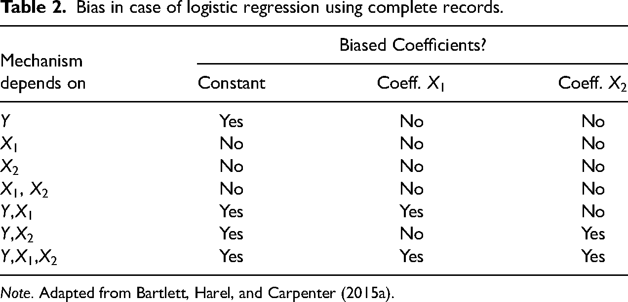
Note. Adapted from Bartlett, Harel, and Carpenter (2015a).

Complete case analysis is valid for linear and logistic regression if missingness depends on the covariates but not the outcome, which in the situation considered here means missingness could depend on $X_{1}$ and $X_{2}$ (or only one of the two covariates) but not $Y$ . From Table 2, we can further read that in the case of logistic regression—for example, the DTSAM—the coefficient estimate of an independent variable $X_{1}$ after LD is biased only if the completeness of an observation depends:

on the binary outcome $Y$ and

on the covariate $X_{1}$ itself (Carpenter and Kenward, 2013; Little, 2019).

Therefore, if it must be assumed that the estimated coefficient of our variable

X_{1}

will be biased after LD, other approaches to handling missing data are needed. Nevertheless, even if we are confident that our analysis will not be biased after LD, we will lose information from incomplete cases. Thus, LD cannot be an adequate solution in most cases, and we will look into MI as a possible remedy for these unwanted effects of missing data.

Multiple Imputation

MI in General

One of the most popular approaches to tackle missing data is MI (Little and Rubin, 2002). MI allows for the analysis of incomplete data sets by substituting missing values. Substitution is performed by imputing values of a variable based on other variables, mostly those of the analysis model. In the analyses, these imputed values are not treated the same as observed values, as this would lead to biased variance estimates. Therefore, several values instead of just one are imputed for each missing value in order to avoid treating imputed values as observed. Each data set is then analyzed separately, and estimates and variances are combined across imputations using rules developed by Rubin (1987).

To impute missing values, we need models of their distribution. There are two main approaches, joint modeling (JM) and FCS, also known as multivariate imputation by chained equations or MICE (van Buuren, 2007).¹ Joint modeling MI (Schafer, 1997) draws missing values simultaneously for all incomplete variables using a multivariate distribution. However, specifying such a joint model is often challenging, for example, if there are both continuous and discrete variables with partially missing information in a data set. Newer approaches now allow us to specify the models for each variable one at a time, for example, Erler, Rizopoulos, and Lesaffre (2021). FCS divides the problem into a series of univariate problems (van Buuren, 2007). FCS involves specifying a series of univariate models for the conditional distribution of each partially observed variable, given all the other variables (White, Royston, and Wood, 2011). It is more flexible than the JM approach because adequate regression models can be selected for every variable (e.g., linear regression for continuous partially observed variables, logistic regression for binary partially observed variables). However, for FCS, the joint distribution of variables is only implicitly known and may not actually exist. While this is a serious drawback from a theoretical perspective, it has done little harm to practical application.

When specifying the imputation model, it is crucial to account for the substantive model of interest—which is often also called the analysis model. The associations to be examined in the substantive model must also be represented in the imputation model. Otherwise, bias toward zero will be the likely consequence (Fay, 1992). The imputation and substantive models should be compatible. Compatible means that there exists a joint model with conditionals corresponding to the imputation and substantive models (see Bartlett et al., 2015b and for the related term of congeniality see Meng, 1994). In addition to JM and FCS, a variation of FCS that allows one to more easily specify a compatible imputation model was developed by Bartlett et al. (2015b). It is called SMC-FCS. SMC-FCS is used when it is hard to find a compatible standard FCS imputation model because the substantive model, that is, the model the researcher is interested in, is either non-linear (e.g., a Cox regression) or contains non-linear (e.g., squared or interaction) terms. SMC-FCS can also be used for models without non-linear terms. As with FCS, separate models are specified for the partially observed variables. What differentiates SMC-FCS from regular FCS is that the conditional distribution of a variable (given the other variables) is combined with the specified substantive model to define an imputation model. This combination ensures that the missing covariate data are drawn from models compatible with the specified substantive model.

Handling Missing Covariates Values in Case of a DTSAM as a Substantive Model

Representing the associations in the substantive model of interest is not straightforward in the case of a DTSAM and its complicated outcome structure. Generally, we have two outcome variables: the event indicator, $E$ , and the last period in which a unit was observed, $Y$ (either because the unit was subsequently censored or the event occurred during that period). One also has to decide whether to impute in a P or PP format.

We will explore several imputation approaches that differ in terms of (1) the data format used, (2) the general imputation approach used, and (3) the imputation model specification. The data format in which we impute has two possible formats: P and PP format. We examine both FCS and SMC-FCS approaches. Our imputation models differ in terms of whether we include variables for different periods or (censored) survival times or whether we also treat the (uncensored) time-to-event, $T$ , as a partially observed covariate (Beesley et al., 2016) and impute conditional on this partially imputed variable. Most approaches are easy to implement through existing software such as the mice and smcfcs (Bartlett and Keogh, 2019) packages. We also propose and provide the derivations for a new SMC-FCS approach in-person format (see the online Appendix), which allows consistent, that is, the same imputed values for periods in a unit for time-invariant covariates. At the same time, the imputation model is compatible with the substantive model.

We want to note that our primary goal here is not to impute (censored) survival times but instead partially missing covariates for the estimation of survival regressions. MI is also helpful if researchers wish to estimate marginal survival distributions, for example. Still, in this article, we are not primarily concerned with imputing the dependent variable of the survival regression. Interested researchers can consult Carpenter and Kenward (2013: 177) for suitable imputation strategies or adapt the strategies proposed for partially classified categorical data in Chapter 13 of Little (2019).

FCS with Data in P Format

We begin with the imputation approaches in a P format, that is, before converting the data to a PP format. We present several approaches, some of which are taken from the literature on MI with continuous survival (cure) data (Beesley et al., 2016). They differ mainly in terms of the implemented conditioning on the (censored) time-to-event. For all imputation models presented, we also condition the other covariates. Imputation is performed using the R (R Core Team, 2019) package mice (van Buuren, 2007) with single-level normal imputation.

Let $X_{k}$ be one of $K$ incomplete continuous-time-invariant random variables ( $k = 1, \dots, K$ ) and let $X$ be $X = (X_{1}, \dots, X_{K})$ . Let $X_{- k} = (X_{1}, \dots, X_{k - 1}, X_{k + 1}, X_{K})$ . Let $Z_{m}$ be one of $M$ complete variables $(m = 1, \dots, M)$ and let $Z = (Z_{1}, \dots, Z_{M})$ . We discuss all imputation approaches regarding continuous-time-invariant random variables but since the difference between the methods lies in the general approach (FCS vs. SMC-FCS) and the included variables, the transfer to other variable types (binary, ordinal) is in principle easy. The actual performance is however an open question that has to be covered in subsequent research.

In the following, we will mainly discuss how to incorporate the information included in the event indicator, $E$ , as well as the last observed-period variable, $Y$ , or the uncensored but incompletely observed time-to-event variable, $T$ .

The first approach (FCS P $Y + E$ ) uses indicator variables ${\tilde{Y}}_{j}$ ( $j$ periods, $j = 1, 2, \dots, J$ ) for each possible period $j$ . Y is handled as a factor variable, that is, ${\tilde{Y}}_{j}$ takes the value 1 if $j$ is the last observed period. Let $\tilde{Y}$ be $\tilde{Y} = ({\tilde{Y}}_{1}, \dots, {\tilde{Y}}_{J})$ . The aim is to allow for enough flexibility in the relationship between $Y$ and the other covariates. If overparametrization is a concern, an alternative would be to drop predictors using a simple method such as stepwise selection.

The imputation model is:

X_{k} = [\tilde{Y}, E, X_{- k}, Z] β + e, e \sim N (0, I σ^{2})

(2)

with persons as observational units and

I

denotes the identity matrix.

This specification with indicator variables for each possible time point is flexible, but it is possible only if the number of discrete-time points is not too large, the hazard is not expected to be near zero in some periods, and the risk sets are sufficiently large for each time point. Other specifications of the relationship between (censored) time-to-event are possible in these cases. They include, for example, linear, quadratic, cubic, or higher-order polynomials. It is also possible to use the logarithm of time (Klein, Kopp, and Rapp, 2013) or step functions for grouped periods. For our simulation, however, we do not simulate more than 15 possible time points. Thus, we use indicator variables to keep the specification as general as possible.

Another approach in the P format (FCS P $l o g (T)$ ) is to treat the time-to-event, $T$ , as a partially observed covariate (Beesley et al., 2016; White and Royston, 2009), and thus to impute it in the same way as the partially observed covariates. We impute the partially observed covariates conditional on the other covariates and the logarithm of the observed and currently imputed values of the logarithm of the time-to-event, $l o g (T)$ , and not on the last period a unit was observed, $Y$ , and the event indicator, $E$ . $l o g (T)$ imputations are done with a normal model.

The imputation model is thus

X_{k} = [\log (T), X_{- k}, Z] β + e, e \sim N (0, I σ^{2})

(3)

with persons as observational units.

FCS with Data in PP Format

It is also possible to impute after converting the data to a PP format. Note that persons will receive varying imputed values for time-invariant covariates. As in the approaches in the P format, we always impute conditional on all other covariates. Imputation is again done with mice in R.

For our first approach (FCS PP $P + E$ ) in the PP format, we impute conditional on the event indicator, $E$ , and a set of indicator variables ${\tilde{P}}_{j}$ for all periods $j$ ( $j = 1, \dots, J$ ). The indicator variables are indicators in which time period the observation is currently.

The imputation model is thus

X_{k} = [\tilde{P}, E, X_{- k}, Z] β + e, e \sim N (0, I σ^{2})

(4)

with periods within persons as observational units.

However, we expect that we will lose important information, especially for the rows belonging to the first few periods. If we do not include the last period in which a unit was observed, $Y$ , we do not directly condition the censored survival time. We impute conditional on the actually observed endpoint (i.e., the last time observed and event indicator) but rather the binary endpoint just in that period.

Therefore, we also try imputing conditional on the last period in which a unit was observed instead of the current period. We use the set of indicator variables $\tilde{Y_{j}}$ (FCS PP $Y + E$ ) for all periods $j$ ( $j = 1, \dots, J$ ).

The imputation model is thus

X_{k} = [\tilde{Y}, E, X_{- k}, Z] β + e, e \sim N (0, I σ^{2})

(5)

with periods within persons as observational units.

SMC-FCS with Data in PP Format

After presenting several possible FCS approximations, we now examine possible SMC-FCS approaches in this setting. SMC-FCS has shown excellent results in different simulation settings (Bartlett et al., 2015b; Beesley et al., 2016). We explore how this approach fares with a DTSAM as a substantive model. In contrast to the other imputation approaches, we now have to include the substantive model.

When we include the substantive model (see equation (1)) using the R package smcfcs (Bartlett and Keogh, 2019) and impute in PP format (SMC-FCS PP $P + E$ ), we effectively condition our imputations on the current period, $P$ , of the row aside from the other covariates and the event indicator, $E$ . Therefore, the imputation model includes all variables that are also part of the substantive model of interest, and all the data are in the same format. However, the imputation model does ignore that in the original data set persons have the same value for all periods in the case of a time-invariant variable, and it is not using the information about whether the subject eventually is seen to have the event or not and when this takes place.

A New SMC-FCS Approach: SMC-FCS DTSAM

The approaches presented in the previous sections are all approaches that can easily be implemented in already existing imputation software such as mice or smcfcs. However, they all have at least one problematic feature; some are not compatible with the substantive model, or values are imputed when the data set is already in PP format. This leads to different values between periods observed for a single unit and is possibly undesirable and confusing for practitioners since time-invariant variables do not differ between periods for observed units. Moreover, the PP approaches which do not use the last period information do not condition on the full outcome information for each subject.

We therefore propose a new SMC-FCS approach for imputing partially observed covariates from models which are compatible with the DTSAM specified by the user. The new SMC-FCS DTSAM approach leads to imputated covariate values, which are time-invariant for each unit, as they should be. Its derivation, which extends the derivation given by Bartlett et al. (2015b) for continuous survival endpoints, is available in the online Appendix, and it is implemented as smcfcs.dtsam in the R package smcfcs. Like the regular smcfcs function for variables in the linear or logistic model, smcfcs.dtsam includes a rejection sampling step. Samples are drawn from a candidate distribution for the covariate that includes any fully observed variables in the substantive model and all partially observed variables except the one being imputed. If $X$ is the potentially observed covariate and $Z$ the fully observed one, we draw the candidate value $x^{*}$ from $f (X | Z)$ and $U \sim U (0, 1)$ and accept if $U \leq P (T = Y | X = x^{*}, Z)$ in the case of $E = 1$ . In the case of $E = 0$ , we accept if $U \leq P (T > Y | X = x^{*}, Z)$ . For the new smcfcs.dtsam function, these candidate values are drawn before transforming the data set from person format to PP format. This allows for time-invariant imputations for a unit, in contrast to the previous ad-hoc approach where we used the regular smcfcs function with data in PP format. We want to note that the data should be provided in person format instead of in PP format when using the smcfcs.dtsam function.

Simulation Study

Data-Generating Mechanisms

We now examine the performance of the imputation approaches in a series of four simulations. We first present the details (data-generating mechanisms, the introduction of missingness, performance measures) of the simulations and then discuss the results.

For all four simulations, we create five continuous covariates, $X_{k}$ $(k = 1, \dots, 5)$ , drawn from a multivariate normal distribution with means of 0 and variances of 1. The covariates are weakly correlated with each other ( $r = 0.1$ ).

Concerning the generation of the survival times, we use the DTSAM model (see equation (1)), which will be estimated after the introduction of missingness and the subsequent imputation. This yields (truly) discrete-survival data that fulfill the assumption of proportional odds for the DTSAM (Singer and Willett, 1993: 167), the substantive model of interest. When we do not add a frailty term to the generation of survival times, there is no unobserved heterogeneity when we refit the model that we used for data generation on the simulated data. However, as several authors have noted, it is hard to specify a model without omitting any frailty variables. Ideally, one would diagnose this misspecification and change the model to address this. But this is often not possible and unobserved heterogeneity is therefore present (Allison, 1982: 83). Therefore, no unobserved heterogeneity is simulated only in one of the four simulations. In the other three simulations, we simulate successively larger amounts of unobserved heterogeneity. In all three cases, the frailty term is normally distributed, with a mean of 0 and variance that increases between simulations (0.25, 1, and 4). We add the frailty term after creating the covariates, and before simulating survival times and transforming the data set from a person format to PP format. We use $α = (- 5.00, - 4.72, - 4.44, \dots, - 0.8)$ and $β = (0.8, 2.2, - 0.5, 0.3, - 1.4)$ as parameter vectors (see equation (1)). We simulate 15 possible time points; after the last time point, all observations are censored.

For each simulation scenario, we generate 1,000 simulated data sets with 2,000 persons each to prevent the Monte Carlo error from masking differences between methods. Data set length in PP format will vary.

Missingness

To introduce missingness in each of the simulations, we set 30% of observations missing in $X_{1}$ , $X_{2}$ , and $X_{3}$ , depending on $X_{4}$ , $X_{5}$ and $T$ with all coefficients for the missingness model drawn from $N (1, {0.5}^{2})$ . Therefore, the completeness of an observation row depends both on the outcome and the covariates, which leads to biased coefficient estimates after LD.²

After introducing different possible imputation strategies and creating data sets with missing observations, we are now able to examine the performance of the different imputation approaches.

Methods Compared and Performance Measures

We perform MI of partially observed covariates in discrete-time survival analysis using the imputation specifications described earlier in this article. For each simulation and method, we create five imputed data sets. We then compute the mean coefficient, relative bias, mean squared error (MSE), confidence interval (CI) length, and coverage for estimated DTSAM parameters across 1,000 Monte Carlo (MC) repetitions for each imputation model specification.

Performance is often evaluated only for regression point estimates and variance estimates. However, logistic regression estimates have come under scrutiny because they do not behave like linear regression estimates. Logistic regression estimates are influenced by unobserved heterogeneity—that is, omitted variables (Mood, 2009: 67). To allow comparisons between models with different covariate specifications, researchers use average marginal effects (AMEs) to interpret substantive results. An AME is the average effect of an independent variable on the predicted probability (Mood, 2009: 75)—in the case of a DTSAM, the hazard. Due to the popularity of AMEs, we also provide a comparison of the AME means for all approaches.

Simulation Results

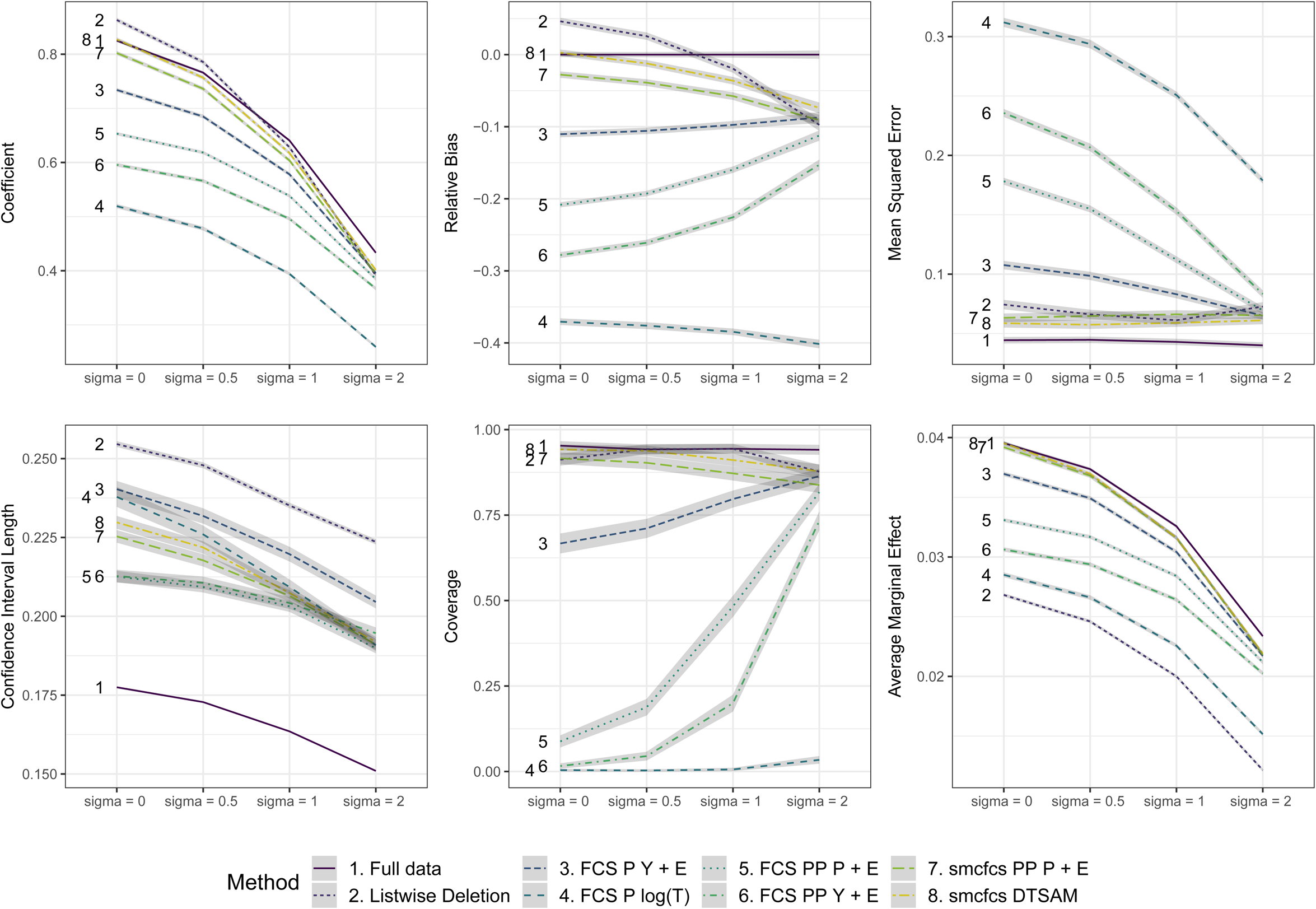
Figure 1 displays the performance measures for the estimates of $β_{1}$ . The population parameters (i.e., the true values), used for the calculation of the performance estimates, were estimated from the created population with N=1,000,000. The bias is displayed for no unobserved heterogeneity and increasing unobserved heterogeneity with frailty term variance $σ^{2} = 0.25$ , $σ^{2} = 1$ , and $σ^{2} = 4$ , respectively.

Figure 1.

Performance measures for coefficient $β_{1}$ (for $X_{1}$ ). Grey areas 95% confidence interval for performance measures. One thousand Monte Carlo (MC) repetitions with 2,000 simulated persons per simulation. All cells apart from the diagonal in the correlation matrix of $X_{1}, \dots, X_{5}$ are 0.1. Censoring of time after 15 time units. $α$ -parameters for time indicators are $(- 4, \dots, - 1)$ and $β = (0.8, 2.2, - 0.5, 0.3, - 1.4)$ for covariates $X_{1}, \dots, X_{5}$ . $X_{1}$ , $X_{2}$ and $X_{3}$ are missing depending on $X_{4}$ , $X_{5}$ , $Y$ with $β_{m i s s}$ =(2,2,2). PP format: person-period format; P format: person-oriented format; FCS: fully conditional specification; SMC-FCS: substantive-model compatible-fully conditional specification. See also the online Appendix Tables A3–A6.

We concentrate first on the imputation methods under no unobserved heterogeneity on the left. The assumption of proportional odds is thus fulfilled for the analysis model with full data and the model is correctly specified. As LD overestimates the true coefficient, and the CI length and MSE are about 50% higher than that of the full data, there is room for improvement in terms of bias and efficiency. Turning to the different imputation methods and their performance, we notice profound differences. We register the highest bias for the imputation approach FCS P $l o g (T)$ . As in the case of the Cox model, this approach is completely inadequate (Beesley et al., 2016: 4711). The second and third-to-worst approaches are the two FCS approaches in PP format (5. FCS PP $P + E$ and 6. FCS PP $Y + E$ ) with the current period and the censored survival time, respectively, included in the imputation models.

The FCS approach in P format using the information from the (censored) survival time and the event indicator (3. FCS P $Y + E$ ) is also not satisfying, bias is still high, coverage low and the MSE is higher than after LD. This leaves us with the two SMC-FCS approaches (7. SMC-FCS PP $Y + E$ and 8. SMC-FCS DTSAM). Both methods and especially the new SMC-FCS DTSAM approach perform better than LD in terms of bias and MSE as well as the CI length and the corresponding coverage for no unobserved individual heterogeneity/frailty. Plus, the AME estimate shows very little bias for the two SMC-FCS methods in comparison to all other approaches which all lead to underestimation.

We now move on to add unobserved heterogeneity to the data-generating process (variance of the frailty term $σ^{2} = 0.25$ or $σ^{2} = 1$ , $σ^{2} = 4$ ). Since the DTSAM model thus omits the frailty variables—a very common misspecification which can be hard to address (Allison, 1982)—we explore the performance of imputation approaches under this condition. With increasing heterogeneity, the logistic regression coefficients are drawn towards zero by unobserved heterogeneity (Mood, 2009). The SMC-FCS approaches do not perform as well as with no frailties present with high unobserved heterogeneity, but still better than most other approaches. Whereas some of the performance measures for FCS approaches perform as well as the SMC-FCS approaches in the case of high heterogeneity regarding relative bias or MSE, they do not perform better than the SMC-FCS approaches in regard to the estimation of AMEs. As AMEs are often used in the comparison of different DTSAM models (e.g., Wagner et al., 2019: 84), we also include them in our performance evaluation.

From all that we have seen so far, the new SMC-FCS DTSAM approach outperforms or performs at least as well as all other imputation models and is therefore recommended. The currently most common approach, LD, leads to high-efficiency losses and possibly high bias, and should therefore be avoided. The amount of heterogeneity that can be modeled in a DTSAM will vary strongly with available variables, but SMC-FCS DTSAM performs comparatively well.

Further Simulation Results

This article focuses on the effect of unobserved heterogeneity on the results of different imputation strategies and presents the new SMC-FCS DTSAM approach. It is also important to check whether the new method is suited to a broader range of circumstances. Therefore, we also conducted additional simulations, varying other factors such as the percentage of observations missing, the data-generating model, the amount of censoring, the correlation of covariates, and the amount of missingness in the online Appendix Figures A3–A7. Briefly summarizing the results of the five additional simulations, we notice that SMC-FCS DTSAM also performs very well under all other simulated scenarios. Several other solutions such as the two FCS imputation approaches in PP are also suited if there is no unobserved heterogeneity. FCS in-person format with $\log (T)$ shows inadequate performance in almost all circumstances. Summing up, SMC-FCS DTSAM is the method that showed good performance in all cases and is therefore recommended.

An Applied Example with the German Family Panel Pairfam

To provide an applied example under real-world data conditions, we now conduct an example analysis from the field of relationship and family research using data from the German Family Panel project called pairfam (Brüderl et al., 2017).

The 2008-launched pairfam panel (“Panel Analysis of Intimate Relationships and Family Dynamics”) is a longitudinal study for research on relationships and families in Germany. The data are collected from a nationwide random sample of the three birth cohorts 1971–1973, 1981–1983, 1991–1993, and their partners, parents, and children. For our real-world example, we used data from the data set biopart, which includes prospective and retrospective information on the anchor’s relationships, including relationships, cohabitation, and marriage history. We used the data set 8.0.0 (Brüderl et al., 2017), which includes updated information from the survey waves 1–9 (for more details on the panel, see Huinink et al., 2011).

We use a simple substantive model from the field of relationship stability research. Note that our goal here is not to estimate any causal models but rather to explore how our imputation approaches fare with a real data set. Let us assume that we are interested in the relationship between the probability that a couple $i$ splits up and several time-invariant independent variables.

We first include six indicators 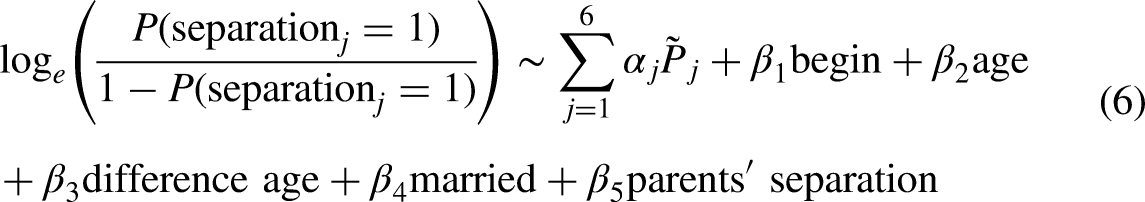${\tilde{P}}_{j}$ with $j = {1, 2, \dots, 6}$ , for grouped periods, $1, 2, \dots, 5$ each representing five years of a relationship and 6 representing all years after 25 years of a relationship. These variables include the time point at which the relationship started (begin in years since 1900), the age in years when the anchor person began the relationship (age), the difference in ages of the two relationship partners (difference age), an indicator for whether the partners are married (married) and an indicator for whether the parents separated during the anchor’s childhood (parents’ separation).³

\begin{aligned} \log_{e} (\frac{P ({separation}_{j} = 1)}{1 - P ({separation}_{j} = 1)}) \sim \sum_{j = 1}^{6} α_{j} {\tilde{P}}_{j} + β_{1} begin + β_{2} age \\ + β_{3} difference age + β_{4} married + β_{5} parent s^{'} separation \end{aligned}

(6)

We reduce the data set to the fully observed first-reported relationships of all anchors. This leaves us with a sample of 2,173 relationships. Transforming the data set to the relationship-year format leads to 26,554 rows (i.e., observed periods). For our data set with missing data, we deleted 30% of the observations for three of the variables, namely, age, begin, and parents’ separation. The values are missing at random (MAR)—that is, missingness depends on the censored time to survival, whether the relationship failed, whether the partners are married to each other, and the two respective other variables with missing data. We then impute the missing values using the same approaches we already tested in the simulations using normal models for the two continuous covariates and a logistic model for the binary one.

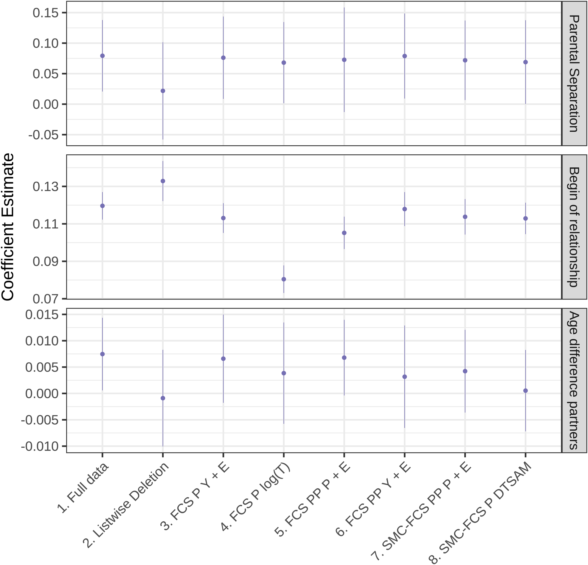
Examining the results in Figure 2, we notice that after LD, the coefficient estimate for begin has a higher variance. We also see that after imputing with our various approaches, the imputation approach FCS P $l o g (T)$ (4) again performs differently and worse than the other imputation approaches; the coefficient of begin is way off; the 95% confidence interval does not even come close to the interval of the full data. There are few differences between the other imputation approaches for this real-life data set, but we want to mention that the new SMC-FCS DTSAM approach performs adequately in this real-world setting, as was also the case in the simulation.

Figure 2.

Selected estimated coefficients for a DTSAM of the separation of the first fully observed reported relationships. German Family Panel (pairfam) Data Set 8.0.0 (Brüderl et al., 2017) with MAR data introduced by the authors. For the specification of the DTSAM see equation (6). DTSAM: discrete-time survival analysis model; MAR: missing at random.

In sum, the findings resemble those found in the simulations. They show (1) that some imputation approaches—for example, treating the time-to-event variable as partly unobserved—are not advisable; (2) that imputing in PP format with FCS cannot be recommended; and (3) that SMC-FCS with a compatible imputation model performs adequately.

Discussion

Results

Like many other types of data analysis, the analysis of discrete-time survival data is often challenged by missing data in one or more covariates. Negative consequences of such missing data include efficiency losses and bias. A popular approach to circumventing these consequences is MI. However, in MI, it is crucial to include outcome information in the model for imputing partially observed covariates. Unfortunately, this is not straightforward in the case of discrete-time survival data because (1) we usually have a partially observed (left- or right-censored or both) outcome; (2) we do not have just one outcome variable, but two (i.e., event and time-to-event); and (3) we have to decide whether to impute while the data set is still in the P format or after conversion to PP format, especially if we are looking at time-invariant variables.

In this article, we have tested different approaches for imputing missing covariates in the discrete-time survival analysis model (DTSAM) setting. For this purpose, we performed four simulations that differed in the amount of unobserved heterogeneity. Some of the investigated methods are from the literature on the imputation of time-constant variables for the Cox model (van Buuren, Boshuizen, and Knook, 1999; White and Royston, 2009; Clark and Altman, 2003; Keogh and Morris, 2018; Beesley et al., 2016). We also present a new SMC-FCS approach implemented as smcfcs.dtsam in the R package smcfcs that allows time-invariant imputations and at the same time uses a compatible imputation model. We also provided an applied example using pairfam data (Brüderl et al., 2017).

Our findings lead us to agree with Beesley et al. (2016) that treating censored survival times as partially unobserved and imputing other covariates depending on the multiply imputed missing survival times yields unsatisfying results in all cases when one is using existing imputation methods for imputing $T$ , and these are not be using the correct model. Whereas Beesley et al. (2016) observed this for the Cox (cure) model, we have confirmed it for discrete-time survival analyses.

Furthermore, the performance of imputation methods in PP format with FCS is disappointing. Apart from the inherent incoherence between the imputed values for different times in the same person, coverage and relative bias are unsatisfying. The new SMC-FCS DTSAM approach using a compatible imputation model performs best in our simulations with and without unobserved heterogeneity and is therefore strongly recommended.

Limitations and Future Research

An open question regarding imputation within the context of DTSAM models is how to best impute missing values for time-varying covariates (for a general overview of joint models of longitudinal and survival data, see Papageorgiou et al. 2019). Imputing with standard FCS or SMC-FCS approaches in PP format is possible but will not reflect correlations over time within individuals of the values of the time-varying variables. Research to confirm the adequate performance of simple approximations or the development of new methods in the case of time-varying covariates has yet to be undertaken.

Another open question is how to deal with the time-varying effects of time-invariant and time-varying covariates. Keogh and Morris (2018) have shown that a variation of the SMC-FCS approach also performs sufficiently well in the case of time-varying covariates. Again, an evaluation for discrete-time survival models has not yet been conducted.

Conclusions

We recommend using the newly developed SMC-FCS DTSAM approach that allows imputations that are time-invariant (do not differ between periods for a unit) and at the same time are imputed from imputation models which are compatible with the DTSAM specified by the user. The general SMC-FCS approach has already shown excellent performance in the case of included quadratic covariates and interaction effects in linear and logistic regression as well as for the imputation of covariates in Cox (cure) regressions (Bartlett et al., 2015b; Bartlett and Taylor, 2016; Beesley et al., 2016; Keogh and Morris, 2018). The new SMC-FCS DTSAM approach performed at least as well as—and usually better than—the other SMC-FCS approaches we explored in this article.

Footnotes

Author’s Note

The code for this article is available at the Open Science Framework: https://osf.io/txvey/?view˙only=04116ea9a8934b5aaf9a41059c254213. It is divided into code for the main part of the article and code for the additional simulations in the online Appendix. The data for the applied example is available as a Scientific Use File on the pairfam website: https://www.pairfam.de/en/data/. The newly developed smcfcs-dtsam method is also documented on CRAN: .

Declaration of Conflicting Interests

The author(s) declared no potential conflicts of interest with respect to the research, authorship, and/or publication of this article.

Funding

The author(s) disclosed receipt of the following financial support for the research, authorship, and/or publication of this article: Funded partially by the Deutsche Forschungsgemeinschaft (DFG) under project number 316901171.

ORCID iDs

Anna-Carolina Haensch

Jonathan Bartlett

Bernd Weiß

Notes

Author Biographies

Anna-Carolina Haensch is a postdoctoral research at the Institute of Statistics at the LMU Munich in Germany. Her research interests include developing multiple imputation and synthetic data approaches.

Jonathan Bartlett is a professor in Medical Statistics at the London School of Hygiene & Tropical Medicine. His research involves developing methods and software for handling missing data, measurement error, and more recently, causal inference, particularly when applied to randomised trials.

Bernd Weiß is team leader of the GESIS Panel and deputy head of the Department Survey Design and Methodology at GESIS Leibniz Institute for the Social Sciences in Mannheim, Germany.

References

Aalen

Odd

. 1994. “Effects of Frailty in Survival Analysis.” Statistical Methods in Medical Research 3:227-243.

Allison

Paul

. 1982. “Discrete-Time Methods for the Analysis of Event Histories.” Sociological Methodology 13:61-98.

Allison

Paul

. 2000. “Multiple Imputation for Missing Data: A Cautionary Tale.” Sociological Methods & Research 28:301-309.

Arránz Becker

Oliver

Lois

Daniel

. 2010. “Unterschiede im Heiratsverhalten Westdeutscher, Ostdeutscher und Mobiler Frauen: Zur Bedeutung von Transformationsfolgen und Soziokulturellen Orientierungen.” Soziale Welt 61:5-26.

Arranz Becker

Oliver

Lois

Daniel

. 2013. “Competing Pleasures? The Impact of Leisure Time Use on the Transition to Parenthood.” Journal of Family Issues 34:661-688.

Barber

Jennifer

. 2001. “Ideational Influences on the Transition to Parenthood: Attitudes Toward Childbearing and Competing Alternatives.” Social Psychology Quarterly 64:101-127.

Bartlett

Jonathan

Keogh

Ruth

. 2019. smcfcs: Multiple Imputation of Covariates by Substantive Model Compatible Fully Conditional Specification. R Package Version 1.4.0.

Bartlett

Jonathan W.

Harel

Ofer

Carpenter

James R.

. 2015a. “Asymptotically Unbiased Estimation of Exposure Odds Ratios in Complete Records Logistic Regression.” American Journal of Epidemiology 182:730-736.

Bartlett

Jonathan W.

Seaman

Shaun R.

White

Ian R.

Carpenter

James R.

. 2015b. “Multiple Imputation of Covariates by Fully Conditional Specification: Accommodating the Substantive Model.” Statistical Methods in Medical Research 24:462-487.

10.

Bartlett

Jonathan W.

Taylor

Jeremy M. G.

2016. “Missing Covariates in Competing Risks Analysis.” Biostatistics (Oxford, England) 17:751-763.

11.

Beesley

Lauren

Bartlett

Jonathan

Wolf

Gregory

Taylor

Jeremy

. 2016. “Multiple Imputation of Missing Covariates for the Cox Proportional Hazards Cure Model.” Statistics in Medicine 35:4701-4717.

12.

Böttcher

Karin

. 2006. “Scheidung in Ost- und Westdeutschland.” KZfSS Kölner Zeitschrift für Soziologie und Sozialpsychologie 58:592-616.

13.

Brüderl

Josef

Hank

Karsten

Huinink

Johannes

Nauck

Bernhard

Neyer

Franz J.

Walper

Sabine

Alt

Philipp

Borschel

Elisabeth

Buhr

Petra

Castiglioni

Laura

Friedrich

Stefan

Finn

Christine

Garrett

Madison

Hajek

Kristin

Herzig

Michel

Huyer-May

Bernadette

Lenke

Ruediger

Müller

Bettina

Peter

Timo

Schmiedeberg

Claudia

Schütze

Philipp

Schumann

Nina

Thönnissen

Carolin

Wetzel

Martin

Wilhelm

Barbara

. 2017. “The German Family Panel (pairfam).” Technical Report ZA5678 Data file Version 8.0.0, GESIS Data Archive, Cologne.

14.

Carpenter

James

Kenward

Michael

. 2013. Multiple Imputation and Its Application. Hoboken: Wiley.

15.

Clark

Taane

Altman

Douglas

. 2003. “Developing a Prognostic Model in the Presence of Missing Data: An Ovarian Cancer Case Study.” Journal of Clinical Epidemiology 56:28-37.

16.

Cooke

Lynn Prince

. 2006. “Doing Gender in Context: Household Bargaining and Risk of Divorce in Germany and the United States.” American Journal of Sociology 112:442-472.

17.

Cooper

Maria

Loukas

Alexandra

Case

Kathleen R.

Marti

C. Nathan

Perry

Cheryl L.

2018. “A Longitudinal Study of Risk Perceptions and E-cigarette Initiation Among College Students: Interactions with Smoking Status.” Drug and Alcohol Dependence 186:257-263.

18.

David

Cox

. 1972. “Regression Models and Life-Tables.” Journal of the Royal Statistical Society. Series B (Methodological) 34:187-220.

19.

Erler

Nicole S.

Rizopoulos

Dimitris

Lesaffre

Emmanuel M. E. H.

. 2021. “JointAI: Joint Analysis and Imputation of Incomplete Data in R.” Journal of Statistical Software 100(20):1-56. doi: 10.18637/jss.v100.i20

20.

Fay

Robert E

. 1992. “When Are Inferences from Multiple Imputation Valid?” In Proceedings of the Survey Research Methods Section of the American Statistical Association, volume 81, 227-232.

21.

Hughes

Rachael

Heron

Jon

Sterne

Jonathan

Tilling

Kate

. 2019. “Accounting for Missing Data in Statistical Analyses: Multiple Imputation is Not Always the Answer.” International Journal of Epidemiology 48:1294-1304.

22.

Huinink

Johannes

Brüderl

Josef

Nauck

Bernhard

Walper

Sabine

Castiglioni

Laura

Feldhaus

Michael

. 2011. “Panel Analysis of Intimate Relationships and Family Dynamics (pairfam): Conceptual Framework and Design.” Zeitschrift für Familienforschung 23:77-101.

23.

Kenward

Michael G.

Carpenter

James

. 2007. “Multiple Imputation: Current Perspectives.” Statistical Methods in Medical Research 16:199-218.

24.

Keogh

Ruth

Morris

Tim

. 2018. “Multiple Imputation in Cox Regression when there are Time-Varying Effects of Covariates.” Statistics in Medicine 37:3661-3678.

25.

Klein

Thomas

Kopp

Johannes

Rapp

Ingmar

. 2013. “Metaanalyse Mit Originaldaten. Ein Vorschlag zur Forschungssynthese in der Soziologie.” Zeitschrift für Soziologie 42:222-238.

26.

Kleinbaum

David G.

Klein

Mitchel

. 2012. Survival Analysis. A Self-Learning Text. 3rd ed. New York: Springer.

27.

Little

Roderick

. 2019. Statistical Analysis with Missing Data. Hoboken, NJ: Wiley.

28.

Little

Roderick

Rubin

D. B.

2002. Statistical Analysis with Missing Data. Hoboken: Wiley.

29.

Manning

Wendy D.

Brown

Susan L.

Stykes

J. Bart

. 2016. “Same-Sex and Different-Sex Cohabiting Couple Relationship Stability.” Demography 53:937-953.

30.

McGilchrist

C. A.

Aisbett

C. W.

1991. “Regression with Frailty in Survival Analysis.” Biometrics 47:461-466.

31.

Meng

Xiao-Li

. 1994. “Multiple-Imputation Inferences with Uncongenial Sources of Input.” Statistical Science 9:538-558.

32.

Mood

Carina

. 2009. “Logistic Regression: Why We Cannot Do What We Think We Can Do, and What We Can Do About It.” European Sociological Review 26:67-82.

33.

Murad

Havi

Dankner

Rachel

Berlin

Alla

Olmer

Liraz

Freedman

Laurence S

. 2019. “Imputing Missing Time-Dependent Covariate Values for the Discrete Time Cox Model.” Statistical Methods in Medical Research 29(8):2074-2086.

34.

Nomaguchi

Kei M.

. 2006. “Time of One’s Own. Employment, Leisure, and Delayed Transition to Motherhood in Japan.” Journal of Family Issues 27:1668-1700.

35.

Nur

Ula

Shack

Lorraine

Rachet

Bernard

Carpenter

James

Coleman

Michel

. 2009. “Modelling Relative Survival in the Presence of Incomplete Data: A Tutorial.” International Journal of Epidemiology 39:118-128.

36.

Papageorgiou

Grigorios

Mauff

Katya

Tomer

Anirudh

Rizopoulos

Dimitris

. 2019. “An Overview of Joint Modeling of Time-to-Event and Longitudinal Outcomes.” Annual Review of Statistics and Its Application 6:223-240.

37.

R Core Team. 2019. R: A Language and Environment for Statistical Computing. Vienna, Austria: R Foundation for Statistical Computing.

38.

Rubin

D. B.

1987. Multiple Imputation for Nonresponse in Surveys. Hoboken: Wiley.

39.

Rubin

Donald B.

1996. “Multiple Imputation After 18+ Years.” Journal of the American Statistical Association 91:473-489.

40.

Schafer

Joe L.

1997. Analysis of Incomplete Multivariate Data. London: Chapman and Hall.

41.

Schoen

Robert

Astone

NanMarie

Rothert

Kendra

Standish

Nicola J.

Kim

Young J.

2002. “Women’s Employment, Marital Happiness, and Divorce.” Social Forces 81:643-662.

42.

Singer

Judith D.

Willett

John B.

1993. “It’s About Time: Using Discrete-Time Survival Analysis to Study Duration and the Timing of Events.” Journal of Educational Statistics 18:155-195.

43.

Singer

Judith D.

Willett

John B.

2003. Applied Longitudinal Data Analysis. New York, New York, USA: Oxford University Press.

44.

Stoddard

Sarah A.

Veliz

Philip

. 2019. “Summer School, School Disengagement, and Substance Use During Adolescence.” American Journal of Preventive Medicine 57:11-15.

45.

van Buuren

Stef

. 2007. “Multiple Imputation of Discrete and Continuous Data by Fully Conditional Specification.” Statistical Methods in Medical Research 16:219-242.

46.

van Buuren

Stef

Boshuizen

Hendriek C.

Knook

D. L.

. 1999. “Multiple Imputation of Missing Blood Pressure Covariates in Survival Analysis.” Statistics in Medicine 18:681-694.

47.

Vaupel

James

Manton

Kenneth

Stallard

Eric

. 1979. “The Impact of Heterogeneity in Individual Frailty on the Dynamics of Mortality.” Demography 16:439-454.

48.

Wagner

Michael

Mulder

Clara H.

Weiss

Bernd

Krapf

Sandra

. 2019. “The Transition From Living Apart Together to a Coresidential Partnership.” Advances in Life Course Research 39:77-86.

49.

White

Ian R.

Royston

Patrick

. 2009. “Imputing Missing Covariate Values for the Cox Model.” Statistics in Medicine 28:1982-1998.

50.

White

Ian R.

Royston

Patrick

Wood

Angela M.

2011. “Multiple Imputation Using Chained Equations: Issues and Guidance for Practice.” Statistics in Medicine 30:377-399.

51.

Xue

Xiaonan

Brookmeyer

Ron

. 1996. “Bivariate Frailty Model for the Analysis of Multivariate Survival Time.” Lifetime Data Analysis 2:277-289.

Multiple imputation of partially observed covariates in discrete-time survival analysis

Abstract

Keywords

Introduction

Discrete-Time Survival Analysis Model

The Model

The Data: Transformations and the Person-Period Format

Implications of Missing Data for Discrete-Time Survival Analysis

Multiple Imputation

MI in General

Handling Missing Covariates Values in Case of a DTSAM as a Substantive Model

FCS with Data in P Format

FCS with Data in PP Format

SMC-FCS with Data in PP Format

A New SMC-FCS Approach: SMC-FCS DTSAM

Simulation Study

Data-Generating Mechanisms

Missingness

Methods Compared and Performance Measures

Simulation Results

Further Simulation Results

An Applied Example with the German Family Panel Pairfam

Discussion

Results

Limitations and Future Research

Conclusions

Footnotes

Author’s Note

Declaration of Conflicting Interests

Funding

ORCID iDs

Notes

Author Biographies

References