A Rolling Panel Model of Cohort,Period,and Aging Effects for the Analysis of the General Social Survey

Abstract

The linear dependence of age, period, and birth cohort is a challenge for the analysis of social change. With either repeated cross-sectional data or conventional panel data, raw change cannot be decomposed into over-time differences that are attributable to the effects of common experiences of alternative birth cohorts, features of the periods under observation, and the cumulation of lifecourse aging. This article proposes a rolling panel model for cohort, period, and aging effects, suggested by and tuned to the treble panel data collected for the General Social Survey from 2006 through 2014. While the model does not offer a general solution for the identification of the classical age-period-cohort accounting model, it yields warranted interpretations under plausible assumptions that are reasonable for many outcomes of interest. In particular, if aging effects can be assumed to be invariant over the course of an observation interval, and if separate panel samples of the full age distribution overlap within the same observation interval, then period and aging effects can be parameterized and interpreted separately, adjusted for cohort differences that pulse through the same observation interval. The estimated cohort effects during the observation interval are then interpretable as effects during the observation interval of entangled period and cumulated aging differences from before the observation interval.

Introduction

When raw changes in attitudes and opinions accelerate rapidly, or when they are abrupt and pronounced, researchers naturally conclude that social and institutional events, occurring during the same time period, are at least partly responsible. For the interval considered in this article, the General Social Survey (GSS) provides several examples. Support for the legalization of marijuana and acceptance of same-sex marriage both increased by approximately 20% from 2006 to 2014 alongside precedent-setting court decisions and legislative changes. ¹ Support for additional national spending “to improve and protect the nation's health” increased slightly between 2006 and 2008 while several presidential election campaigns promoted healthcare reform. Then, after the passage of the Affordable Care Act in 2010, support for additional health spending fell by 17%, and it did not rebound substantially in either 2012 or 2014. ² Finally, the Great Recession pushed down self-evaluations of whether one's financial situation was improving from 40% in 2006 to a low of only 25% in 2010 – the lowest level recorded by the GSS since its inception in 1972. As the economy improved, these self-evaluations increased to 36% by 2014, completing a U-turn that tracked the overall economy and its slow recovery from the recession.

Claims about the importance of events in recent periods, however, must contend with the possibility that events from prior periods are also responsible for at least part of an observed change. Any past “experiential chasm between cohorts” (Ryder 1965:850) can generate a change observed in a later time period because of the cohort replacement that accompanies population change. Moreover, when any such consequential events from prior periods occur, the resulting cohort differentiation occurs at particular ages in the history of each birth cohort. The analyst must then confront the age, period, cohort (APC) identification challenge, which for most conventional data structures is undermined by linear dependence that restricts the observed variation. Each cohort's observed age is exactly equal to the cohort's year of birth plus the number of periods, enumerated by years, that each cohort has lived through.

In this article, we analyze the rolling panel data collected for the GSS from 2006 to 2014. ³ Our primary goal is to propose an empirical model, resting on clear substantive assumptions, that can be used to investigate how cohort, period, and aging effects generate change during an explicit observation interval. In the remainder of this introductory section, we offer an orientation to the APC literature, identifying the components that we will build upon. We also provide an introduction to some of the conceptual grounding we will use, which differs to a modest degree from the APC literature that considers only the analysis of repeated cross-sectional data from the classical accounting-model tradition. This material also motivates our secondary goal for the article, which is to use the GSS panel data to explain some limitations that are common in the extant APC literature: inattention to the underlying open-cohort structure of repeated cross-sectional data as well as motivations of estimands that do not specify how cohort effects are related to past period and aging effects.

Departure Point from the APC Literature

The APC literature is extensive, and much insight can be gained by considering how overview accounts have evolved from early pieces that established the conceptual foundations through the more recent work that debates identification claims for more recent modeling approaches – from pieces such as Ryder (1965), Glenn (1977), and Hobcraft, Menken, and Preston (1982), to Firebaugh (1997) and Glenn (2005), and then O’Brien (2017) and Fosse and Winship (2019). Since 2000, many pieces in the APC literature have debated the value of new approaches that impose novel constraints on the data in attempts to break the modeling impasse articulated clearly by the 1980s (see Yang and Land 2013 for many of these approaches). On balance, and after much critique, it now appears that these new models do not provide as much insight as desired (see Bell and Jones 2018; Fosse and Winship 2018; Luo 2013; Luo and Hodges 2015, 2020a; O’Brien 2015, 2017).

Mindful of these debates, and lessons from them, we do not attempt to develop a solution to the classical APC challenge associated with the accounting model of Mason et al. (1973). Our contribution is to return to the idea that repeated individual-level measurement is a design advantage that, when paired with reasonable assumptions, may be able to deliver some warranted conclusions. The most developed early precursor of our approach is Duncan and Stenbeck (1988), but the idea of using some type of within-respondent variation to estimate lifecourse aging effects within an APC setup had occurred to others earlier (Glenn 1974, 1977, Hout and Knoke 1975, and presumably many others). Regardless of origin, the design advantage of repeated measurement has percolated in the literature, including in substantive research that is not directly connected to the APC literature (e.g., Armenia and Troia 2017, Tilley and Evans 2014, and Stoker and Jennings 2008).

Partly because of the variation that our rolling panel data provides, our approach suggests model interpretations that align with recent work on alternative characterizations of cohort effects, such as Keyes et al. (2010), Luo and Hodges (2020b), and Schulhofer-Wohl and Yang (2016). The additivity constraints of the multiple-classification, accounting model of Mason et al. (1973) and Fienberg and Mason (1979) are too rigid for the range of explanatory puzzles that can be generated by age, period, and cohort effects. A potentially more productive starting point is to stipulate, as a first principle, that cohort effects arise precisely from the interaction of period and age effects. This position has been recognized within the APC literature all along (see Ryder 1965:847-48), but subsequent work that has been pursued under the additivity constraints of the accounting model has obscured it.

Conceptual Grounding for Our Approach

Because we will offer results using rolling panel data, we must adopt an interpretive framework that captures the details that our panel data require us to consider and allow us to model. We offer in this section a brief introduction, hoping to head off misunderstandings that might otherwise arise, especially for readers who are familiar only with the accounting-model tradition of APC analysis.

First, we use the term observation interval to refer to the range of the period variation selected for analysis, which for our models will be the interval from 2006 to 2014 when the rolling panel data of the GSS are available. As a result, like all APC analyses, the period effects we model directly are only a subset of the periods that our respondents lived through.

Second, we accept the standard position that cohort differences generate raw change through cohort replacement. However, we conceive of the cohort differences that generate raw change somewhat differently than researchers who analyze only repeated cross-sectional data while adhering to the additivity constraints of the accounting model. For the type of attitude-change research typically pursued with data sources such as the GSS, the classic example is the set of differences between those who entered adulthood during the Great Depression and New Deal and those who were born in the baby boom that followed World War II. Individuals who lived through the Great Depression experienced a shared period of economic distress and then government interventionism that boomers born after 1946 did not. In addition, and in part because of increased affluence, many more boomers were able to delay marriage and labor-force entry in order to take advantage of evolving opportunities to acquire postsecondary education. When boomers entered into adulthood, these interactive period and aging differences between the 1930s and the 1960s began to generate population-averaged raw change in attitudes and opinions through cohort replacement from the 1970s onward (see Knoke and Hout 1974; Alwin, Cohen, and Newcomb 1991). For our rolling panel data model, we will take the position that the effects of cohort differences during our explicit observation interval are best thought of as effects during the observation interval that are attributable to entangled prior period and cumulated age differences passing through the observation interval. ⁴

As an implication of these positions, and with reference to the goals of the existing APC literature based on the accounting model, we will pursue a type of identification for cohort, period, and aging effects that could be considered “conditional.” In particular, we will attempt to estimate period and aging effects for differences that occur during an observation interval, conditional on estimated cohort effects. Accordingly, we will not present in this article a solution to the APC identification problem in the form articulated by Mason et al. (1973) and that is the primary focus of the work summarized in review pieces such as Fosse and Winship (2019). We do not claim that we can separate out from our estimated cohort effects the components of those effects that are attributable to cumulated age differences at the point of entry into the observation interval. For this reason, we do not challenge the claim of Glenn (1976) that the search for a solution to the APC challenge defined by the accounting model is a “futile quest.” ⁵

In the next section, we introduce details of the data and measures we analyze. We then provide a series of estimated models – first, for a baseline APC analysis and, second, for our proposed rolling panel data model. After demonstrating the range of substantive interpretations that the panel data model can generate, we then detail and discuss three specific identification assumptions that warrant the substantive interpretations.

Data and Methods

From 2006 to 2014, the GSS was fielded as both a repeated cross-sectional survey of the adult population and as a rolling panel. Cross-sectional samples were drawn biennially from 2006 to 2014, and the three cross-sectional samples drawn in 2006, 2008, and 2010 were reinterviewed two and four years later. This design preserved the repeated cross-sectional structure of the GSS while also yielding a “treble panel” – three overlapping panels of three waves each (see Smith and Schapiro 2017; see also Hout and Hastings 2016 and Morgan and Lee 2020).

In this article, we analyze the GSS data in the two distinct configurations that this design allows. First, we pool and then analyze the five cross-sectional samples drawn in 2006, 2008, 2010, 2012, and 2014 (see Smith, Davern, Freese, and Morgan 2019). For this traditional setup, we ignore the repeated measures available in the panel follow-up waves. Second, we pool and analyze all components of the treble panel. In this second configuration, we append the three panels, using all nine sets of observations, and we adjust for panel attrition with the weights developed by Morgan and Lee (2020). The structure of the rolling panel data is depicted in Figure 1.

Figure 1.

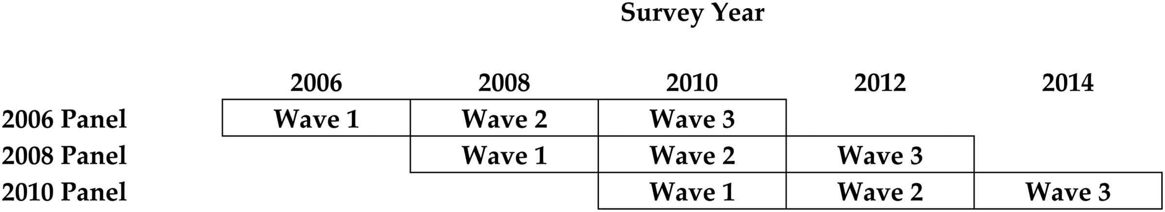
The rolling panel design of the GSS from 2006 to 2014.

In both configurations, we analyze pooled datasets with observations collected biennially from 2006 to 2014. As noted below in the results, and as discussed in more detail in the appendix, the two configurations differ subtly in the implied target population for analysis.

Measures

For traditional APC measures, we use age, year of observation, and year of birth. We also use panel wave to index within-respondent change, and this variation can be used to estimate aging effects when cohort and period effects are fit simultaneously.

For outcomes, we use the seven items presented in Table 1. Collectively, these outcomes represent patterns of change for a small subset of the GSS core measures from 1972 to 2018 (see Hout 2020; Marsden, Smith, and Hout 2020). Five were selected because the literature suggests that they changed in particularly interesting ways between 2006 and 2014: support for the legalization of marijuana, two measures for support of same-sex relations, self-assessed financial situation, and support for increases in health spending.

Table 1.

Selected Outcome Variables from the Core Items of the GSS.

GSS Variable	Question Wording	Response Categories	Coding for Analysis
Support for legalization of marijuana (GRASS)	Do you think the use of marijuana should be made legal, or not?	Should Should not No opinion	1 for should, 0 for should not, and missing for no opinion
Support for the position that same-sex sexual relations are not wrong at all (HOMOSEX)	What about sexual relations between two adults of the same sex – do you think it is always wrong, almost always wrong, wrong only sometimes, or not wrong at all?	Always wrong Almost always wrong Wrong only sometimes Not wrong at all Don't know	1 for not wrong at all, 0 for all else, and missing for don't know
Support for same-sex marriage (MARHOMO)	Do you agree or disagree with the following statement: Homosexual couples have the right to marry one another	Strongly agree Agree Neither agree nor disagree Disagree Strongly disagree	1 for strongly agree or agree, 0 for all else
Financial situation has been getting better (FINALTER)	During the last few years, has your financial situation been getting better, getting worse, or has it stayed the same?	Getting better Getting worse Stayed the same Don't know	1 for getting better, 0 for all else, and missing for don't know
Need more spending on health (NATHEAL)	First I would like to talk with you about some things people think about today. We are faced with many problems in this country, none of which can be solved easily or inexpensively. I’m going to name some of these problems, and for each one I’d like you to tell me whether you think we’re spending too much money on it, too little money, or about the right amount. Improving and protecting the nation's health (1/2 sample), Health (1/2 sample)	Too much Too little About right Don't know	1 for too little, 0 for all else, and missing for don't know
Need more spending on education (NATEDUC)	Improving the nation's education system (1/2 sample), Education (1/2 sample)	Too much Too little About right Don't know	1 for too little, 0 for all else, and missing for don't know
Vocabulary knowledge (WORDSUM)	A ten-item vocabulary test	1 correct and 3 incorrect definitions for each word	0 to 10 correct

Notes: The GSS mnemonic variable names are in parentheses in column 1.

For comparison, we selected two measures that the literature suggests present much simpler patterns of over-time change. First, we selected support for spending increases in education, given that it is parallel in structure to the more dynamic measure of support for health spending and that it has been used in past research to examine social change and APC dynamics (see Firebaugh 1997, 2008; Plutzer and Berkman 2005). Second, we selected the test of vocabulary knowledge. This outcome has been examined extensively in the APC literature, with both a substantive orientation (from Alwin 1991 and Glenn 1994 through critiques reevaluated by Alwin and Pacheco 2012) and as a demonstration example in the methodological literature (e.g., Yang and Land 2006; Fosse and Winship 2019). As will become clear below, we selected the vocabulary test because it shows how the proposed model does not suggest change where past scholars have made reasonable claims that change does not exist. Thus, the vocabulary test is a type of conceptual placebo that should allay concerns that the model produces perplexing results.

We dichotomize the attitude responses, using the coding shown in the final column of Table 1, and we then scale the attitudes so that the resulting coefficients can be given percent interpretations (to conform with conventions in public-opinion research). We leave the vocabulary test in its raw scale (0 to 10).

Model Estimation

We use least-squares regression for model estimation. None of the results we offer are driven meaningfully by this choice. We show in the appendix that logit models generate results that are only trivially different.

Baseline Results for Comparison from Repeated Cross-Sections

We first explain the core APC identification challenge for measured over-time change, using the example of attitudes toward the legalization of marijuana from 2006 through 2014. We also use these results to motivate a discussion of a secondary limitation of this type of APC model – an inherently “open cohort” structure – that a panel data approach can address more satisfactorily.

A Standard Cohort Analysis of Attitude Change

With support for the legalization of marijuana as the outcome, Table 2 presents four models for the 7,142 respondents in the repeated cross-sectional data. The first three models are specified as

$$y_i=\hat{\alpha }+{\hat{\beta }}_{c}birth\mathrm{\_}yea{r}_i+{\epsilon }_i$$

(1)

$$y_i=\hat{\alpha }+{\hat{\beta }}_{p}year\mathrm{\_}of\mathrm{\_}measuremen{t}_i+{\epsilon }_i$$

(2)

$$y_i=\hat{\alpha }+{\hat{\beta }}_{a}ag{e}_i+{\epsilon }_i$$

(3)

Table 2.

Linear Regression Models of Percent Support for Legalization of Marijuana from 2006 Through 2014, Estimated Only with Respondents Sampled for the Cross-Section of Each Biennial GSS Sample.

	Model 1	Model 2	Model 3	Model 4a	Model 4b	Model 4c
Cohort (year of birth centered at 1965, divided by 10)	3.50			3.03	25.53
	(0.38)			(0.38)	(2.23)
Period (year of measurement, centered at 2010)		2.46		2.25		2.55
		(0.22)		(0.23)		(0.22)
Age (age at year of measurement, centered at 45, divided by 10)			−2.78		22.50	−3.03
			(0.39)		(2.26)	(0.38)
Constant	44.96	44.87	44.81	45.26	45.26	45.26
R-squared	0.015	0.022	0.009	0.033	0.033	0.033

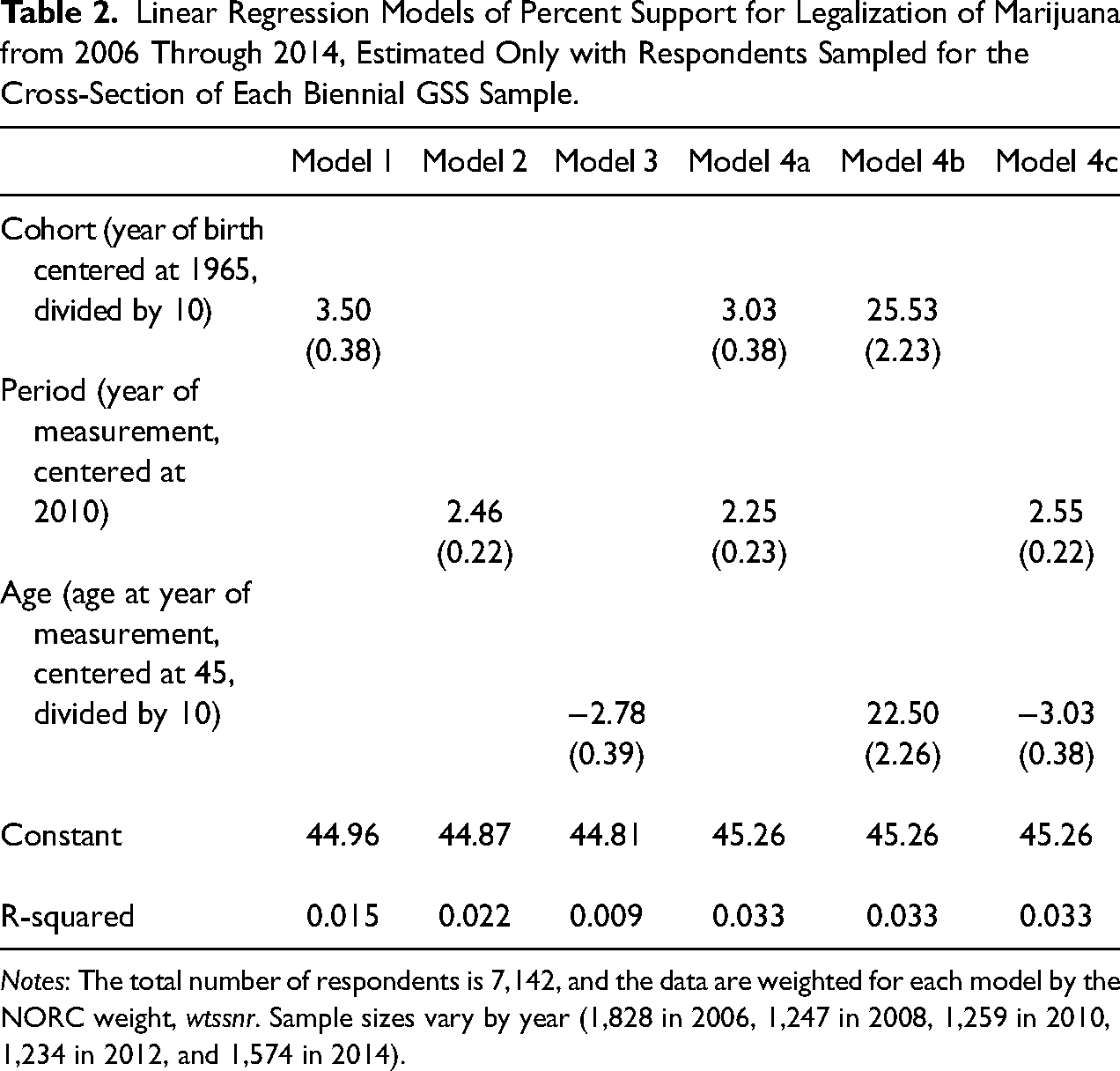
Notes: The total number of respondents is 7,142, and the data are weighted for each model by the NORC weight, wtssnr. Sample sizes vary by year (1,828 in 2006, 1,247 in 2008, 1,259 in 2010, 1,234 in 2012, and 1,574 in 2014).

The estimated coefficients from these models – ${\hat{\beta }}_c$ , ${\hat{\beta }}_p$ , and ${\hat{\beta }}_a$ – can be interpreted as unadjusted naive estimates of cohort, period, and age effects. With the scaling detailed in the row labels of Table 2, the coefficients capture three associations during the observation interval from 2006 to 2014. First, for each decade of difference in birth year, support for legalization was higher by 3.50%. For example, in comparison to those born in 1945, an additional 14% of those born in 1985 supported legalization (i.e., 3.50 * [1985−1945]/10 = 14). Second, for each year from 2006 to 2014, an additional 2.46% of respondents supported legalization, for a total increase of 19.68% over eight years (i.e., 2.46 * [2014−2006] = 19.68). Third, for each decade of difference in age, support for legalization was lower by 2.78%. Thus, in comparison to 30-year-olds, 11.12% fewer 70-year-olds supported legalization (i.e., −2.78 * [70−30]/10 = −11.12).

Most analysts of social change, after estimating three such zero-order associations, would hope to move toward more elaborate models that reveal how much raw change might be attributable to cohort replacement. The most common choice would be to estimate

$$y_i=\hat{\alpha }+{\hat{\beta }}_{c}birth\mathrm{\_}yea{r}_i+{\hat{\beta }}_{p}year\mathrm{\_}of\mathrm{\_}measuremen{t}_i+{\epsilon }_i$$

(4a)

Age is excluded from this model because of the linear dependence of cohort, period, and age, which prevents estimation of a model with all three predictors specified simultaneously. Scholars who have studied the APC literature in more depth know that two alternative specifications of the same model are available:

$$y_i=\hat{\alpha }+{\hat{\beta }}_{c}birth\mathrm{\_}yea{r}_i+{\hat{\beta }}_{a}ag{e}_i+{\epsilon }_i$$

(4b)

and

$$y_i=\hat{\alpha }+{\hat{\beta }}_{p}year\mathrm{\_}of\mathrm{\_}measuremen{t}_i+{\hat{\beta }}_{a}ag{e}_i+{\epsilon }_i$$

(4c)

All three versions of the model are presented in the final three columns of Table 2.

While the regressor specifications differ for the three variants of model 4, the APC literature shows that they are, in fact, the same model from a prediction perspective. In other words, all three specifications generate the same predicted values. As a result, as shown in Table 2, the percentage of variance explained is the same, and the common centering of the three predictors yields the same intercept of 45.26. One could differentiate the models superficially by introducing alternative nonlinear codings for each of the three regressors, but the linear variants of the specifications in models 4a-c reveal the core identification challenge.

How should we interpret the coefficient estimates ${\hat{\beta }}_c$ , ${\hat{\beta }}_p$ , and ${\hat{\beta }}_a$ for model 4, each of which is estimated twice across all three specifications? A natural (if somewhat misleading) interpretation is available for the coefficients from specifications 4a and 4c: support for legalization was increasing in time (measured across periods) while younger respondents (measured by age) who were also from more recent birth cohorts (measured by year of birth) were more likely to support legalization.

The coefficient estimates from specification 4b, in contrast, are not easy to interpret. The key feature of the data – and the reason we have chosen this outcome for detailed explication – is that period-patterned variation in support for legalization is very prominent. Yet, the specification for model 4b does not use period-based design information directly. Thus, for specification 4b, the period-patterned variation is projected simultaneously onto the cohort and age regressors, which have distributions that are evolving across periods. Cohort and age can, in fact, work together to represent period-patterned variation, but the price for doing so is hard-to-interpret coefficient estimates that (misleadingly) imply that more recent birth cohorts and those who are older are both much more likely to support legalization. The target population is progressively composed of more recent birth cohorts, and those birth cohorts are living longer. Model 4b uses these compositional shifts, which are slow moving, to represent the period-patterned variation. In addition, the age coefficient reverses sign, relative to model 4c, because it is estimated alongside year of birth. Any lingering lifecourse-related variation is overwhelmed by the period-patterned variation, which unfolds in the same calendar time as aging. Finally, the joint distribution of age and birth year is constrained (e.g., those born in 1971 must be between the ages of 35 and 43 across the observation interval), and this keeps the predicted values within the 0 to 100 range even though the coefficients are comparatively large.

Altogether, the models in Table 2 are puzzling. A basic pattern in the data is clear from models 1-3. If one were to report model 4a or 4c, then one could claim additional insight. But, if one is forced to reckon with the fact that model 4b is in fact the same model, such claims are less convincing. An analyst cannot claim to have determined how support for legalization has changed because of events during the observation interval, how any such period-based change is patterned alongside the effects of aging, and whether cohort replacement is a complementary source of change.

A Hidden Limitation of the Cross-Sectional Data: The Open-Cohort Structure

Our data setup for the repeated cross-sectional APC results in Table 2 is entirely conventional. We pooled fived realized samples from a survey with a fixed definition of the target population. Nonetheless, this setup presents a hidden challenge that is rarely discussed explicitly in the APC literature, even though the challenge of open cohorts is well known.

For the observation interval of our analysis from 2006 to 2014, the target population of the GSS remained the same: English- and Spanish-speaking adults, aged 18 or older, living at residential addresses in the US. ⁶ The fixed definition of the target population is an explicit constraint on the data, and the constraint is not fully aligned with the research questions typically pursued in an APC analysis.

Consider the 2006 and 2008 GSS surveys as an example of the complexity. The 2008 target population has the same definition as the 2006 target population, but the actual target population shifts because of entry and exit. New entrants include those who aged into the 2008 target population, those who moved from group quarters to residential addresses, those who learned enough English or Spanish to be willing to sit for a GSS interview, and those who were resident outside of the US in 2006 but who moved into residential addresses in the US by 2008. In addition, the 2008 target population excludes members of the 2006 target population who died, entered group quarters, or left the country.

More generally, while adjacent pairs of biennial target populations overlap to a large extent, each birth cohort in each target population is open to multiple types of entry and exit, some of which do not align with the framing of a typical APC analysis. It is not possible to effectively close the cohort structure for repeated cross-sectional studies without detailed retrospective lifecourse data and some hard choices about which types of entry and exit should be given scope to generate cohort-replacement effects. For nearly all APC analyses of the GSS we have read, it would seem that scholars regard entry and exit from cohorts to be defined only by aging into the target population and then dying off from it. The panel data model that we offer in the next section cannot fully solve the “open cohort” challenge, but some of the dynamics that arise from entry and exit can be controlled more completely.

A Rolling Panel Data Model of Cohort, Period, and Aging Effects

In this section, we offer our proposed model, analyzing GSS respondents sampled in 2006, 2008, and 2010 who were re-interviewed two and four years later (from 2008 through 2014; see Figure 1 above). Although we will defer a full discussion of the identification assumptions of the model until after we present results and the types of substantive conclusions that they can suggest, three key features of the design of the GSS treble panel make our modeling approach possible. First, the GSS samples from the full adult age structure living in households, thereby supplying full variation in age and year of birth at the time of sampling during the observation interval. Second, the GSS panels directly measure the outcomes of interest at three different ages for each respondent. Third, the three GSS panel samples overlap within the observation interval, and this overlap allows for the separation of aging effects from period effects during the observation interval, conditional on maintained assumptions and the fitting of cohort effects that carry forward the effects of age and period differences from before the observation interval.

The treble panel, nonetheless, presents some additional practical challenges for modeling. Beyond the cohort closure decisions discussed above, with this data configuration we must also contend with non-random panel attrition (see Morgan and Lee 2020). We discuss in the appendix how we used weighting procedures to adjust for panel attrition while imposing an appropriate level of closure on the cohorts for our analysis.

The Alternative Panel Data Model, Compared to a Traditional Underidentified APC Model

To link our results directly to the traditional APC estimates from Table 2, we first offer two analogs to the cross-sectional models 1 and 2 as models 1p and 2p in Table 3:

$$y_{it}=\hat{\alpha }+{\hat{\beta }}_{c}birth\mathrm{\_}yea{r}_i+{\epsilon }_{it}$$

(1p)

$$y_{it}=\hat{\alpha }+{\hat{\beta }}_{p}year\mathrm{\_}of\mathrm{\_}measuremen{t}_{it}+{\epsilon }_{it}$$

(2p)

Table 3.

Panel Linear Regression Models of Percent Support for Legalization of Marijuana from 2006 Through 2014, Estimated Only with Respondents Sampled in 2006, 2008, and 2010 Who Were Followed-Up Biennially Through 2010, 2012, and 2014, Respectively.

	Model 1p	Model 2p	Model 5	Model 6	Model 7	Model 8
Cohort (year of birth centered at 1965, divided by 10)	2.83			2.56	2.56
	(0.62)			(0.62)	(0.62)
Cohort groups (reference: before 1946)
Boomers (1946-65)						15.84
						(2.79)
Generation X (1966-81)						14.28
						(2.88)
Millennials (after 1981)						16.03
						(3.48)
Period (year of measurement, centered at 2010)		3.11		4.15
		(0.34)		(0.64)
Periods (reference: 2006)
2008					5.33	5.51
					(2.23)	(2.23)
2010					15.82	16.12
					(2.92)	(2.91)
2012					22.58	22.92
					(4.09)	(4.07)
2014					32.49	32.89
					(5.13)	(5.10)
Aging (centered panel years: -2, 0, or 2)			1.95	-2.26	-2.26
			(0.28)	(0.71)	(0.72)
Aging by cohort group:
Aging for pre-boomers						-3.90
						(0.83)
Aging for boomers						-2.32
						(0.76)
Aging for generation X						-1.87
						(0.88)
Aging for millennials						-1.61
						(1.04)
Constant	45.63	44.93	45.06	45.40	30.31	16.71
R-squared	0.009	0.021	0.004	0.031	0.032	0.038

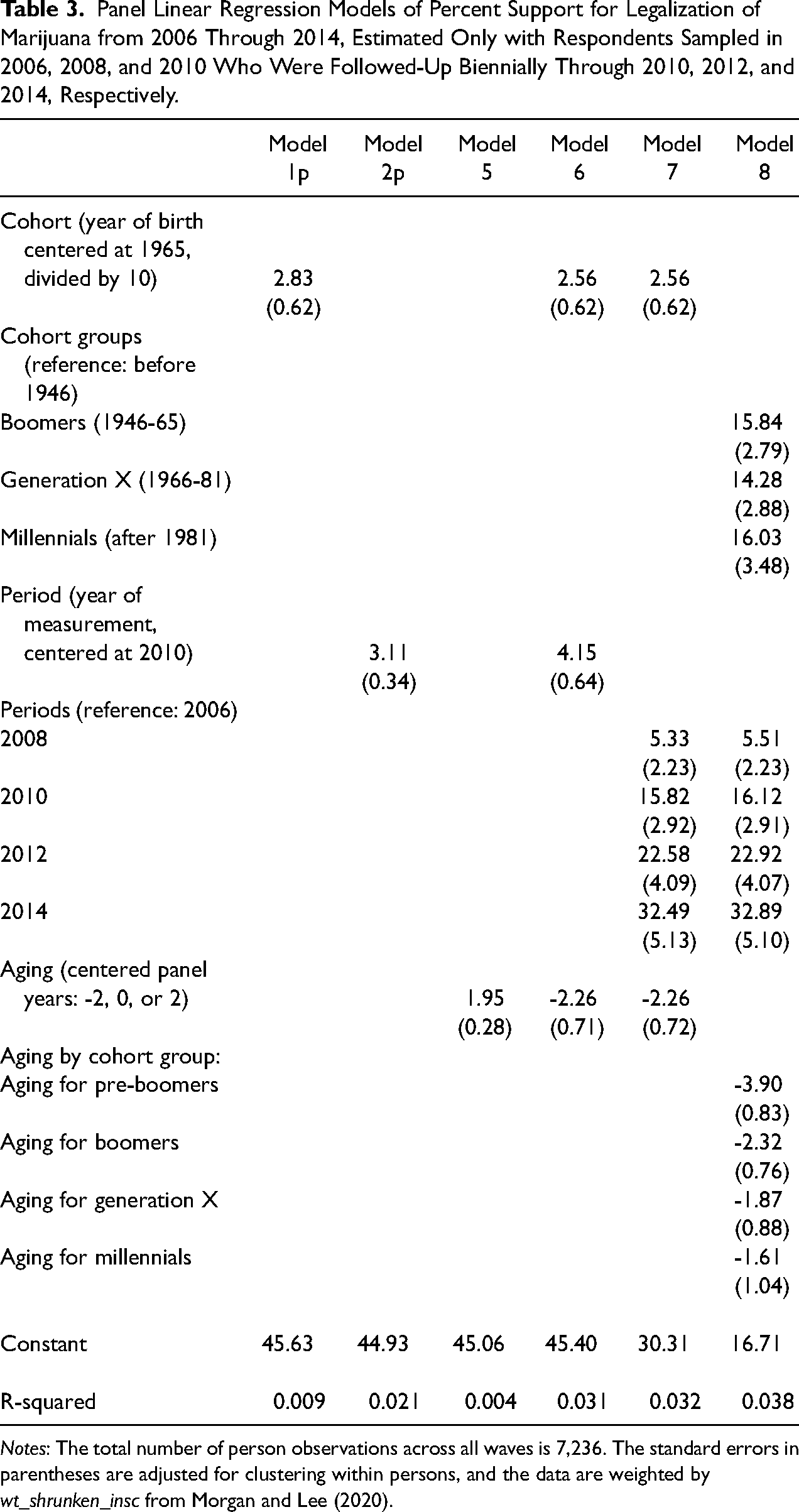
Notes: The total number of person observations across all waves is 7,236. The standard errors in parentheses are adjusted for clustering within persons, and the data are weighted by wt_shrunken_insc from Morgan and Lee (2020).

For these models, ${\hat{\beta }}_c$ and ${\hat{\beta }}_p$ can be given similar interpretations as for models 1 and 2 because (a) the data span the same observation interval from 2006 to 2014 and (b) the models do not incorporate our design knowledge that each respondent contributes three observations. The coefficients are, in fact, similar to those from models 1 and 2, in the sense that both pairs of coefficients suggest that cohort and period change contributed to raw change. Nonetheless, as we discussed just above, the target population is different for this configuration of the GSS data, and this difference likely contributes to a smaller association with cohort.

In Table 3, we do not offer a model 3p that is an analog to model 3 in Table 2. Instead, we use panel wave (specified in years as −2, 0, and 2 for each three-wave, four-year panel) in order to define a new “aging” predictor. We therefore offer instead a new model 5:

$$y_t=\hat{\alpha }+{\hat{\beta }}_{a}agin{g}_{it}+{\epsilon }_{it}$$

(5)

where now ${\hat{\beta }}_a$ is what we will label an unadjusted naive estimate of an aging effect, averaged over individuals in the three panels simultaneously. The estimated coefficient of 1.95 is a particularly poor estimate of an aging effect. It uses an index of aging that is absolutely straightforward – all respondents age by 2 years between each wave of the panel – but it ignores the placement of each individual's aging within the periods defined by calendar time (e.g., from 2006 to 2010, or from 2008 to 2012, or from 2010 to 2014, which is set by the panel design). As a result, the total association summarized by ${\hat{\beta }}_a$ from model 5 is misleading because it does not differentiate between period variation and the portion of within-respondent variation that is attributable to aging within the lifecourse.

Model 6 is our key model, and it specifies simultaneously the three regressors from models 1p, 2p, and 5:

$$y_{it}=\hat{\alpha }+{\hat{\beta }}_{c}birth\mathrm{\_}yea{r}_i+{\hat{\beta }}_{p}year\mathrm{\_}of\mathrm{\_}measuremen{t}_{it}+{\hat{\beta }}_{a}agin{g}_{it}+{\epsilon }_{it}$$

(6)

The estimated coefficients for ${\hat{\beta }}_c$ , ${\hat{\beta }}_p$ , and ${\hat{\beta }}_a$ suggest three related findings. First, for each decade of difference in birth year, support for legalization was higher by 2.56%. Second, for each year from 2006 to 2014, an additional 4.15% of respondents supported legalization. Third, for each year of aging, during the observation interval, support for legalization was lower by 2.26%. Considered together, the aging effect during the observation interval is countervailing, and thus, the period effect is larger than was suggested by model 2p.

We will provide below a full discussion of how to understand this model, embedded within a comparison to the more traditional APC analysis presented above in Table 2. However, we should first explain why model 6 can be estimated from the observed data. Unlike a three-regressor APC model with repeated cross-sectional data, the rolling panel data model is identified in a narrow technical sense because the design matrix set by the right-hand-side of Equation (6) is full rank. In particular, our index of aging variation is independent of cohort because all respondents participate in the panel for three waves, regardless of the year in which they were born. Period variation and between-wave aging variation are not independent because later waves are also later years in calendar time. But, we have overlapping panels, and thus, the design generates separable variation in both period and aging.

Consider Figure 2, which depicts the ages and aging of a single cohort of GSS respondents, born in 1971, as they passed through the GSS treble panel design. The cohort members are observed in three configurations, as they age from 35 to 39 for the first panel, from 37 to 41 for the second panel, and from 39 to 43 for the third panel. The overlap of the panels across the periods of the observation interval ensures that our aging regressor has variance that cannot be reduced to the measured values of age. As more fully explained below, we capture the separable identifying information in Figure 2 by the particular aging regression specification we adopt above. To justify using such a specification, we must assume that the effect of aging does not vary across the three four-year subintervals of the full observation interval.

Figure 2.

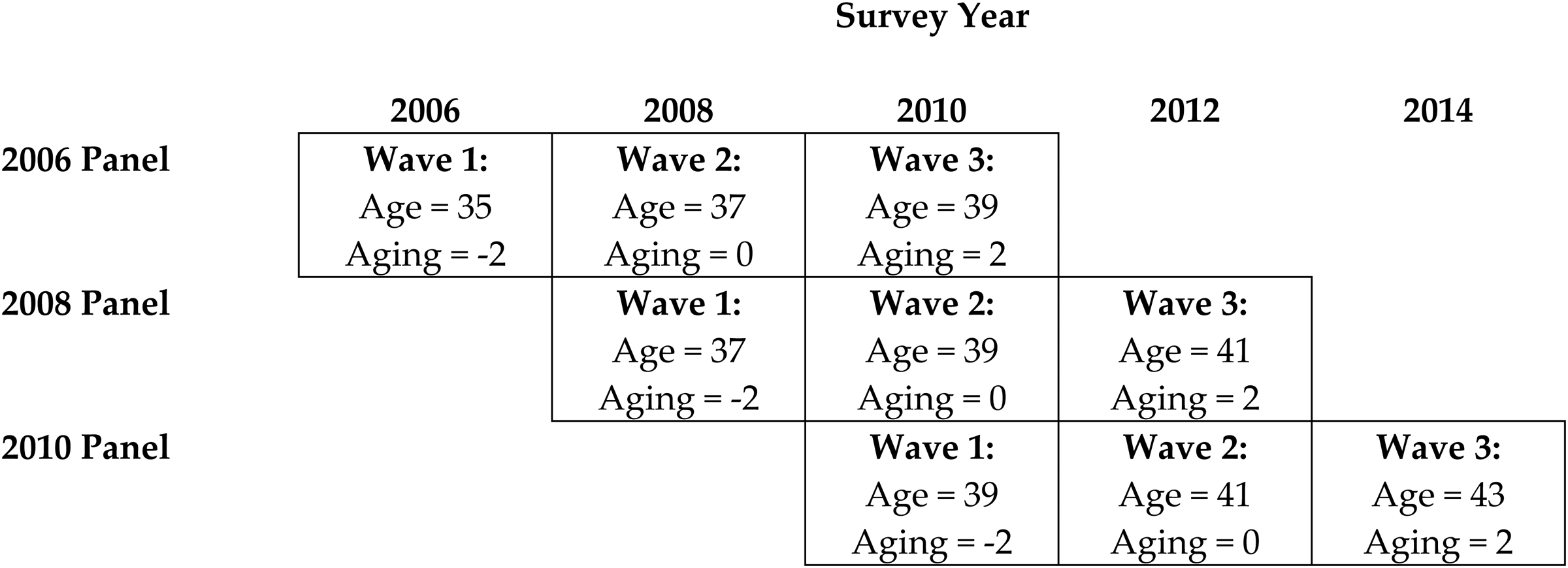
Age and aging variation for the 1971 birth cohort.

Additional Specifications with Additional Outcomes for Comparison

Our full explanation below will be clearer after we offer a wider range of estimated models and the types of interpretations that they suggest. Accordingly, in this subsection, we elaborate the parameterization of cohort, period, and aging effects for the legalization of marijuana with nonlinear and interactive coding. We then offer estimated models for six additional outcomes.

For model 7 in Table 3, period is given a fully nonlinear coding: indicator variables for each biennial year of observation, with the first-year, 2006, as the omitted reference. While model 6 suggests a linear increase of 33.2% (4.15 percent for each of 8 years), model 7 shows that the increase was smallest for the first interval from 2006 to 2008.

Model 8 introduces a nonlinear coding of cohort, while relaxing the implicit constraint that variation in the aging effect is unrelated to cohort. First, we collapse years of birth to four common “generation” definitions. We therefore set up comparisons of boomers (born 1946-1965), Generation X (born 1966-1981), and Millennials (born after 1981) to a more heterogenous reference generation born before 1946, which we label “pre-boomers.” We also enter the aging variation into the model with a simple but complete generation-based decomposition using four separate regressors. After coding aging variation with the same −2, 0, and 2 values used above, we cloned the variable for each generation. We then set the value of each regressor to 0 if the respondent was not in the corresponding generation. These four regressors thus represent the full set of aging variation in four pieces – one for each generation – and model 8 substitutes all four aging regressors for the single aging regressor of models 6 and 7.

Like model 7, model 8 shows that period-estimated change does not depart greatly from linearity. However, model 8 shows a substantial non-linearity for cohort, suggesting a pronounced generation-based difference between those born before 1946 and those born after. In addition, the aging effect varies by cohort, which suggests that the aging-based decline in support for legalization, net of the overall period effects estimated at the same time, is strongest for the oldest generation. The aging effect weakens progressively for the more recent generations, who were observed during earlier ages while in the observation interval.

Our overall interpretation of model 8 is that period variation in support for legalization is the dominant source of change between 2006 and 2014. This change was complemented by shifts in the composition of cohorts. At the same time, the period-based source of change was held back to some extent by the slight propensity for individuals to reduce their support for legalization as they aged. This countervailing aging effect was strongest for older generations, who are apparently the least comfortable with change, especially during an observation interval when change was widely supported by younger individuals.

At this point, we expect some readers to wonder whether the countervailing aging effect is sensible or whether it is some artifactual consequence of the simultaneous estimation of cohort, period, and aging effects. The intuition of such a suspicion is correct, but it should be embraced not eschewed. The point of the APC literature is to allow for aging effects that are generated by between-age differences during an observation interval, and which are estimated simultaneously alongside differences attributable to both between-period change and cohort differences that evolve because of population replacement. In other words, the point of using regression modeling is precisely to (a) separate these effects and (b) use them in combination to offer joint interpretations of raw change. If one is uncomfortable with the resulting estimates (or suitable combinations of them), then the discomfort arises not from the APC problem, nor the rolling panel data, but rather the choice to embrace the goal of decomposing sources of raw change with regression methodology. (We will return to discuss this point below.)

Tables 4 to 6 present estimates of models 6-8 for the remaining six outcomes. For Table 4, the three models are estimated for two measures of approval for same-sex relations. Change in these outcomes is structured, in the main, just as for support for the legalization of marijuana, although with some subtle differences of note. First, cohort-based change, when coded by generation, is relatively smooth for these outcomes during the observation interval. The countervailing aging effect is also weaker, with less evidence of variability by cohort, and with the threshold for such variability at the Millennial generation. Finally, for approval of same-sex marriage, the period-based change is particularly pronounced between 2010 and 2014, which is the interval when legislative changes and legal developments were most prominent, especially at the state level.

Table 4.

Panel Linear Regression Models of Percent Support for Same-Sex Relations from 2006 Through 2014, Estimated Only with Respondents Sampled in 2006, 2008, and 2010 Who Were Followed-Up Biennially Through 2010, 2012, and 2014, Respectively.

	Support for the Position That Same-Sex Sexual Relations Are Not Wrong at All			Support for Same-Sex Marriage
	Model 6	Model 7	Model 8	Model 6	Model 7	Model 8
Cohort (year of birth centered at 1965, divided by 10)	5.35	5.35		5.38	5.37
	(0.61)	(0.61)		(0.59)	(0.59)
Cohort groups (reference: before 1946)
Boomers (1946-65)			10.77			9.25
			(2.65)			(2.56)
Generation X (1966-81)			20.73			17.80
			(2.82)			(2.75)
Millennials (after 1981)			26.28			29.27
			(3.73)			(3.54)
Period (year of measurement, centered at 2010)	2.66			3.91
	(0.63)			(0.60)
Periods (reference: 2006)
2008		7.03	7.27		3.10	3.18
		(2.21)	(2.23)		(2.25)	(2.25)
2010		11.44	11.70		10.07	10.26
		(2.85)	(2.86)		(2.84)	(2.84)
2012		16.78	17.08		20.16	20.28
		(4.02)	(4.03)		(3.92)	(3.91)
2014		22.18	22.51		29.95	30.15
		(5.17)	(5.18)		(4.89)	(4.88)
Aging (centered panel years: -2, 0, or 2)	-1.69	-1.69		-1.75	-1.73
	(0.68)	(0.68)		(0.69)	(0.68)
Aging by cohort group:
Aging for pre-boomers			-1.71			-2.02
			(0.77)			(0.86)
Aging for boomers			-1.69			-2.09
			(0.75)			(0.75)
Aging for generation X			-2.43			-2.10
			(0.83)			(0.91)
Aging for millennials			-0.47			0.03
			(0.98)			(0.95)
Constant	42.16	30.59	14.37	46.28	34.43	19.30
R-squared	0.042	0.042	0.042	0.055	0.057	0.059

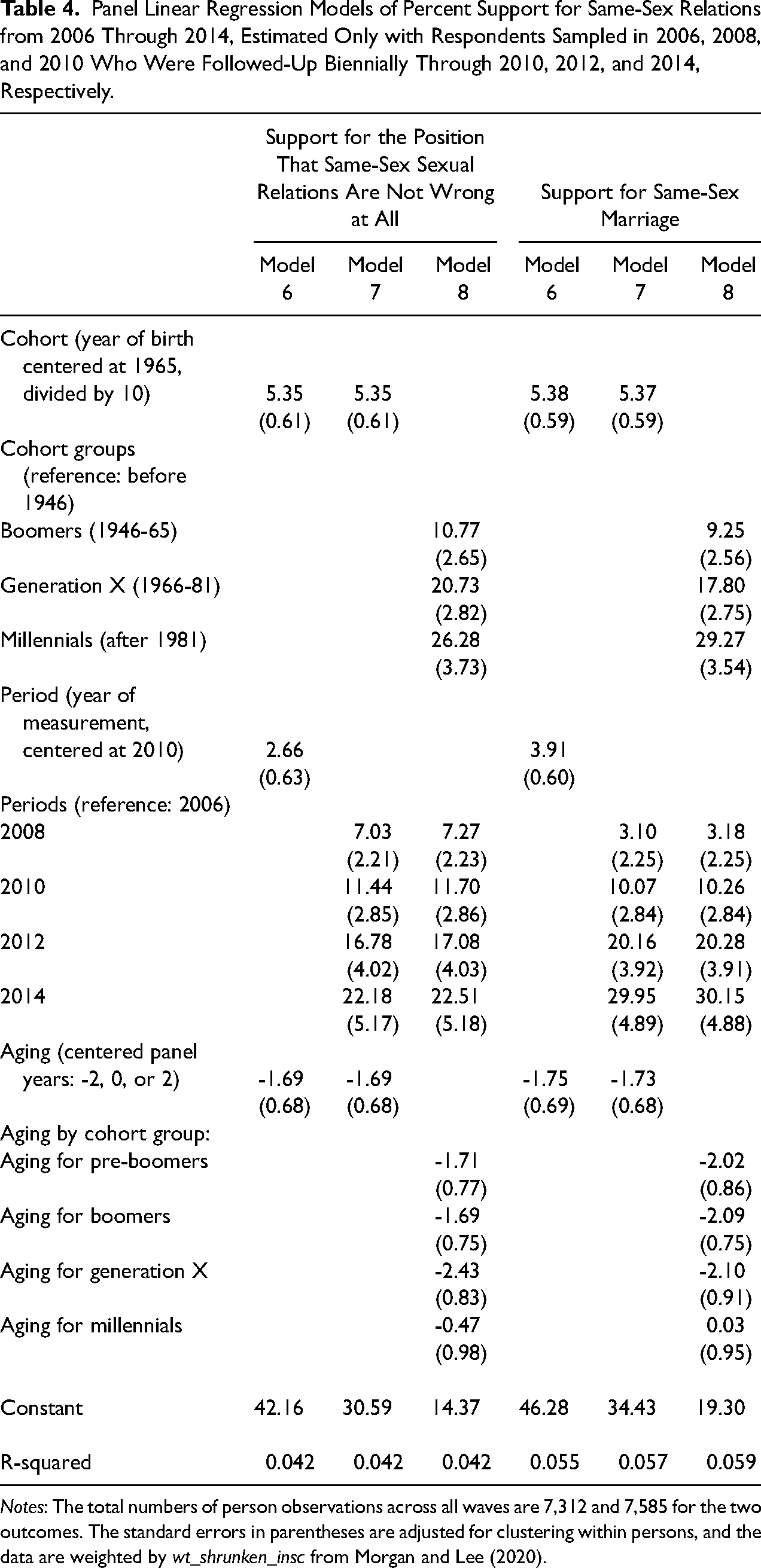
Notes: The total numbers of person observations across all waves are 7,312 and 7,585 for the two outcomes. The standard errors in parentheses are adjusted for clustering within persons, and the data are weighted by wt_shrunken_insc from Morgan and Lee (2020).

Overall, approval of same-sex sexual relations and marriage shows strong period and cohort-based change during the observation interval, with a smaller countervailing effect of within-person aging. For cohort replacement, the generational coding suggests a smooth succession of more supportive cohorts. This pattern departs from the cohort-replacement pattern for support for the legalization of marijuana, where cohort change was probably carrying forward only a lagged period-and-coming-of-age effect, the “Age of Aquarius” or “the-sixties-changed-everything” (see Davis 2004).

Table 5, in contrast, shows patterns for outcomes that have distinct nonlinear period changes. Self-rated improvement in one’s financial situation declined rapidly from 2006 to 2010, before rising slightly in 2012 and 2014. This pattern reflects the timing of the Great Recession, as well as the relatively slow recovery that followed. This non-linear period-based change is revealed by the model even though the lifecourse dynamics picked up by cohort and aging continued as expected. More recent cohorts, who were younger at the time of entry into the observation interval, were more likely to experience improvement in their financial situation. They were the cohorts whose careers were unfolding with accruing seniority. Furthermore, aging had a sizable positive relationship for the youngest generation, whose financial situations were improving most swiftly as they entered into the labor force and established financial independence in their 20s and early 30s. The model reveals these lifecourse patterns alongside the co-occurring and disruptive period-patterned change that was produced by the Great Recession.

Table 5.

Panel Linear Regression Models Equivalent in Structure to Those in Table 4, but for Two Outcomes with More Variable Aging Effects and Sudden Period Effects.

	Financial Situation Has Been Getting Better			Need More Spending on Health
	Model 6	Model 7	Model 8	Model 6	Model 7	Model 8
Cohort (year of birth centered at 1965, divided by 10)	6.18	6.17		1.39	1.39
	(0.36)	(0.36)		(0.42)	(0.42)
Cohort groups (reference: before 1946)
Boomers (1946-65)			9.46			9.04
			(1.50)			(2.00)
Generation X (1966-81)			23.10			7.61
			(1.77)			(2.14)
Millennials (after 1981)			27.62			8.79
			(2.13)			(2.40)
Period (year of measurement, centered at 2010)	−1.40			−1.65
	(0.37)			(0.44)
Periods (reference: 2006)
2008		−9.86	−9.50		5.40	5.53
		(1.96)	(1.98)		(1.77)	(1.77)
2010		−17.72	−17.09		−9.70	−9.44
		(2.12)	(2.15)		(2.20)	(2.19)
2012		−14.35	−13.63		−4.99	−4.78
		(2.55)	(2.59)		(2.86)	(2.85)
2014		−12.34	−11.58		−9.33	−9.20
		(3.14)	(3.19)		(3.67)	(3.66)
Aging (centered panel years: -2, 0, or 2)	0.79	0.77		−0.98	−0.99
	(0.46)	(0.46)		(0.52)	(0.52)
Aging by cohort group:
Aging for pre-boomers			0.42			−2.14
			(0.63)			(0.74)
Aging for boomers			0.28			−1.14
			(0.57)			(0.59)
Aging for generation X			0.04			−0.96
			(0.65)			(0.67)
Aging for millennials			2.94			0.29
			(0.98)			(0.97)
Constant	32.28	44.93	27.81	65.76	69.92	62.33
R-squared	0.051	0.059	0.056	0.013	0.023	0.025

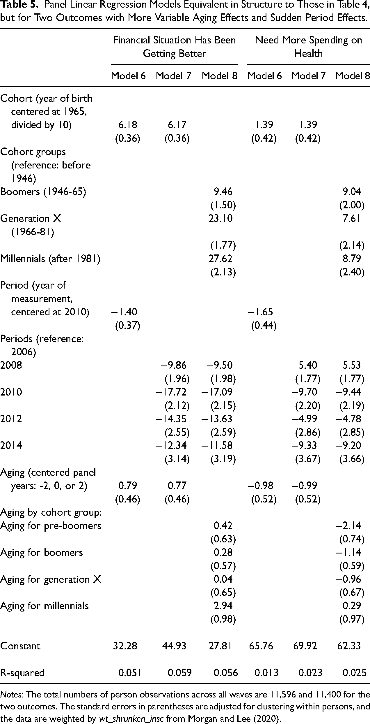
Notes: The total numbers of person observations across all waves are 11,596 and 11,400 for the two outcomes. The standard errors in parentheses are adjusted for clustering within persons, and the data are weighted by wt_shrunken_insc from Morgan and Lee (2020).

Table 5 also shows that support for additional national spending on health hit a low point in 2010. From a 2008 high, when both Clinton and Obama ran on the need for healthcare reform, support for increased health spending fell by 15% following the passage of the Affordable Care Act in spring 2010 (see also Morgan and Kang 2015). After 2010, support moved up and down as the value of Obamacare continued to be debated. Cohort differences resemble those for the legalization of marijuana, with the pre-baby-boom generation as the outlier, feeling least interested in the need for more health spending. This cohort effect was reinforced by negative aging effects among cohorts with older respondents during the observation interval, which is consistent with age-based differences in satisfaction with employer-based health plans among middle-aged respondents and fears among older respondents that resources for Medicare could become compromised.

Table 6 offers two final comparisons that show how the model performs when period-based change is small. Raw support for spending on education has increased over the years, and Table 6 suggests that this change is driven primarily by cohort differences and their evolution in time, matching results from the existing literature (e.g., Plutzer and Berkman 2005). As more recent cohorts have accumulated more education, they have supported more spending on education in general. For aging-related change, Millennials, who were more likely to still be accumulating education during the observation interval, were the only respondents to display an aging effect. Net of their overall cohort effect, they supported increases in education spending, perhaps on their own educational opportunities during an era of higher college tuition and a growing awareness of the totality of their own expenses. Middle-age and older respondents, from earlier generations, showed no such propensity during the observation interval. Finally, net of cohort-driven change, and the possibly-self-serving aging effect of younger adults, the model offers no evidence of period-based change.

Table 6.

Panel Linear Regression Models Equivalent in Structure to Those in Table 4, but for Two Outcomes with That Have Much More Modest Change, Associated Primarily with Cohort Replacement and Variable Aging Effects.

	Need More Spending on Education			Vocabulary Knowledge
	Model 6	Model 7	Model 8	Model 6	Model 7	Model 8
Cohort (year of birth centered at 1965, divided by 10)	2.50	2.50		−0.11	−0.11
	(0.40)	(0.40)		(0.03)	(0.03)
Cohort groups (reference: before 1946)
Boomers (1946-65)			6.24			-0.00
			(1.89)			(0.12)
Generation X (1966-81)			10.92			-0.31
			(1.98)			(0.13)
Millennials (after 1981)			11.06			-0.51
			(2.23)			(0.14)
Period (year of measurement, centered at 2010)	0.10			-0.00
	(0.41)			(0.02)
Periods (reference: 2006)
2008		1.67	1.87		-0.16	-0.17
		(1.88)	(1.87)		(0.10)	(0.10)
2010		2.11	2.49		-0.15	-0.15
		(2.12)	(2.11)		(0.12)	(0.12)
2012		2.01	2.42		-0.14	-0.14
		(2.75)	(2.74)		(0.16)	(0.16)
2014		0.87	1.26		-0.13	-0.13
		(3.39)	(3.38)		(0.20)	(0.20)
Aging (centered panel years: -2, 0, or 2)	-0.01	-0.01		0.05	0.05
	(0.48)	(0.48)		(0.03)	(0.03)
Aging by cohort group:
Aging for pre-boomers			-0.22			-0.02
			(0.75)			(0.04)
Aging for boomers			-0.89			0.05
			(0.56)			(0.03)
Aging for generation X			0.06			0.06
			(0.58)			(0.03)
Aging for millennials			1.64			0.08
			(0.87)			(0.04)
Constant	75.15	73.53	65.18	6.08	6.22	6.43
R-squared	0.009	0.009	0.009	0.010	0.010	0.012

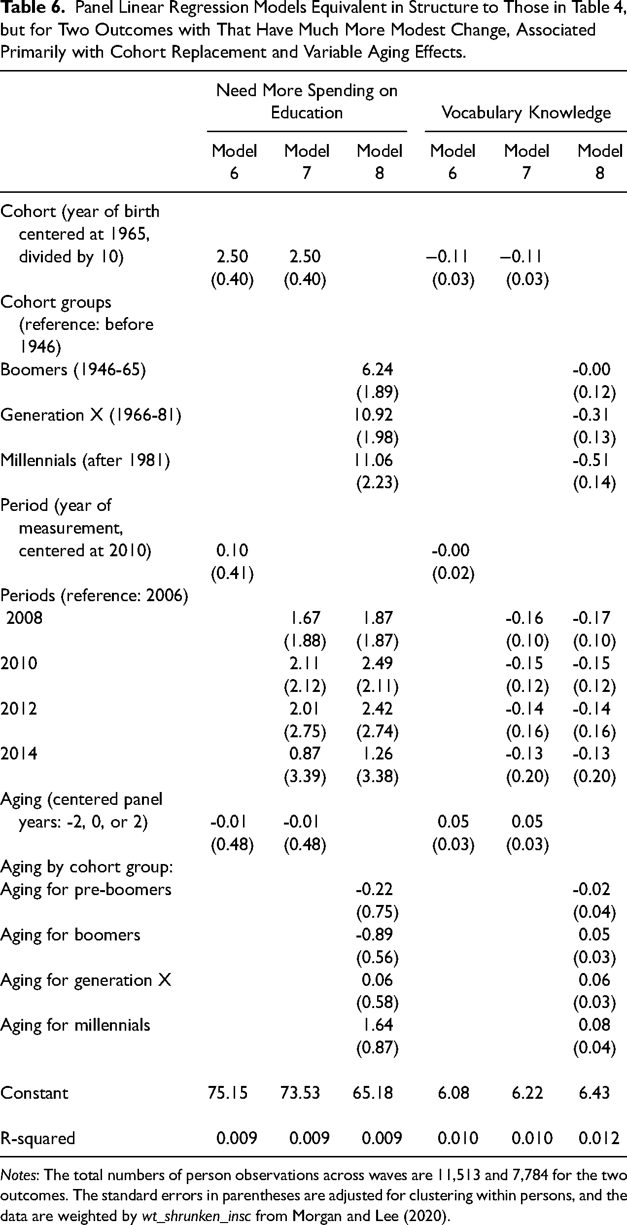
Notes: The total numbers of person observations across waves are 11,513 and 7,784 for the two outcomes. The standard errors in parentheses are adjusted for clustering within persons, and the data are weighted by wt_shrunken_insc from Morgan and Lee (2020).

We offer also in Table 6 models for the GSS vocabulary test that has been analyzed extensively in the APC literature. Note first that the scaling of this outcome is much different: a correct score on a 0-to-10 scale, rather than differences in percent that vary from 0 to 100. As such, the coefficients are smaller in magnitude. Substantively, the model shows no evidence of period-based change (with perhaps a small anomalous difference for 2006). The model does, however, provide evidence of cohort-based change. In particular, boomers and those born earlier scored better on the vocabulary test than more recent cohorts, net of very small age-related differences which suggest that younger respondents gain small amounts of vocabulary knowledge, perhaps as some of them continued to accumulate education. The cohort difference, however, is not what one might have expected – unless one knows the pre-existing literature on this outcome. The more recent cohorts have smaller vocabularies, which is thought by some researchers to be attributable to prior period differences embedded earlier in the lifecourse, such as the declining complexity of reading texts used in elementary and middle schools (Hayes, Wolfer, and Wolfer 1996), perhaps complemented by other changes in attitudes toward reading (Glenn 1994).

Altogether, Tables 3 through 6 demonstrate that the panel data models can suggest a variety of patterns of change. For support for the legalization of marijuana and same-sex relations, period effects are strong, and cohort replacement plays an important complementary role. Aging effects are countervailing to varying degrees, net of overall average period-based change. For nonlinear, period-based change, such as self-rated financial situation and support for additional health spending, the models can reveal the nonlinearities when parameterized effectively. For these examples, no single source of change – whether cohort, period, or aging – is dominant. Finally, when period-related change is small or non-existent, such as for support for additional education spending or for vocabulary knowledge, cohort replacement can still drive raw change, either relatively large change, such as for education spending, or small but meaningfully counterintuitive change such as for vocabulary knowledge.

In the next section, we justify the interpretations we have offered of the panel data models, detailing the core assumptions on which they rest. Before doing so, we wish to point the reader to a few additional models that are provided in the appendix. Table A1 offers models that demonstrate how two alternative but reasonable choices for modeling are inconsequential for our results – using logit models rather than least-squares models and handling missing values on the outcomes differently. Table A2 offers fixed-effect, panel data models to show why they are of limited utility in this context, even though they may be useful for evaluating the position that all raw change can be attributed to cohort replacement.

Identification and Interpretation of the Rolling Panel Data Model

For the results generated by the rolling panel data model above, we interpreted the estimated period effects as net population-averaged change in the outcome during the observation interval, adjusted for underlying aging effects that could either be reinforcing or countervailing. In addition, we interpreted the estimated cohort effects as differences that contribute to raw change because of how the composition of cohorts evolves during the observation interval. And, as first indicated in the introduction, we regard the estimated cohort effects, most fundamentally, as the joint effects during the observation interval of entangled period and cumulated aging differences from before the observation interval.

In this section, we aim to justify interpretations of this type. Doing so requires that we offer a careful comparison with the rationale for undertaking a traditional APC analysis with repeated cross-sectional data using the accounting-model setup of Mason et al. (1973) and Fienberg and Mason (1979). After detailing the estimands, we then present the identification assumptions that justify our model interpretations.

Characterization of the Estimands of Interest

For the APC literature that has considered how to analyze repeated cross-sectional data (or pooled data variants), the traditional accounting-model setup defines effect parameters for age, period, and cohort as additive constants that generate an outcome. The specified effects are assumed to be inherently confounded because of the linear dependence of the age, period, and cohort variation. In practice, empirical models are usually specified with indicator-variable regressors for segments of the observed range of each variable for age, period, and cohort. Cross-product interactions are excluded because of the particular additivity constraint of the accounting model.

To explore some implications of the accounting-model setup, consider age and period effects in early adulthood. ⁷ These effects can only be estimated with data on the joint support of observed age and period variation. The support of the age data is usually straightforward. For the GSS, for example, each sample includes respondents from ages 18 to “89 or older.” The support of the period data is constrained by the observation interval. Suppose for this discussion of the accounting-model setup in this section that we were analyzing the full GSS cumulative file from 1972 to 2018. With this choice, elderly respondents who were sampled during the first time periods observed would have experienced their early adulthood aging many decades before any of the analyzed GSS data were collected.

Should the analyst regard early adulthood age effects that have been estimated on the support of the period data as relevant to cohorts whose actual early adulthood aging occurred before the observation interval, perhaps decades earlier? This may seem to be an interesting, but secondary, question, given that the primary goal of APC modeling is to understand only the patterns for an outcome during an observation interval selected. In fact, this early-adulthood question is a conundrum when (1) it is recognized how differently prior period and aging differences are sometimes treated by APC analysts who adopt an accounting-model setup and (2) in view of a long-recognized position in the literature that cohort effects can be seen, at their core, as effects that are attributable to interactions between period and age effects (see Ryder 1965; Keyes et al. 2010).

By our reading of the literature, APC analysts who embrace the accounting model are very much interested in developing conclusions about how period differences from before the observation interval determine the outcome of interest during the observation interval. Even Mason et al. (1973), when proposing the accounting model, presented an example of early adulthood cohort effects on party identification:

This suggests that the political environment in which a particular birth cohort first enters the electorate may help determine the extent to which individuals in that cohort identify with a political party for the remainder of their lives. As that party experiences normal fluctuations in political fortunes, however, some members of the cohort may temporarily shift their loyalties. Both cohort and short-term period effects can thus contribute to party identification. Since the aging process might also independently affect party identification (as persons become more “conservative” with age, for example, they may find the Republicans increasingly attractive), we have here another example in which age, period, and cohort conceptually have distinct causal impacts on the dependent variable (Mason et al. 1973:244-46).

These early adulthood sources of cohort effects must have occurred in periods that preceded the observation interval for at least some of the individuals in the data sources that Mason and colleagues were proposing be analyzed with their framework.

Following such thinking, it seems most common in the APC literature to assume that prior period differences are embedded in the cohort differences that have effects during the observation interval. And, under this conceptualization, the cohort effects that are estimated on the support of the data must be interpreted as carrying forward generative period differences that are off the support of the period data.

Now, return to early adulthood age effects more generally and the complications they present. One possible rationalization of the estimands for the accounting-model setup would be to assert that its age and cohort estimands apply with full generality to all members of all of the cross-sectional samples in all periods, including for periods before the observation interval. Taking this approach would require assuming that it is reasonable to extrapolate backward all age and cohort estimands to periods off the support. While there may be law-like biological processes that could justify extrapolation of age estimands for health-related outcomes, it is hard for us to conceive of a rationale for extrapolating cohort estimands in this way for any type of outcome. Cohort differentiation is generated by events in particular periods, and resulting effects can have pronounced latency. Moreover, this rationalization would contradict the emergent position, detailed in Keyes et al. (2010) and Luo and Hodges (2020b), that age effects should be understood as always varying by period, at least potentially, or else the cohort differentiation that generates cohort effects cannot itself emerge.

A related rationalization would be to start with a position similar to ours for the rolling panel data model above: allow the cohort differences during the observation interval to carry forward past entangled period and cumulated aging differences from before the observation interval. The analyst would then assume for the observation interval that the cohort effects have been adjusted effectively by simultaneous estimation of age effects during the observation interval.

Even if full identification were achievable, we believe that this second rationalization is incoherent for the following reasons. If cohort differentiation of consequence were itself generated by interacting period and age effects prior to the observation interval, then a structure of additive age and period estimands for a later observation interval would be very unlikely to encode the prior interactive period and age effects. Thus, it would be, for us, unreasonable to assume that an estimated age effect fit on the support of the data could then “net out” an appropriate amount of each cumulated aging effect, yielding an estimate of a pure structural cohort effect that only carries forward the effect of a past structural period effect. Instead, the estimated age effects would best be considered age-outcome associations for the observation interval, net of cohort effects that carry forward prior cumulated age effects that are yoked to prior period effects. If so, the genuine total age effects would then be split in unknown proportions across both the estimated age effects and the estimated net cohort effects. Such a split is inconsistent with the accounting model itself, which stipulates additive cohort and age effects.

Altogether, we believe that the accounting-model setup, on which a voluminous literature is built, does not provide a satisfactory grounding for its own suggested estimands, once prior period effects are permitted to structure consequential cohort differences that have effects during the observation interval. We are therefore convinced, alongside other appeals in the APC literature (e.g., Luo and Hodges 2020b), of the need for a reconsideration of how to define estimands for cohort effects in the sociological and public opinion literatures.

To conclude this discussion, we return to our interpretations. Our approach can be seen as an extension of past public opinion research in which cohort replacement effects are analyzed with repeated cross-sectional data alongside the analysis of “intracohort change” (see Davis 2001, 2013; Firebaugh 1989, 1997). With rolling panel data, we are better able to model “intracohort change” as simultaneous aging and period effects during the observation interval, alongside cohort effects that we assume carry forward entangled aging and period differences from before the observation interval.

To be absolutely clear on this point, consider the example of individuals who were sampled for the GSS treble panel at age 60 in 2006 (i.e., the oldest members of the baby boom generation that begins with those born in 1946). Under our conceptual setup, we do not attempt to use the differences between those aged 18 and 35 in our data, collected between 2006 to 2014, in order to infer early adulthood aging effects for these 60-year-olds, whose early adulthood aging actually unfolded between 1964 and 1981. Instead, we assume that these prior period differences interacted with prior lifecourse aging differences to generate combined cohort differences. These entangled differences then generate boomer cohort effects during the observation interval, and our models estimate these cohort effects.

From the vantage point of the APC accounting model, we therefore do not attempt to identify structural cohort estimands of the sort that the accounting model defines. Indeed, we take the position that those cohort estimands are ill-defined because the accounting model has too few degrees of freedom to adequately represent the empirical patterns it was developed to elucidate (e.g., the party identification example quoted above from Mason et al. 1973). ⁸ Whether the additional degrees of freedom offered up by the rolling panel data we analyze can be put to good use depends on the assumptions that must be invoked to use them.

Maintained Assumptions That Justify the Identification Claims

We can now return to discuss with precision the key maintained assumptions that allow us to offer the interpretations of the panel data models in the results above. ⁹ We claim that our interpretations of models 6 through 8 above are justified by three assumptions:

• Assumption 1: The aging effects can be estimated as net average associations over short intervals in samples that include individuals of all ages.

• Assumption 2: The aging effects do not vary across subintervals of time within the observation interval.

• Assumption 3: The aging effects are interpretable because it is reasonable to accept that they are conceptually separable from population-averaged period effects.

The first and third assumptions are needed to attach meaning to the coefficient estimates, and the second assumption is the pivotal identification assumption.

For the first assumption, one must accept that overall aging effects on attitudes and opinions can be recovered by estimating four-year associations in an age-heterogeneous sample and then, implicitly, by allowing the model to average these estimated associations over the sampled full age distribution (or, in piecewise fashion for cohort groups, as for our model 8). If, in contrast, one's conception of aging starts from the position that aging effects can only be detected over long intervals, or that aging effects must be marked by lifecourse events whenever they occur, then our models do not identify aging effects. By our conception, aging for a measure such as an opinion can be thought of as heterogenous underlying threshold crossing that can occur at any age. ¹⁰

The aging variation that is picked up by our model is directly measured within an explicit observation interval, with the effects of past cumulated aging effects conditioned out by cohort predictors that carry forward past entangled period and aging differences. The aging variation in the observation interval must, however, be adjusted by period-specific shocks that shape, on average, the attitudes and opinions of all adults in the population (see discussion of the third assumption below). And the period variation must be adjusted by the shifting distribution of cohort differentiation. The GSS treble panels makes these adjustments possible because of the variation across the three overlapping panels, each of which samples the full distribution of birth cohorts in its first wave.

To fully appreciate how the second assumption is related to the first, it is best to consider the points of separation between what the assumptions do and do not entail:

We need to assume that the effect of aging on the outcome does not depend on whether we observe the aging variation from 2006 to 2010, from 2008 to 2012, or from 2010 to 2014. Thus, we must assume that the aging effect structures the modeled outcome in the same way, on average, across the full eight-year interval. This assumption is weaker than the traditional APC assumption that age effects are invariant by period, including possibly age effects that occurred during prior periods that are not observed.

We do not need to assume anything about aging effects before the observation interval. When cohorts enter the observation interval, each has experienced the lifecourse to a shorter or longer extent. We do not need to assume, for example, that both the baby boomers and Generation X experienced their 20 s in the same way, which they did not. As argued above, the cohort effects carry forward these prior cumulated aging differences, entangled with prior period differences.

We do not need to assume that the aging effect is a constant that applies to all individuals. Purely random variation in the aging effect across individuals does not invalidate the assumption of observation-interval-invariance. Such effect variation simply increases the unexplained variance of the model. In addition, we can allow the aging effect to vary by a fixed characteristic of individuals, as in model 8, where generation-specific aging effects are estimated. In this case, however, additional and sometimes complicated specification matters arise, which require that specific parameterizations of heterogeneity be adopted to average appropriately the effect variation to generate more straightforward interpretable effects. (We discuss these complications below.)

Finally, the third assumption is pitched at a higher level of generality, and it is an epistemic assertion. If one does not believe that estimates of population-averaged, period-based change are valuable, when presented alongside an observation-interval-invariant aging effect, then our rolling panel data model has little value. One could argue this position by claiming that (a) within-respondent panel variation is not, at a conceptual level, separable into period and aging effects and, therefore, (b) our aging effects pick up smoothed period variation that is left behind by our explicit, but reductive, parameterization of period effects. We would counter with the position that such an argument requires accepting that aging effects do not exist in any general sense and thus that the entire APC identification problem is itself a chimera. Embracing pragmatism instead, we have argued for epistemic value indirectly. We have attempted to demonstrate the model's utility by revealing the range of interpretations that can be developed across the outcomes we have analyzed.

Complications from Generic Specification Matters as well as Effect Heterogeneity

With these claims more fully stated, how should we think about the relative value of the specifications for models 6, 7, and 8? The short answer is that it depends on the structure that the investigator and reader are willing to assume is most appropriate to the substance at hand. We see model 6 as parsimonious but probably misleading in most cases, especially in light of what model 8 reveals for the outcomes we considered. We see model 7 as a constrained version of model 8 that is useful to present alongside model 8.

We take these positions based on the following reasoning. For the linear specification of model 6, the cohort, period, and aging effects are identified, under the assumptions above, if (a) all features of the model specification map the contours of the true social change process and (b) individual-level effect heterogeneity underneath the average aging effect is random. Exactly what the coefficients identify is itself conditional on more generic regression specification decisions. If the cohort and period effects are genuinely linear in years, then the model delivers minimum variance estimates of those linear effects. If, instead, we expect that the cohort and period effects are actually nonlinear, then the model delivers a best linear approximation to the true cohort and period effects. For the reasons stated above about the differences between cohorts born in the twentieth century, we believe that only the “best linear approximation” rationale is reasonable for the outcomes we modeled.

Model 7 introduces the most nonlinear coding of period that the GSS treble panel enables, delivering discrete change across the four two-year jumps in period that the GSS treble panel measures. Cohort, as coded in groups by generation in model 8, is not given a maximally nonlinear coding, since only four generations are used to represent dozens of birth cohorts. If this grouping does not map on to a meaningful cohort-based structure of social change, then model 8 is not clearly an improvement on the way that model 6 parameterizes cohort differences. For the substance we consider, the generation-based coding of cohort differences feels natural and appropriate, but the reader may not agree.

When effect heterogeneity in aging is present, and when it is not random, as appears to be the case for our outcomes according to model 8, some additional complications arise. The complications have two sources – how the heterogeneity interacts with the evolving distribution of cohorts and how we want the heterogeneity to be averaged in light of that evolving distribution.

To approach these complications, recall how we defined the four cohort-based aging regressors for model 8. We first made four generation-specific clones of the aging variable with values of −2, 0, and 2. We then set this aging variable to zero (the mid-point of the four-year aging span) if the respondent did not belong to that regressor's designated generation. For model 8, we specified the indicator variables for the generations along with the same four corresponding aging regressors that we constructed (as well as the fully nonlinear period parameterization). Model 8 is therefore akin to fitting model 7 for each generation separately, under the constraints that (a) within-generation cohort variation has no association with the outcome and (b) the period effects are equal for all four generations. The first constraint is a generic smoothing assumption with a substantive rationale, and it could be incorrect. Other more correct parameterizations could be substituted for it, based on an alternative substantive rationale (i.e., dividing or combining generations). The second constraint is consonant with the typical APC rationale for period effects – that they are common effects that sweep across the full population in the relevant year.

We could set up a model, using an analogous coding procedure, to examine aging heterogeneity for any fixed characteristic of individuals. Birth cohort is simply the most natural fixed characteristic to consider first, insofar as it encodes the ages at which the birth cohorts enter into the observation interval. Our version of model 8 can be thought of as a type of heterogeneous growth model with a linearity constraint on the growth, and where the growth is separated into a common period effect and group-based aging effects.

To fully interpret what such a model reveals, consider first the simplest possible case, where the aging effects are actually the same for each cohort group. In this case, the aging regressors in model 8 would have equal coefficients (subject to sampling variation), and the cohort differences would remain fixed across the observation interval. The cohort differences would then be entirely a function of prior period and cumulated aging differences from before the observation interval. The period effects would pick up the average over-time change, and the aging effect(s) would pick up the average within-individual aging effect, which the model would show do not vary by cohort group.

For the more general case, where the actual aging effects vary by group, the indicator variables for cohort deliver the average cohort differences across the mid-points of the aging effects (i.e., when all four aging regressors are equal to 0). When aging effects vary by group, the aging variation generates between-cohort gaps that differ based on whether aging is observed at the value of −2, 0, or 2 for each span of aging. If we are happy with considering the aging effects at the midpoints of the aging spans, which would be the natural first choice from our perspective, then the coefficients are easily interpretable as the average cohort effects across the observation interval for the interior years of 2008, 2010, and 2012 (i.e., the three years when the aging effects can take on values of 0). We could alternatively step back by two years or move forward by two years to demonstrate how the cohort differences evolve when they are combined with change produced by differential aging effects. In this case, an enriched conception of cohort effects could be described. Rather than depict only average differences within the observation interval, one could also convey average cohort differences as they grow or shrink as a function in cohort-group-specific aging over the course of the observation interval. Indeed, such interactions could be interpreted as emergent cohort effects within the observation interval.

If we decided to examine aging heterogeneity by defining groups based on other fixed characteristics of individuals, such as calendar age at the point of first sampling, then we are in a similar situation. In the case of baseline age groups, we would be twisting the data only very slightly; the rolling panel design samples cohorts at three separate points, yielding baseline age variation that differs slightly from variation in birth year. If we defined groups by a characteristic, such as gender, that has only a weak mortality-based relationship with cohort, the groups would be very different than cohort-based groups. And we could also include a gender indicator variable itself as a separate regressor. An analogous strategy of interpretation for the cohort effects would be utilized, as these would be the effects that exist at the midpoint of the aging variation, averaged across the interior periods of the observation interval, and moving apart to a degree that is proportional to (a) the differences in the aging effect by gender and (b) how strongly cohorts vary in their gender composition.

The final complication is that the cohort structure evolves as each new panel begins, with the later panels including two more recent birth cohorts and losing some members of older cohorts to mortality. The coefficients for model 8 reflect these changes, averaging their consequences over the observation interval. If one wanted marginal estimates that average aging effect heterogeneity after netting out such change (perhaps in pursuit of more “pure” average cohort differences during the observation interval), then the underlying panels can be standardized to a common cohort distribution. The most natural standardization choice would be the pooled cohort distribution for all three panels combined, further trimmed only to the cohorts that have some members in each of the three panels.

Discussion

We have proposed a rolling panel data model of cohort, period, and aging effects that is identified by the core assumption that aging effects do not vary across subintervals of the full observation interval of the panel data. Interpreting the results of this model requires taking a different perspective on cohort and age effects than is most common in the APC literature. In particular, the estimated cohort effects must be interpreted as expressing the joint effects of entangled period and age differences from before the observation interval on the outcome of interest during the observation interval.

When might the model prove most useful? When aging has effects during a period of rapid change, but these effects are not explicitly modeled, then genuine period effects may be underestimated if the aging effects are countervailing. As a side consequence, cohort effects may then appear to be comparatively large. For this reason, the oft-heard claim that “most social change is driven by cohort replacement” may be less correct in periods of rapid change than conventional modeling with repeated cross-sectional surveys suggests. We have shown why this could be the case for the 2006 to 2014 interval for attitudes that are known to have changed rapidly, in gross terms, during the observation interval we have considered. We do not have rolling panel data to elucidate changes during other observation intervals of the GSS, but it is likely that similar patterns prevailed then too, although for different baskets of attitudes and opinions that changed most rapidly in those intervals.

By suggesting that inattention to countervailing aging effects may have led to the under-estimation of period effects, we are not attempting to devalue what modern social science has accomplished by articulating cohort-replacement explanations and providing evidence for their importance. We argue only that a rolling panel design can improve cohort-replacement explanations of social change by separating them more cleanly from sources of change that arise from co-occurring period and aging effects. We have no doubt that cohort-replacement explanations will remain a core feature of our explanations of social change.

Our secondary goal has been to use the GSS panel data to explain some underappreciated weaknesses of much research in the APC literature – the inherently open cohorts that are available for analysis with repeated cross-sectional data and the limitations when selecting estimands of adhering strictly to the additivity assumptions of the accounting model of Mason et al. (1973). With rolling panel data, it is possible to control some aspects of cohort entry and exit, separating cohort replacement from unobserved compositional change. In addition, for most outcomes like those we consider, we have argued that cohort effects are best conceived of as the effects expressed during an observational interval of past interactive period and aging effects. This approach is closer to the epidemiological approach to cohort analysis, and we would argue that such an approach provides a stronger foundation for APC work in general.

Finally, we need to reiterate that estimated APC models are, at their core, just regression models. They are grounded on the modeling justification that it is worthwhile to interpret the partial “slopes” of an estimated regression surface, develop primary conclusions that are ceteris paribus, and secondary conclusions that combine slopes for overall characterizations. All such models, including our panel data models, may be misleading regression models, especially if one expects them to inform questions that are out of scope. For example, our model cannot be used to separate cumulated age and period effects for respondents before the observation interval, and they do not offer any information about how aging effects might vary in time during the observation interval. Finally, like with all APC models, we can fail to select the best possible specification of the cohort and period predictors, thereby committing generic regression misspecification.