Sage Journals: Discover world-class research

Abstract

We consider the problem of bias arising from conditioning on a post-outcome collider. We illustrate this with reference to Elwert and Winship (2014) but we go beyond their study to investigate the extent to which inverse probability weighting might offer solutions. We use linear models to derive expressions for the bias arising in different kinds of post-outcome confounding, and we show the specific situations in which inverse probability weighting will allow us to obtain estimates that are consistent or, if not consistent, less biased than those obtained via ordinary least squares regression.

Keywords

collider bias inverse probability weighting linear models directed acyclic graph post-outcome collider bias

Sociologists are becoming increasingly aware of the dangers of bias arising from conditioning on colliders. While specific examples have been discussed in both the substantive (Sharkey and Elwert 2011) and methodological (Breen 2018) literature, it is probably Elwert and Winship’s (2014) paper that has done most to bring this issue to wider attention. They present the problem through a discussion of the bias that can arise from conditioning on colliders at different points on the causal path. In this paper, we consider one of these: post-outcome colliders. Conditioning on these is a common source of bias, not least because it often arises as part of the processes of sample selection, either deliberately or as a result of missing data. We discuss the problem with reference to the examples considered by Elwert and Winship (2014) (henceforth E&W), but we ask a question they did not address: to what extent can we recover, via reweighting, unbiased or consistent estimates of parameters of interest in the face of post-outcome collider bias? Inverse probability weighting (IPW) has a long history (Horvitz and Thompson 1952) and has frequently been employed to deal with missing data (Seaman and White 2011). It has recently become popular through its use in marginal structural models (Lawrence and Breen 2016; Sharkey and Elwert 2011). Although it is not the only method that might be used to address the problems we discuss here, it is a well-known and powerful tool with an appealing simplicity.

Our paper proceeds as follows. We begin with a brief discussion of collider bias, then we focus on specific instances of post-outcome collider bias, tying these to the examples presented by E&W but developing them where this is useful. Using both directed acyclic graphs (DAGs) and linear models we show why causal estimates of interest in these cases are biased and we provide formulae for the biases. For most of the cases we consider, IPW will not yield consistent estimates, but there is one important exception: when selection is a function of the outcome variable only. We illustrate this case using data from Britain. In those instances in which IPW does not yield consistent estimates, we show that it is often less biased than ordinary least squares (OLS) and the magnitude of its bias can be quite small. Throughout we use linear models. This is certainly restrictive compared with the non-parametric DAGs used by E&W, but linear models are widely employed to estimate models that are represented by DAGs. Furthermore, they are transparent, and proofs of the kind we provide are much easier to demonstrate. In the words of Pearl (2013) they are a “useful microscope for causal analysis.”

Colliders and Conditioning on a Post-Outcome Collider

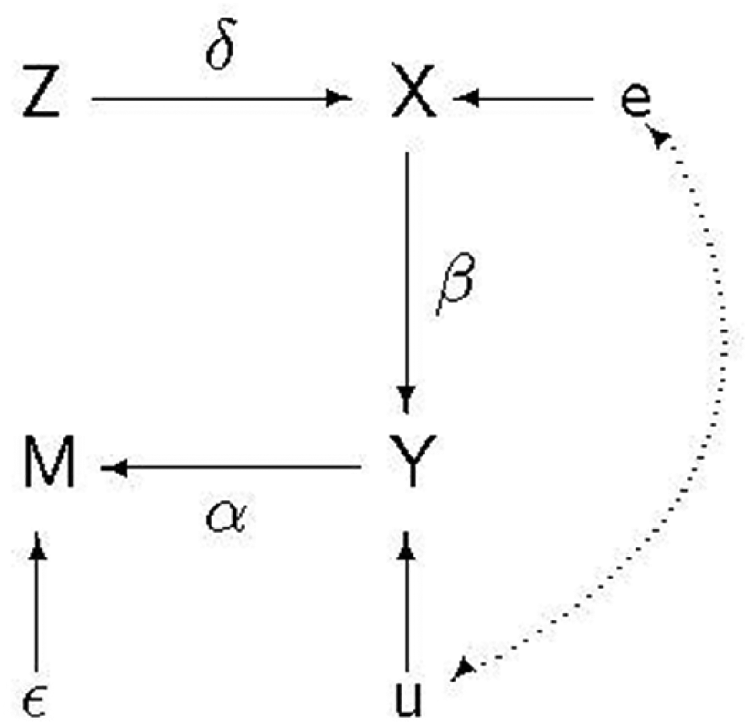
Colliders play a very important role in DAGs. A collider is a node in a graph that has more than one arrow going into it: in Figure 1, R is a collider on the path linking P and Q. A collider blocks a path on which it sits: so, according to this DAG, P and Q are independent. But conditioning on a collider opens the path: conditional on R, P and Q are no longer independent. Conditioning on a post-outcome collider arises when the data used are selected depending on their values of the outcome variable, Y. This may happen directly, as part of the design of the study or through decisions made about the analysis, or it may happen indirectly, through selecting data according to its values on a non-outcome variable which induces selection on the outcome. A common reason for conditioning on a post-outcome collider is missing data: people with low values of Y might have been less likely to report their value of Y in an interview or there may be missing values of a predictor of Y, say X, and so the pairs (X,Y) will be absent from the analysis when X is missing.

Figure 1.
A collider.

The layout of our paper is shown in Table 1. We consider five cases¹ corresponding to examples presented by E&W, with different mechanisms for determining whether data are observed or not and which variables, X and/or Y, are partially, rather than fully, observed as a result. We give an example of each case for expositional purposes. We treat our first case as canonical since it is the most general, and discussions of the later cases refer back to it. We consider a single outcome, Y, and a single predictor, X, but it is straightforward to generalize to more predictors. At the end of the paper, prompted by a reviewer's comment, we have included a short section in which we show how, under certain circumstances, IPW can be combined with instrumental variables estimation to overcome combined post-outcome collider bias and omitted variable bias in the relationship between X and Y.

Table 1.
The Cases we Consider.

Case E&W figure Missing is a function of Partially observed

1 6 X, Y X, Y

2 6 X, Y Y

3 5 Y Y

4 7 X, Y X, Y

5 6 Y X

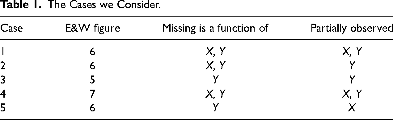
Case 1: Missing Data on X and Y: Complete Cases Analysis

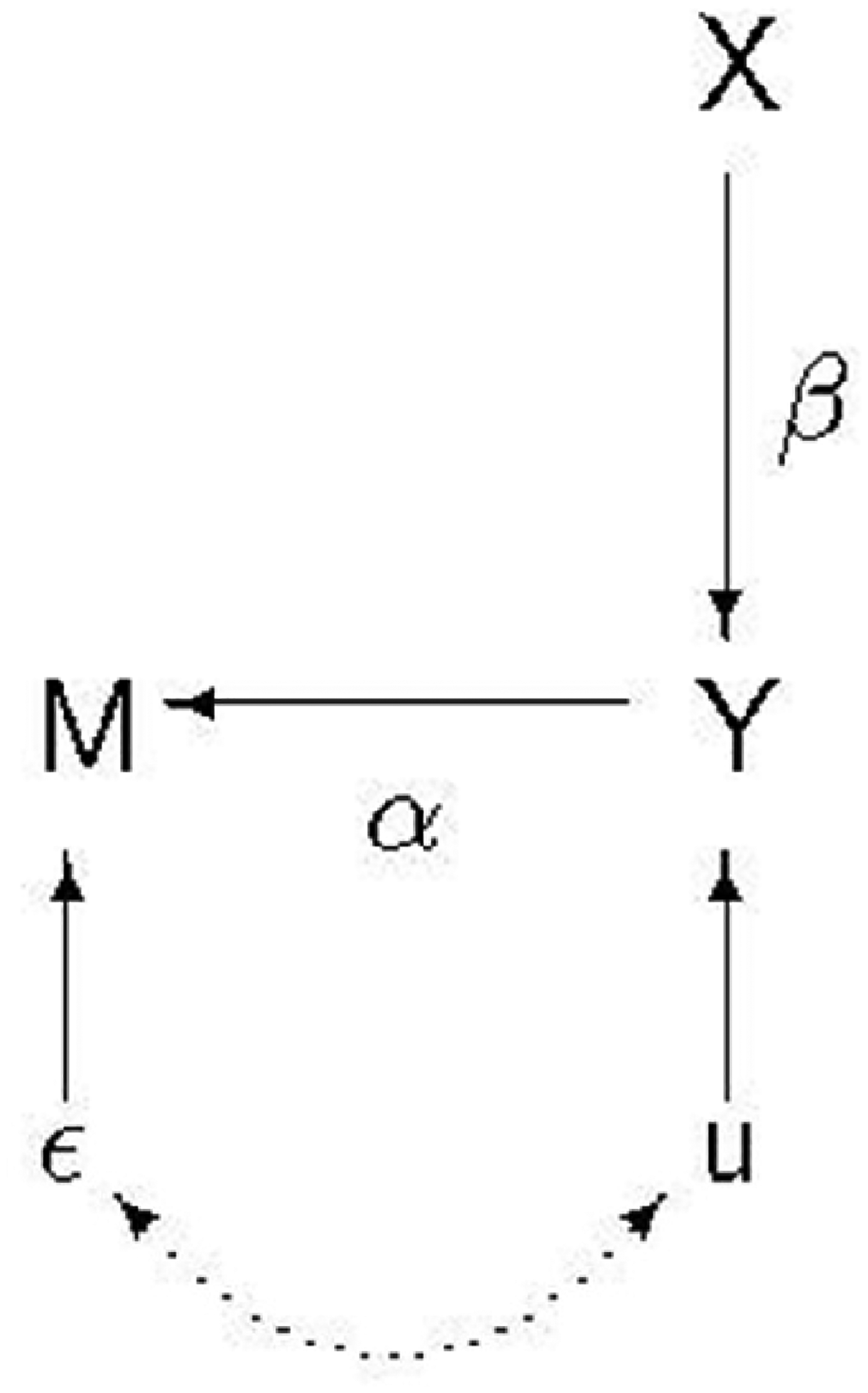
In Figure 2, X is a predictor of Y but whether or not we have data on both depends on X and Y. This duplicates Figure 6 of E&W (page 39). Unlike E&W we show the disturbance terms in the DAG: this will prove useful for explaining how collider bias arises. In E&W's example, we suppose we have data on a sample of divorced fathers and we want to know how their income, X, affects how much they pay in child support, Y. But some fathers do not respond to the study: M is a dummy variable indexing whether or not a father responds, and this depends both on a father's income and how much child support he pays.

Figure 2.
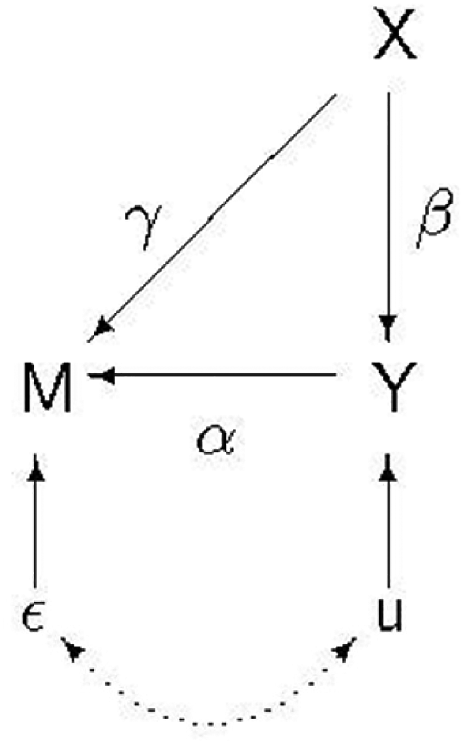
Post-outcome collider.

Linear models consistent with this DAG are
$Y = β X + u$
(1)
and, using the latent index formulation for a binary outcome,
$M^{} = α Y + γ X + ε$
(2)
and $M = 1 if M^{} > 0, M = 0$ otherwise, and $v a r (ε) = 1$ .

We assume $E (X u) = 0 = E (X ε)$ : in other words, there are no open backdoor paths from X to Y or from X to M, though we do not rule out paths from Y to M (which would be captured by $c o v (u, ε) \neq 0$ ). For ease of reference, we label the edges of the DAG in Figure 2 with the corresponding parameters from equations (1) and (2). We use a dashed line to show the possible association between the disturbances, u and $ε$ .

In our data we only observe cases for which 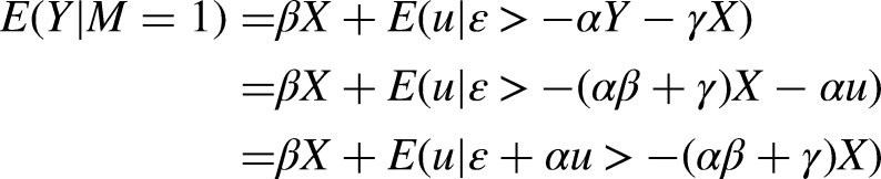$M = 1$ . The question then is whether OLS fitted to the observed data will produce unbiased estimates. In fact, OLS produces biased estimates of $β$ if either $α$ or $c o v (u, ε)$ is non-zero. The proof is as follows.
$\begin{aligned} E (Y | M = 1) = & β X + E (u | ε > - α Y - γ X) \\ = & β X + E (u | ε > - (α β + γ) X - α u) \\ = & β X + E (u | ε + α u > - (α β + γ) X) \end{aligned}$
Let $v = ε + α u, and v a r (v) = σ_{v}^{2}$ .² If v is normally distributed, $Φ (v / σ_{v})$ is the standard normal distribution function and $ϕ (v / σ_{v})$ is the standard normal density function. It follows from the statistics of truncated normal distributions that
$E (Y | M = 1) = β X + (\frac{σ_{u v}}{σ_{v}}) [\frac{ϕ (- ((α β + γ) X / σ_{v}))}{1 - Φ (- ((α β + γ) X / σ_{v}))}]$
(3)
$where σ_{u v} = c o v (u, v) = α E (u^{2}) + E (u ε) = α σ_{u}^{2} + c o v (u, ε) = α σ_{u}^{2} + σ_{u} ρ,$ where $ρ$ is the correlation coefficient between u and $ε$ .

The ratio in brackets is Heckman's “lambda” (Heckman 1979), or the inverse Mills ratio, which we denote as $λ ((α β + γ) X / σ_{v})$ . It is a monotone decreasing function of the probability that an observation is selected into the sample, $1 - Φ (- (α β + γ) X / σ_{v}) = Φ ((α β + γ) X / σ_{v})$ . It follows that if either $α$ or $ρ$ is non-zero, then OLS produces biased estimates of $β$ by confusing $β$ with how $λ ((α β + γ) X / σ_{v})$ varies with X (a selection effect). In Appendix 1, we illustrate this by showing how, in a specific case, $(σ_{u v} / σ_{v}) λ ((α β + γ) X / σ_{v})$ and the probability of selection, $Φ ((α β + γ) X / σ_{v})$ , vary with X and how the estimated marginal effect of X on Y varies with the probability of selection.

We can derive the sign of the bias in the OLS estimate of $β$ . If $α > 0, β > 0$ and $ρ \geq 0$ , the OLS estimator is downwardly biased because $σ_{u v} > 0$ , and thus $σ_{u v} λ ((α β + γ) X / σ_{v})$ declines with X. If $α σ_{u} < - ρ$ , then OLS is biased upwards. This follows because $σ_{u v} < 0$ in these circumstances and in this case $σ_{u v} λ ((α β + γ) X / σ_{v})$ increases with X. This is possible if, conditional on X, above average values of Y are associated with a lower chance of being in the sample $(ρ < 0)$ and the impact of Y on missingness $(α)$ or the variance of u $(σ_{u}^{2})$ is “small.” In our earlier example in which Y is child support payment and X is father's income, this might occur if the amount of child support paid had a small effect on being missing and those with unusually high child support payments were less likely to be in the sample.

We can use the DAG in Figure 2 to show, in a more general and intuitive way, how the bias arises when trying to estimate the effect of X on Y when conditioning on M. There are three biasing paths. Because M is a collider on the path from X to $ε$ we have the biasing path $X \to M \leftarrow ε \leftrightarrow u \to Y$ . M is also a collider on the path from X to Y and so we have the biasing path $X \to M \leftarrow Y$ . Furthermore, M is the descendant of a collider, Y, so we have the third biasing path $X \to u \to Y$ . If $c o v (ε, u) = 0$ the first path is zero and if $α = 0$ the second and third paths become zero, showing why OLS produces biased estimates of $β$ if either $α$ or $c o v (u, ε)$ is non-zero.

Inverse Probability Weighting

The IPW estimator weights the data by 1/ $p (Y, X)$ , where $p (Y, X)$ is the probability that $M = 1$ given Y and X. In the weighted data, M is independent of X and Y, and so X and Y have the same distribution when using only cases for which $M = 1$ as in the whole sample. In the case just considered, IPW is not available as a possible solution because IPW depends on having data on both Y and X to predict M and this is not possible when we only observe Y and X for observations in which $M = 1$ . If, however, we always observed either X or Y for everyone, then IPW would be a feasible estimator.

In order for IPW to produce a consistent estimate of a treatment effect, we need a conditional independence assumption (CIA), analogous to the propensity score theorem (Rosenbaum and Rubin 1983; see also Angrist and Pischke 2009:80). Suppose the treatment X is dichotomous and $Y_{0 i}$ and $Y_{1 i}$ are the potential outcomes for person i when $X_{i}$ = 0 and 1, respectively. Suppose the outcome Y (i.e., either $Y_{0 i}$ and $Y_{1 i}$ ) is observed for everyone. Let $M_{i} = 1$ indicate that we observe X for that person, $M_{i}$ = 0 otherwise. Define $p (Y_{i})$ as the probability that $M_{i} = 1$ conditional on $Y_{i}$ .

The CIA theorem states that:

If $[Y_{0 i}, Y_{1 i}]$ is orthogonal to $X_{i} | M_{i},$ then $[Y_{0 i}, Y_{1 i}]$ is orthogonal to $X_{i} | p (Y_{i})$ .

Now suppose that X is observed for everyone, but Y is not. Then, analogously, let $M_{i} = 1$ indicate that we observe Y for that person, $M_{i}$ = 0 otherwise. Define $p (X_{i})$ as the probability that $M_{i} = 1$ conditional on $X_{i}$ . The analogous CIA theorem states that:

If $[Y_{0 i}, Y_{1 i}]$ is orthogonal to $X_{i} | M_{i},$ then $[Y_{0 i}, Y_{1 i}]$ is orthogonal to $X_{i} | p (X_{i})$ .

There are three issues: (1) Can we assume that the CIA holds in these two special cases? (2) If so, can we obtain consistent estimates of $p (Y_{i})$ or $p (X_{i})$ ? (3) Is the IPW estimator an improvement on OLS?

Case 2: Missing Data on Y Only

Suppose that we have a situation in which there are missing values on Y but not on X; continuing the previous example, we suppose that all divorced men were interviewed and provided information about their income but some of them refused to answer the question about how much child support they pay. However, the naïve OLS model will still have to be fitted to data for which $M = 1$ and so the bias will be the same as in the first case as long as $α σ_{u} + ρ$ is non-zero.

IPW could be used here, however, because we have fully observed X and M. Our model to predict M would be
$M^{} = δ X + e$
(4)
and $M = 1 if M^{} > 0, M = 0$ otherwise.

But if the true missing data mechanism is as shown in equation (2), then $e = α Y + ε$ and $E (e Y) = α β^{2} E (X^{2}) + α σ_{u}^{2} + σ_{u} ρ \neq 0$ . A sufficient condition for $E (e Y) = 0$ is $α = 0 = ρ$ , but if this condition is satisfied, OLS would also yield a consistent estimator because, in that case, $σ_{u v} = 0$ in equation (3). It would take a particular set of parameters to satisfy $α β^{2} E (X) + α σ_{u}^{2} + σ_{u} ρ = 0$ when $α$ or $ρ$ are non-zero. For example, even if $α = 0$ , as in equation (4), we would need $ρ = 0$ . Thus, IPW applied to equation (1) fitted to cases for which $M = 1$ (as defined in equation (4)) would generally not be an improvement over unweighted OLS.

Case 3: Truncation of Y

A superficially similar situation to case 2 is when Y is observed only if it exceeds or falls below a particular value. An example of this is E&W's Figure 5. E&W's example concerns education, X, affecting income, Y, but the sample contains only people with low incomes 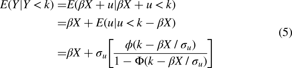$Y < k$ with k being some value of Y. Assuming that equation (1) generated the data, we find that (assuming u is normally distributed)
$\begin{aligned} E (Y | Y < k) = & E (β X + u | β X + u < k) \\ = & β X + E (u | u < k - β X) \\ = & β X + σ_{u} [\frac{ϕ (k - β X / σ_{u})}{1 - Φ (k - β X / σ_{u})}] \end{aligned}$
(5)
The second term on the right-hand side of (5) is once again related to the bias in the OLS estimator of $β$ applied to the observed data: in this case the bias is downward. As with case 1, because we lack any observations where $Y \geq k$ we cannot implement IPW. But if we knew the values of X for cases where $Y \geq k$ , even though we did not know their values of Y, and if we were willing to make a distributional assumption about u (e.g., that u is Normally distributed) we could use a censored regression, such as a Tobit model with an upper limit k in this example.³ Conditional on the assumed normality of u, maximum likelihood estimation of the model generates consistent estimates of $β$ and $σ_{u}$ , while OLS does not, as is well known.

Case 4: Ascertainment Bias

E&W Figure 7 (page 40) shows an example of ascertainment bias (Rothman, Greenland, and Lash 2008), and Figure 2 of this paper applies here too. In E&W's exposition, X is the commercial success of an album measured by whether it topped the Billboard charts, and Y is whether the album was included in the Rolling Stone 500. The sample of 1,700 albums on which the analysis (Schmutz 2005) was carried out was formed by selecting all albums in the Rolling Stone 500 and 1,200 other albums “all of which had earned some other elite distinction, such as topping the Billboard charts or winning a critics’ poll. Among the tens of thousands of albums released in the United States over the decades, the 1,700 sampled albums clearly represent a subset that is heavily selected for success.” (Elwert and Winship 2014:40).

Here the model of equations (1) and (2) applies with the minor change that Y is now binary (inclusion in the Rolling Stone 500 or not). So, in place of equation (1) we could write the latent variable model: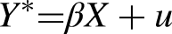
$Y^{} = β X + u$
with $Y = 1 if Y^{} > 0, 0$ otherwise. With this modification all the results for case 1 apply to this example too. They can also be used to suggest why Schmutz (2005) found a negative effect of X (topping the Billboard charts) on Y (being included in the Rolling Stone 500).

In our case 1, if $β$ = 0.1, $α = 0.5$ , $ρ = 0.2$ , and $γ = 0.5$ , we obtain negative values for dY/dX for most of the range of X, and so averaging over X in the data will yield a negative value for the OLS estimate. Although the details of how X is distributed could lead to other results, a negative estimate is very likely with these parameters. For example, if X has a uniform or symmetric distribution, the OLS estimate of $β$ is −0.06, even though $β$ = 0.1.

Case 5: Missing Data on X Only and M Independent of X

A situation in which there is collider bias but IPW can correct for it to yield unbiased estimates is shown in Figure 3. The difference between this and Figure 2 is that M is no longer affected by X and so we have
$M^{} = α Y + ε$
(6)
and $M = 1 if M^{} > 0, M = 0$ otherwise, and $v a r (ε) = 1$ .

Figure 3.
Selection on the outcome.

One situation in which this set-up will arise is in the use of survey data, where, although respondents provide information on an outcome (such as their own years of education), whether or not they respond to a question concerning a determinant of the outcome may depend on their outcome: for example, respondents with more years of education might be more likely to provide information about their own parents’ education. This is a particular example of a more widespread problem: studies of status attainment and inter-generational mobility almost always rely on respondents’ reports of their social origins (measured by parental occupation, and/or education) and whether or not this information is collected may depend on respondents’ own status (or class destination). Ignoring this is likely to lead to bias in estimates of intergenerational associations.

In this case, OLS will once again yield biased estimates, but $M *$ is now not affected by X and so, in equation (3), $γ = 0$ . We have
$E (Y | M = 1) = β X + (\frac{σ_{u v}}{σ_{v}}) [\frac{ϕ (- (α β X / σ_{v}))}{1 - Φ (- (α β X / σ_{v}))}]$
(7)
If $α > 0 & β > 0$ , then using only observations for which X is known over-represents the “top” part of both distributions to estimate $β$ . As before, and recalling that $σ_{u v} = α σ_{u}^{2} + σ_{u} ρ$ , if either $α$ or $ρ$ is non-zero OLS using only the observations for which M = 1 produces biased estimates of $β$ by confusing the variation in the inverse Mills ratio, $λ (α β X / σ_{v})$ with the estimate of $β$ . Figure 3 shows why this bias arises. By conditioning on M we are conditioning on the descendant of a collider (Y in this case) and this has the same consequence as conditioning on Y itself, namely, opening a path from X to u to Y.

In this case, however, IPW can be used under certain conditions. In the model to predict missingness, based on equation (6) above, we require that the estimate of $α$ is consistent, and this requires $E (ε Y) = 0$ . Expanding this we have
$E (ε Y) = E (ε (β X + u)) = c o v (u, ε) = σ_{u} ρ$
(8)
We therefore require that $ρ = 0$ ; in other words, $E (ε u) = 0$ This requirement is necessary because IPW estimation conditions only on observables. It is, however, a weaker assumption than is needed for OLS to be unbiased (where we also require $α = 0$ ).

Bareinboim, Tian and Pearl (2014) address problems of selection bias using a graphical, non-parametric approach with the goal of recovering the probability of an outcome, Y, conditional on one or more predictors, X in the face of sample selection.⁴ Their approach is more general than ours and so our results for cases 1 and 2, for example, are special cases of results they demonstrate. For our case 5, we are able to recover the conditional mean $E (Y | X)$ but Bareinboim et al. (2014) show that, in such a situation, one cannot recover the full conditional distribution of Y given X.

Monte Carlo Simulations

Table 2 shows the OLS estimates using simulated data generated according to equations (1) and (2). Each simulation assumes that X is a standard normal variable uncorrelated with $u and ε$ , and $[u, ε]$ is joint standard normal with correlation coefficient $ρ$ . The simulations vary $γ$ and the correlation between u and $ε$ while keeping the parameter values for $α$ and $β$ fixed. As can be seen, OLS is biased even when $ρ = 0$ and $γ = 0$ . The bias is downward and it increases as $ρ$ increases.

Table 2.
Comparison of Simulated OLS and IPW Estimates of $β$ : $α = 0.5 and β = 0.5$ (SD in Parentheses).

$ρ = 0$ $ρ = - 0.2$ $ρ = 0.2$

$γ$ OLS IPW OLS IPW OLS IPW

0 0.438 (0.021) 0.499 (0.032) 0.455 (0.022) 0.488 (0.026) 0.424 (0.020) 0.522 (0.043)

0.1 0.414 (0.022) 0.480 (0.036) 0.439 (0.022) 0.477 (0.028) 0.395 (0.021) 0.496 (0.049)

0.2 0.392 (0.022) 0.460 (0.039) 0.424 (0.023) 0.466 (0.030) 0.368 (0.021) 0.469 (0.056)

0.3 0.372 (0.023) 0.440 (0.042) 0.409 (0.024) 0.455 (0.032) 0.343 (0.022) 0.439 (0.069)

0.4 0.353 (0.023) 0.420 (0.045) 0.397 (0.024) 0.445 (0.034) 0.319 (0.022) 0.407 (0,070)

0.5 0.336 (0.024) 0.400 (0.048) 0.386 (0.025) 0.435 (0.036) 0.298 (0.023) 0.373 (0.074)

N = 4,000, 2,000 replications, X is a standard normal variable uncorrelated with $u and ε$ , and $[u, ε]$ is joint standard normal with correlation coefficient $ρ$ . Data is generated using equations (1) and (2). Simulations vary $γ$ and the correlation between u and $ε$ while keeping the parameter values for $α$ and $β$ fixed.

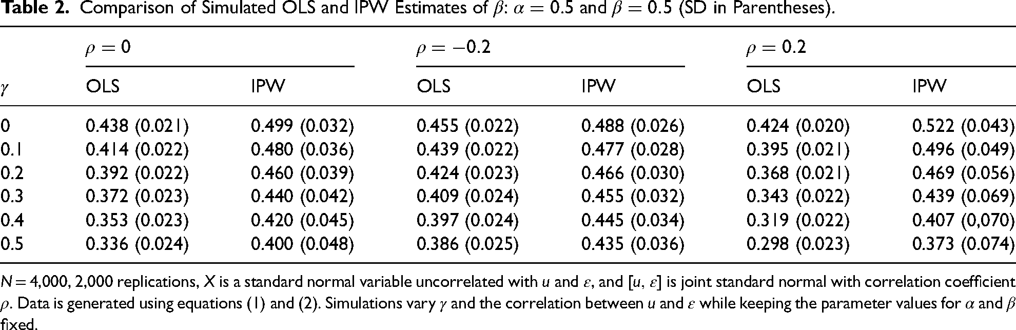
Table 2 indicates that, at least in the parameter configurations illustrated, when the condition $ρ = 0$ and $γ = 0$ is not satisfied the IPW estimates are closer to the true value of $β$ than the OLS estimates. Also, comparisons between the $ρ = 0 and ρ = 0.2$ panels suggest that, for a given $ρ$ , the omission of X in the computed weight equation operates to reduce the estimate of $β$ while $ρ > 0$ operates in the opposite direction. When $ρ < 0$ , the IPW estimate is always biased downward, but closer to the true value than the OLS estimate.

Table 3 illustrates how the IPW estimates of $β$ vary with a wider range of $γ and ρ$ . Most IPW estimates are below the true value, the exception being when $γ$ is relatively small and $ρ > 0$ and relatively large (e.g., when $γ = 0.1$ , $ρ > 0.2$ ).

Table 3.
Variation in IPW Estimates of $β$ by $γ and ρ$ : $α = 0.5 and β = 0.5$ (Estimates Below the True Value in Bold).

$γ$ $ρ$

−0.2 −0.1 0 0.1 0.2 0.3 0.4 0.5

0 0.488 0.492 0.499 0.509 0.533 0.537 0.556 0.575

0.1 0.477 0.476 0.480 0.487 0.496 0.507 0.522 0.537

0.2 0.466 0.461 0.460 0.463 0.469 0.476 0.485 0.494

0.3 0.455 0.446 0.440 0.438 0.439 0.441 0.442 0.449

0.4 0.445 0.431 0.420 0.412 0.407 0.403 0.399 0.395

0.5 0.435 0.416 0.400 0.386 0.373 0.363 0.353 0.338

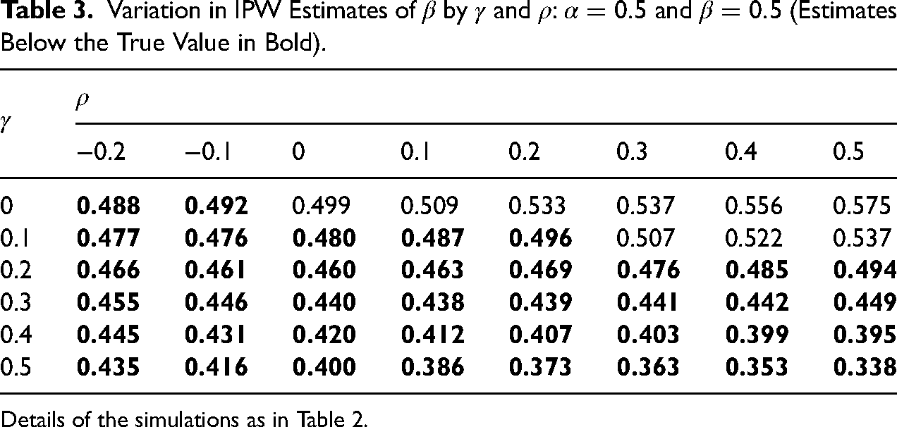
Details of the simulations as in Table 2.

However, there are constellations of parameters in our model setup in which OLS produces unbiased estimates. This would happen for non-zero $α$ if $σ_{u v} = 0$ , or equivalently, when $α σ_{u} = - ρ$ , which requires $ρ < 0$ . For instance, with the parameters $α = 0.5 = β and σ_{u} = 1$ , this requires $ρ = - 0.5$ . A Monte Carlo simulation of the model with these parameters confirms that the OLS estimator of $β$ is unbiased and consistent (the estimate is 0.500, s.e. = 0.023), and the IPW estimate is close to it: 0.504 (0.023), despite the fact that the estimate of $α$ from the probit selection equation is inconsistent because $ρ < 0$ .

With $ρ = 0$ and $γ = 0$ IPW returns an unbiased and consistent estimate of the regression coefficients. As Table 3 shows, as $ρ$ deviates from zero, the IPW estimates become biased, but this bias is generally small, with the 95% confidence interval (not reported in the table) including the true value, at least for $| ρ | \leq 0.2$ , suggesting the estimates are robust to some degree of correlation between the error terms of the two equations. Even low to moderate values of $γ$ (e.g., $γ \leq 0.2$ ) produce estimates of $β$ close to its true value and certainly closer to it than OLS. Appendix 2 shows how the computed weights that impose $γ = 0$ differ from the true weights for different values of $γ$ and $ρ$ . The analysis suggests that IPW based on $w_{C} = 1 / Φ (\hat{α} Y)$ rather than the true weight of $1 / Φ (α Y + γ X)$ does not do a bad job in mimicking the true weight as long as $ρ = 0$ , even when the parameter on the omitted X variable is relatively large. But when $| ρ | > 0$ , its performance is much poorer.

We conclude that the types of collider bias considered imply inconsistent OLS estimation of linear models. But the simple IPW estimator appears to do better than OLS in the case when selection depends on Y only, and under some plausible parameter restrictions the estimates of $β$ can be close to the true value of $β$ . Practitioners are advised to report both OLS and IPW estimates when there is concern about sample selection based on the dependent variable. There are a number of important applications in which such selection might be plausible, and the next section considers one such application.⁵

An Illustration: Intergenerational Transmission of Education

We use data from the British Household Panel Study (BHPS) to estimate the effects of parents’ education on the educational attainment of their adult (respondent) children. In the BHPS information on parents’ highest education level was not collected until wave 13 (2003). Evidence indicates that people with higher education are less likely to leave the panel (lower attrition), suggesting that respondents with higher education are more likely to be observed and to provide data on parents’ education, which is indeed confirmed by the BHPS data.⁶ Because it is the respondent who is making the decision about continuing participation in the panel, IPW estimation of a selection model based solely on the respondent's own education may perform quite well because, in terms of the parameters of equations (1) and (2), $α$ is large relative to $γ$ , so, even if we do not obtain a consistent estimate of $α$ in equation (1), the estimated equation may still work well in computing the propensity score (see Appendix 2).

For easier comparability between generations, we focus on a simple binary indicator of highest education: whether a person has a university degree or not. Among 4,369 persons born during 1955–85, 19.7% obtained a degree, and among those for which we observed father's education (2,672), 10% of fathers had a degree. The analogous statistics for mother's education are 2,745 observed with 6.7% of mothers having obtained a degree. Thus, father's (mother's) education is observed for 61% (70%) of the sample.

In the models we estimate we also allow the probability of sample selection and child's education to depend on year of birth and sex, which are observed for everyone. In Table 4, only the coefficients associated with education are reported. The first two models estimate the parameters for one or other of the parent's education on its own; a third estimates separate parameters for each parent's education using the selected sample in which both parents’ education is observed. The coefficients in the selection model are from a probit model and those in the intergenerational education equation are from a linear model.

Table 4.
Estimates of the Intergenerational Education Equation^a.

(A) Father's education model

Coef. Std. Err. 95% Conf. interval

Selection equation

Child degree 0.525 0.052 0.42 0.63

Education equation

OLS, father degree 0.380 0.027 0.33 0.43

IPW, father degree 0.353 0.032 0.29 0.42

(B) Mother's education model

Coef. Std. Err. 95% Conf. interval

Selection equation

Child degree 0.370 0.053 0.27 0.47

Education equation

OLS, mother degree 0.325 0.032 0.26 0.39

IPW, mother degree 0.297 0.037 0.22 0.37

(C) Both parents’ education model

Coef. Std. Err. 95% Conf. interval

Selection equation

Child degree 0.525 0.052 0.42 0.63

Education equation

OLS

Mother degree 0.174 0.035 0.10 0.24

Father degree 0.317 0.030 0.26 0.37

IPW

Mother degree 0.161 0.040 0.08 0.24

Father degree 0.296 0.035 0.23 0.36

^a
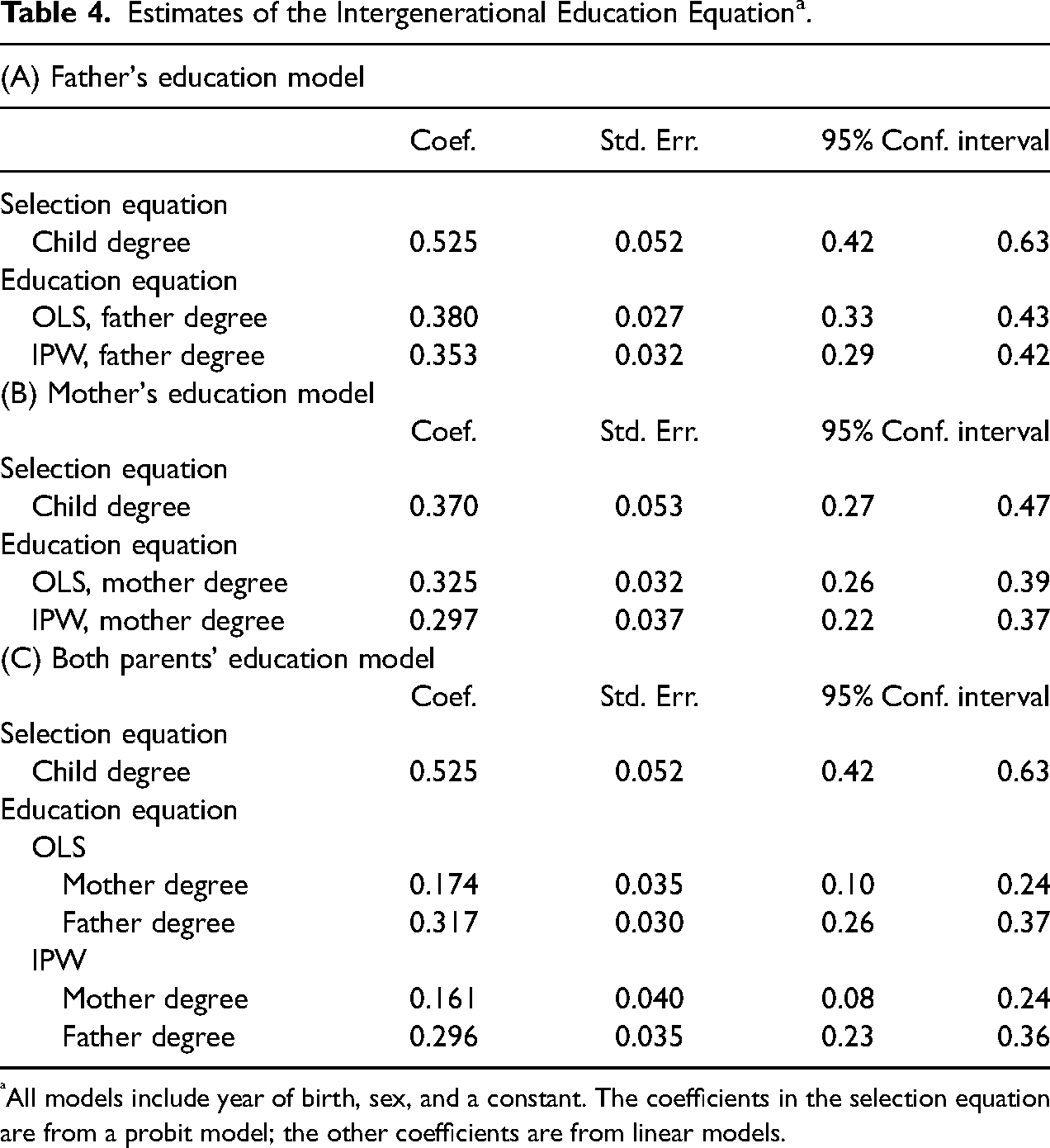
All models include year of birth, sex, and a constant. The coefficients in the selection equation are from a probit model; the other coefficients are from linear models.

Table 4 indicates that, in all models, the IPW estimates of the parents’ education coefficient are below the OLS ones, but generally close to them, as judged by the confidence intervals of each. This could happen because $ρ < 0$ and is sufficiently large in magnitude. For example, consider a model similar in structure to equations (1) and (2) except that both X and Y are dichotomous and driven by latent variables for each in which $α = 0.5, γ = 0 and β = 0.5$ . A Monte Carlo simulation of that model (N = 4,000, replications = 2,000) in which $ρ = - 0.4$ yields an OLS estimate of 0.193 (SD = 0.02) and an IPW estimate of 0.190 (SD = 0.02). Similar differences emerge when $γ = 0.2$ (OLS and IPW estimates of 0.196 and 0.195, respectively). In keeping with the dichotomous nature of the generated data, a probit model may seem more appropriate, but similar results emerge: the IPW and conventional probit estimates of $β$ are 0.496 (SD = 0.052) and 0.498 (SD = 0.052) when $γ = 0$ , and 0.507 (SD = 0.051) and 0.508 (SD = 0.051) when $γ = 0.2$ .⁷

Combining IV and IPW

In Case 5 and the DAG shown in Figure 3, the crucial assumption that allows us to overcome post-outcome collider bias is $E (ε u) = 0$ : the disturbances for Y and M are independent. But there are two further assumptions about disturbances that we maintained throughout: $E (X u) = 0$ and $E (X ε) = 0$ . The first rules out open backdoor paths from X to Y, the second rules out open backdoor paths from X to M. In this section, we show that if the first assumption does not hold (in which case we have “omitted variable bias”) we can still estimate the effect of X on Y consistently, even in the presence of post-outcome collider bias, provided we have a suitable instrumental variable. In other words, instrumental variables and IPW can be combined to deal with simultaneous omitted variable bias and post-outcome collider bias.

We write the first stage of the IV estimator as
$X = δ Z + e$
(9)
where E(eZ) = 0, and the reduced form as
$Y = θ Z + u$
(10)
The DAG in question is shown in Figure 4. There is no path directly linking the disturbances u and $ε$ : this assumption is necessary for what follows. We assume the effect of X on Y is homogeneous (so we are not estimating a local average treatment effect) and that Z is an IV that meets the criteria of instrument relevance and instrument validity (i.e., $E (Z u) = 0$ ). We assume, initially, that Z is observed for all cases. The dashed line in Figure 4 shows a correlation between the disturbances e and u ( $E (e u) \neq 0$ ) which is why we need an instrument. We assume $E (e ε) = 0$ (this is a rewriting of our assumption $E (X ε) = 0$ ), and $E (e Z) = 0$ , so estimating (9) by OLS would yield an unbiased estimate, $\hat{δ}$ . Because Y and Z are fully observed, the OLS estimate, $\hat{θ}$ , is unbiased and ${\hat{β}}_{I V} = \hat{θ} / \hat{δ}$ is a consistent estimator of the effect of X on Y, $β .$

Figure 4.
Omitted variable bias and conditioning on a post-outcome collider.

But we cannot estimate (9) because X is only observed when 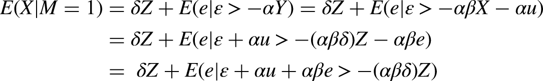$M = 1$ . Then we have
$\begin{aligned} E (X | M = 1) & = δ Z + E (e | ε > - α Y) = δ Z + E (e | ε > - α β X - α u) \\ = δ Z + E (e | ε + α u > - (α β δ) Z - α β e) \\ = δ Z + E (e | ε + α u + α β e > - (α β δ) Z) \end{aligned}$
Let $w = ε + α u + α β e, and v a r (w) = 1 + (α β)^{2} v a r (e) + α^{2} σ_{u}^{2} + 2 α c o v (ε, u) + 2 α^{2} β c o v (e, u) = σ_{w}^{2}$
$E (X | M = 1) = δ Z + (\frac{σ_{e w}}{σ_{w}}) [\frac{ϕ (- (α β Z / σ_{w}))}{1 - Φ (- (α β Z / σ_{w}))}]$
(11)
where $σ_{e w} = α c o v (e, u) + α β v a r (e)$ .

The second term on the RHS of (11) is the bias from using OLS, which then transfers to the IV estimator making it inconsistent. However, just as, in our fifth case, we could use IPW to estimate $β$ , so we can use IPW here to estimate $δ$ when $E (u ε) = 0$ . The selection process is the same in both cases (with M depending only on Y) and we can estimate it unbiasedly.

Indeed, because in this example M depends only on Y, we do not require that Z is fully observed. Assuming we only observe Z when $M = 1$ clearly does not affect our estimate of $δ$ and we can correctly estimate $θ$ using only data for which $M = 1$ via IPW. The intuition here is that, if we substitute X for Z, this is the same model as we considered in Case 5.

Conclusions

Conditioning on a post-outcome collider is not an uncommon occurrence in the social sciences. Elwert and Winship (2014) presented a number of examples to illustrate the problems that can arise. We have built on their work but we have also investigated possible solutions. Using linear models, we have derived expressions for the bias arising in different kinds of conditioning on a post-outcome collider, we have shown how the biases arise, and we have explained the specific situations in which IPW will allow us to obtain estimates that are either consistent or, if not consistent, then less biased than those from OLS regressions.

Case	E&W figure	Missing is a function of	Partially observed
1	6	X, Y	X, Y
2	6	X, Y	Y
3	5	Y	Y
4	7	X, Y	X, Y
5	6	Y	X

	$ρ = 0$	$ρ = - 0.2$	$ρ = 0.2$
0	0.438 (0.021)	0.499 (0.032)	0.455 (0.022)	0.488 (0.026)	0.424 (0.020)	0.522 (0.043)
0.1	0.414 (0.022)	0.480 (0.036)	0.439 (0.022)	0.477 (0.028)	0.395 (0.021)	0.496 (0.049)
0.2	0.392 (0.022)	0.460 (0.039)	0.424 (0.023)	0.466 (0.030)	0.368 (0.021)	0.469 (0.056)
0.3	0.372 (0.023)	0.440 (0.042)	0.409 (0.024)	0.455 (0.032)	0.343 (0.022)	0.439 (0.069)
0.4	0.353 (0.023)	0.420 (0.045)	0.397 (0.024)	0.445 (0.034)	0.319 (0.022)	0.407 (0,070)
0.5	0.336 (0.024)	0.400 (0.048)	0.386 (0.025)	0.435 (0.036)	0.298 (0.023)	0.373 (0.074)

$γ$	$ρ$
0	0.488	0.492	0.499	0.509	0.533	0.537	0.556	0.575
0.1	0.477	0.476	0.480	0.487	0.496	0.507	0.522	0.537
0.2	0.466	0.461	0.460	0.463	0.469	0.476	0.485	0.494
0.3	0.455	0.446	0.440	0.438	0.439	0.441	0.442	0.449
0.4	0.445	0.431	0.420	0.412	0.407	0.403	0.399	0.395
0.5	0.435	0.416	0.400	0.386	0.373	0.363	0.353	0.338

(A) Father's education model
Selection equation
Child degree	0.525	0.052	0.42	0.63
Education equation
OLS, father degree	0.380	0.027	0.33	0.43
IPW, father degree	0.353	0.032	0.29	0.42
(B) Mother's education model
	Coef.	Std. Err.	95% Conf. interval
Selection equation
Child degree	0.370	0.053	0.27	0.47
Education equation
OLS, mother degree	0.325	0.032	0.26	0.39
IPW, mother degree	0.297	0.037	0.22	0.37
(C) Both parents’ education model
	Coef.	Std. Err.	95% Conf. interval
Selection equation
Child degree	0.525	0.052	0.42	0.63
Education equation
OLS
Mother degree	0.174	0.035	0.10	0.24
Father degree	0.317	0.030	0.26	0.37
IPW
Mother degree	0.161	0.040	0.08	0.24
Father degree	0.296	0.035	0.23	0.36

Footnotes

Acknowledgements

We are grateful for helpful comments from two reviewers and the editor.

Declaration of Conflicting Interests

The authors declared no potential conflicts of interest with respect to the research, authorship, and/or publication of this article.

Funding

The authors disclosed receipt of the following financial support for the research, authorship, and/or publication of this article: John Ermisch's contribution to the work was funded by a Leverhulme Trust Grant for the Leverhulme Centre for Demographic Science, University of Oxford.

ORCID iD

Richard Breen

John Ermisch

Notes

Author Biographies

Richard Breen is Professor of Sociology and Fellow of Nuffield College, University of Oxford. His research interests are inequality, intergenerational mobility, and quantitative methods. His recent publications have appeared in Annual Review of Sociology, Demography, and European Sociological Review. Together with Walter Müller he edited Education and Intergenerational Social Mobility in Europe and the United States (Stanford University Press, 2020). He is a Fellow of the British Academy and a Member of the Royal Irish Academy.

John Ermisch is emeritus professor of family demography at the University of Oxford, a senior research fellow at Nuffield College, a Fellow of the British Academy (since 1995) and an associate of the Leverhulme Centre for Demographic Science. He is the author of An Economic Analysis of the Family (Princeton University Press, 2003), Lone Parenthood: An Economic Analysis (Cambridge University Press, 1991) and The Political Economy of Demographic Change (Heinemann, 1983), as well as numerous articles in economic and demographic journals. More recently, he is co-editor of From Parents to Children: The Intergenerational Transmission of Advantage (New York: Russell Sage Foundation, 2012). He is Editor in Chief of Population Studies.

Appendix 1: Bias and the Probability of Selection

Figure A1 illustrates how $(σ_{u v} / σ_{v}) λ ((α β + γ) X / σ_{v})$ and the probability of selection, $Φ ((α β + γ) X / σ_{v})$ , vary with X when the parameters are set at $α = 0.5, β = 0.5,$ $γ = 0 and ρ = 0$ . $λ ((α β + γ) X / σ_{v})$ declines as the probability of selection increases. The conditional mean $E (Y | M = 1)$ is a non-linear function of X when $σ_{u v}$ is not zero. Thus, the marginal effect of X on it is not $β$ , but rather $β$ plus the derivative of $σ_{u v} λ$ with respect to X, which we denote $d y / d x$ .

Using the same parameter values, Figure A2 illustrates how $d y / d x$ varies with the probability of selection and also the downward bias of OLS. If $σ_{u v}$ = 0, (which, with the other parameter assumptions implies $α = 0$ ), $d y / d x$ would be a flat line at $β = 0.5$ and $Φ ((α β + γ) X / σ_{v})$ would equal 0.5. $d y / d x$ increases toward 0.5 as the probability of selection increases.

Appendix 2: IPW Weights: Bias and Covariation With True Weights

The true weights are given by $w_{T} = 1 / Φ (α Y + γ X)$ . Given that we cannot observe X, we compute the weights from a probit regression with Y as the only explanatory variable: $w_{C} = 1 / Φ (\hat{α} Y)$ . Form the ratio $r_{w} = w_{C} / w_{T}$ . Bias will be indicated by a mean ratio different from unity. Table A1 shows simulated mean values for $r_{w}$ for different values of $γ$ and $ρ$ , the correlation coefficient between $ε$ and u.

Table A1 indicates that $r_{w}$ is unbiased when $ρ = 0$ , but when $ρ = 0.2$ , the computed weight exceeds the true weight by 10% on average. Bias would not be an issue if $r_{w}$ were similar across observations, but it exhibits larger variance when $ρ = 0.2$ and when $γ$ is larger.

Table A2 examines the same issue in a different way by looking at the correlation between the computed and true weights. It shows that when $ρ = 0$ , the correlation of the computed and true weights is relatively high, although it declines as the parameter on the omitted X variable, $γ$ , increases. But when $ρ = 0.2$ , the mean correlation declines substantially, with even its maximum value being below unity.

These simulations suggest that IPW based on $w_{C} = 1 / Φ (\hat{α} Y)$ does not do a bad job in mimicking the true PS weight as long as $ρ = 0$ , even when the parameter on the omitted X variable is relatively large. But when $ρ > 0$ , its performance is much poorer.

References

Angrist, Joshua D. & Jörn-Steffen Pischke. 2009. Mostly Harmless Econometrics: An Empiricist's Companion. Princeton University Press.

Bareinboim

Elias

Pearl

Judea

. 2016. “Causal Inference and the Data Fusion Problem.” Proceedings of the National Academy of Sciences 113:7345-52.

Bareinboim

Elias

Tian

Jin

Pearl

Judea

. 2014. “Recovering From Selection Bias in Causal and Statistical Inference.” Pp. 2410-6 in Proceedings of the Twenty-Eighth AAAI Conference on Artificial Intelligence.

Breen

Richard

. 2018. “Some Methodological Problems in the Study of Multigenerational Mobility.” European Sociological Review 34:603-11.

Elwert

Felix

Winship

Christopher

. 2014. “Endogenous Selection Bias: The Problem of Conditioning on a Collider Variable.” Annual Review of Sociology 40:31-53.

Heckman

James J.

1979. “Selection Bias as a Specification Error.” Econometrica 47:153-61.

Horvitz

D. G.

Thompson

D. J.

. 1952. “A Generalization of Sampling Without Replacement from a Finite Universe.” Journal of the American Statistical Association 47:663-85.

Lawrence

Matthew

Breen

Richard

. 2016. “And Their Children After Them? The Effect of College on Educational Reproduction.” American Journal of Sociology 122:532-72.

Mohan

Karthika

Pearl

Judea

. 2019. Graphical Models for Processing Missing Data. arXiv:1801.03583v2.

10.

Pearl

Judea

. 2013. “Linear Models: A Useful “Microscope” for Causal Analysis.” Journal of Causal Inference 1:155-70.

11.

Rosenbaum, Paul R. & Donald B. Rubin. 1983. “The Central Role of the Propensity Score in Observational Studies for Causal Effects.” Biometrika 70: 41–55.

12.

Rothman

K. J.

Greenland

Lash

T. L.

. 2008. “Case-control Studies.” Pp. 111-27 in Modern Epidemiology, 3rd ed., edited by Rothman

K. J.

Greenland

Lash

T. L.

. Philadelphia, PA: Lippincott.

13.

Seaman

Shaun R.

White

Ian R.

. 2011. “Review of Inverse Probability Weighting for Dealing with Missing Data.” Statistical Methods in Medical Research 22(3):278-95.

14.

Schmutz

2005. “Retrospective Cultural Consecration in Popular Music.” American Behavioral Scientist 48:1510-23.

15.

Sharkey

Patrick

Elwert

Felix

. 2011. “The Legacy of Disadvantage: Multigenerational Neighborhood Effects on Cognitive Ability.” American Journal of Sociology 116:1934-81.

$γ$	$ρ$
	−0.2	−0.1	0	0.1	0.2	0.3	0.4	0.5
0	0.488	0.492	0.499	0.509	0.533	0.537	0.556	0.575
0.1	0.477	0.476	0.480	0.487	0.496	0.507	0.522	0.537
0.2	0.466	0.461	0.460	0.463	0.469	0.476	0.485	0.494
0.3	0.455	0.446	0.440	0.438	0.439	0.441	0.442	0.449
0.4	0.445	0.431	0.420	0.412	0.407	0.403	0.399	0.395
0.5	0.435	0.416	0.400	0.386	0.373	0.363	0.353	0.338

Using Inverse Probability Weighting to Address Post-Outcome Collider Bias

Abstract

Keywords

Colliders and Conditioning on a Post-Outcome Collider

Case 1: Missing Data on X and Y: Complete Cases Analysis

Inverse Probability Weighting

Case 2: Missing Data on Y Only

Case 3: Truncation of Y

Case 4: Ascertainment Bias

Case 5: Missing Data on X Only and M Independent of X

Monte Carlo Simulations

An Illustration: Intergenerational Transmission of Education

Combining IV and IPW

Conclusions

Footnotes

Acknowledgements

Declaration of Conflicting Interests

Funding

ORCID iD

Notes

Author Biographies

Appendix 1: Bias and the Probability of Selection

Appendix 2: IPW Weights: Bias and Covariation With True Weights

References