
Abstract
Suppose X and Y are binary exposure and outcome variables, and we have full knowledge of the distribution of Y, given application of X. We are interested in assessing whether an outcome in some case is due to the exposure. This “probability of causation” is of interest in comparative historical analysis where scholars use process tracing approaches to learn about causes of outcomes for single units by observing events along a causal path. The probability of causation is typically not identified, but bounds can be placed on it. Here, we provide a full characterization of the bounds that can be achieved in the ideal case that X and Y are connected by a causal chain of complete mediators, and we know the probabilistic structure of the full chain. Our results are largely negative. We show that, even in these very favorable conditions, the gains from positive evidence on mediators is modest.
Keywords
Introduction
Even the best possible evidence regarding the effects of a treatment on an outcome in a population is generally not enough to identify the probability that a positive outcome in an individual treated case was in fact caused by the treatment.
For instance, researchers conducting randomized controlled trials may determine that providing a medicine to school children increases the overall probability of good health from one third to two thirds. This information, no matter how precise, is not enough to answer the following question: Is Ann healthy because she took the medicine? It is not even enough to answer the question probabilistically. The reason is that, consistent with these results, it may be that the medicine makes a positive change for two out of three children, but a negative change for the remainder: In that case, the medicine certainly helped Ann. But it might alternatively be that the medicine makes a positive change for one in three children but no change for the others. In that case, the chances it helped Ann are just one in two. For, of the children taking the medicine, two thirds are healthy. Half of these are healthy because of the medicine, whereas the other half would have been healthy anyway.
Put differently, the experimental data identifies the “effects of causes,” but we are interested in the reverse problem, of quantifying “causes of effects.” The causes of effects task of defining and assessing the probability of causation (Robins and Greenland 1989) in an individual case have been considered by Tian and Pearl (2000); Dawid (2011); Yamamoto (2012); Pearl (2015); Dawid, Musio and Fienberg (2016); and Murtas, Dawid, and Musio (2017). 1 Note that this is distinct from the “reverse causal question” of Gelman and Imbens (2013), which is a collection of effects of causes questions aimed at ascertaining which causes have an effect on an outcome—the difference being that the estimand in this formulation does not condition on observed values of treatments and outcomes. The question is of interest for historical analyses that seek to explain outcomes, for judicial determinations of innocence or guilt, and policy analysis seeking to assign responsibility for outcomes to interventions. For these outcomes, bounds are useful when they are narrow—in which case they can be treated like point estimates despite the lack of identification. But even less narrow bounds can sometimes be useful and support claims of the form: For any possible priors you might hold you should conclude that Y was more likely than not due to X. Finally, knowing that bounds are not narrow is useful since it clarifies that claims about causal attribution reflect prior beliefs about causal processes and not beliefs justified by data. For all these cases, we highlight that determining that X caused Y does not in any way mean that X is the only cause of Y or the most important cause of Y. For this reason, the attribution question can be addressed without needing to take account of other possible causes—although, as we will show, taking account of these may sometimes sharpen conclusions.
A common approach to learning about causes of effects is to seek additional evidence along causal pathways. Observation of such ancillary evidence can then act like a test, leading to updating on overall causal relations. Using the language in Van Evera (1997), a “smoking gun test” searches for evidence that, though unlikely to be found, would give great confidence in a claim if it were to be found; a “hoop” test is a search for evidence that we expect to find, but which, if found to be absent, would provide compelling evidence against a proposition (as if the proposition were asked to jump through a hoop).
Though these tests do not require that causal process observations lie along a simple chain—what Weller and Barnes (2016) call scenario 1 chains and we call a chain with complete mediation—in many applications, researchers presume that they do. In the account provided in Mahoney (2012), Skocpol (1979) produced a hoop test by identifying a mediator M (local events) such that X (community solidarity) was necessary for M and M was sufficient for Y (peasant revolution). As described also by Mahoney (2012), researchers might use chains to justify smoking gun tests, seeking “chains of necessary conditions.” A common practice among researchers evaluating development programs is to specify “theories of change” and seek evidence for intermediate outcomes along a pathway linking treatment to outcomes (Ghate 2018): Was the treatment received? Was the medicine ingested? Knight and Winship (2013) review a long history in sociology of “mechanism-focused scholarship,” including in Max Weber, Karl Marx, and Paul Lazerfeld. Gross (2018) describes the many different classes of causal chains used in sociological research, many of which involve complete mediation (or linearity, to use his term).
This strategy of looking at values of a mediating variable is often extended by examining multiple points on a chain. Seeing supportive evidence at many points along such a causal chain would appear to give confidence that the final outcome is indeed due to the conjectured cause. This is a common idea in process tracing (Collier 2011) as well as of mixed methods research as used in development evaluation (White 2009). As described by Mahoney (2012), “[a]lthough a hypothesis that passes any one straw in the wind test may not be well supported, a hypothesis that passes several straw in the wind tests may generate a good deal of confidence in its validity.” In the most optimistic accounts of observation of causal chains, it is reasoned that, as one gets close enough to a process, by observing more and more links in a chain, the link between any two steps becomes less questionable—intuitively obvious—and eventually the causal process reveals itself (Mahoney 2012:581).
We here provide a comprehensive treatment of the scope for inferences of this form. Our analyses employs causal models for justifying mechanistic accounts as advocated by Knight and Winship (2013). The analysis builds on logic found in Mahoney (2012) by quantifying the learning that can be made from cases involving necessity and sufficiency as well as probabilistic relations. Whereas existing results (Dawid, Murtas, and Musio 2016) have considered the case of a single unobserved mediator, we generalize by considering situations with chains of arbitrary length and we calculate bounds for general data, that is, for situations in which the values of none, some, or all the mediators are observed. We obtain a general formula for calculating bounds on the probability of causation, derive implications of this formula, and calculate the largest and smallest upper and lower bounds achievable from any causal chain consistent with known relation between X and Y.
We emphasize that we focus on what might appear to be ideal conditions: those in which we believe causal processes follow a simple causal chain and in which researchers have complete evidence about the probabilistic relationship between any two consecutive nodes in the chain. Thus, we exclude more complex situations in which there are both direct and indirect effects connecting nodes. We explore still more optimistic conditions in which the chain is arbitrarily long, in which the causal effect of each intermediate variable on its successor climbs to 1, and in which researchers observe outcomes consistent with positive effects at every point on the chain.
Insofar as these are best case settings, the negative results we provide are, we believe, all the more striking. Our key results imply that our ability to raise lower bounds is often modest. Consistent observations along a causal chain, for instance, do increase confidence that an outcome can be attributed to a cause; moreover, for “homogeneous” chains (chains for which causal processes look the same at every step)-the longer the chain the better. However, even under these ideal conditions, the narrowing of bounds is often small. In the example of attributing Ann’s health to good medicine, a smooth process with arbitrarily many positive intermediate steps observed would only tighten the bounds from
Although achieving identification of the probability of causation at 1 is generally elusive, even on long chains, negative data can yield identification at 0, even when observed at single node. In this sense, information on mediators can support “hoop” tests but not “smoking gun” tests.
The intuition for why identification at 0 is possible is the following. If we know that
Our results have implications for qualitative and quantitative scholars. Most immediately they can be used to assess what inferences can be drawn from observations along a causal path and thus inform decisions about whether to gather data of this form. They can also help clarify the background knowledge about causal processes needed to make these inferences. The result can also be used to help determine which observations to examine in settings where researchers have a choice. Yet the negative results also carry a caution: Argumentation for attribution built on evidence along causal chains can rarely support positive claims for causal effects.
We proceed as follows. The next section introduces the setup and gives general formulae for bounding the probability of causation for a simple one-step process. In the third section, we provide new results for cases in which all mediators are unobserved, all are observed, or just some are observed. Theorem 2 provides a general formula applicable to all cases. Then, theorem 3 details the maximum and minimum upper and lower bounds for all possible processes. In all cases, these can be achieved by processes of at most two steps. In the fourth section, we compare the extrema with the bounds obtained from smooth (homogeneous) processes, with bounds achievable when processes are known to be monotonic, and bounds obtainable from knowledge of covariates, which can be much tighter. We summarize our results, and consider some implications, in the fifth section. Various technical details for the proofs in the paper are elaborated in Online Appendices (which can be found at Supplementary material for this article, available online).
Preliminaries
Consider a binary treatment or exposure variable X, and binary outcome variable Y. We let
Throughout, we invoke two assumptions:
Consistency: Even when X is not set by intervention, the outcome Y will be
No confounding: This is expressed as independence of
Consistency is generally uncontroversial, but no confounding is a strong assumption. Under these assumptions,

We suppose we have access to extensive data supplying exact values for expression (1), for
Define


Then,
The transition matrix P from X to Y (where the row and column labels of any such matrix are implicitly 0 and 1 in that order) has as entries expression (1) for
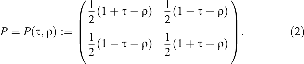
All entries of P must be nonnegative. This holds if and only if

We have equality in inequality (3) if and only if one of the entries of matrix (2) is 1, in which case we term P degenerate. For
Then,
Causes of Effects
While knowledge of the transition matrix P, and in particular the “average causal effect”
Using the notation
General causation:
That is, changing the value of X will result in a change to the value of Y. We can also describe this as “X affects Y.”
When the relevant variables (here X and Y) are clear from the context, we will simplify the notation to C.
Specific causation:
That is, changing the value of X from x to
We note that
Probability of Causation
In cases of interest, we will have observed

by consistency and no confounding.
Note that, unlike for the definition of the average causal effect, the probability of causation conditions on a value for the outcome. Our
Simple Bounds
The joint distribution for
Joint distribution of
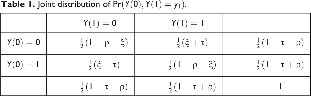
However, the internal entries of Table 1 are not determined by P but have one degree of freedom, expressed by the “slack” quantity

the probability of general causation.
The only constraints on

In particular
We further note


whence, by inequality (7),


Since
which is thus subject to the interval bounds, given by equation (10) or (11), as appropriate, divided by the known entry
This analysis delivers the following lower and upper bounds (superscript “s” for “simple”):


In the absence of additional information, the above bounds constitute the best available inference regarding the probability of causation.
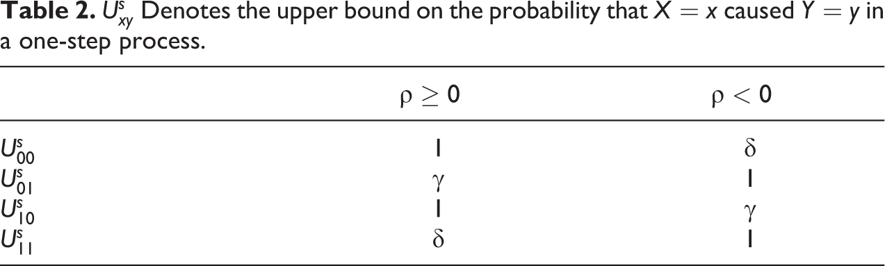
Specifically, when
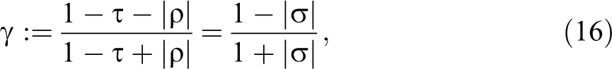
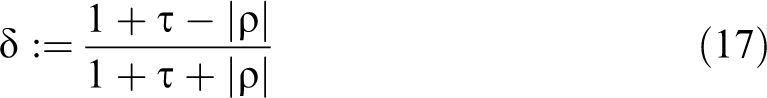
we have the upper bounds given in Table 2.
A particular interest is in cases where
and interval bounds given by

This result agrees with Tian and Pearl (2000) and Dawid (2011).
PC is identified (i.e., the interval inequality (19) reduces to a single point) if and only if
More generally, we have
Bounds From Mediation
We now suppose that, in addition to X and Y, we can gather data on one or more binary mediator variables
Assumptions
We confine attention to the case of a complete mediation sequence, where for every
where
We assume:
Consistency: Even when some or all of the previous M‘s are not set by intervention, the value of
No confounding: We have mutual independence between X,
Then,

Thus, the sequence
Finally, we assume that we have access to data sufficient to accurately determine the one-step transition probabilities

Inferences on Chains
In this section, we establish that the probability that X caused Y is given by the probabilities that each step in the chain from X to Y was caused by its predecessor.
Let the transition matrix from

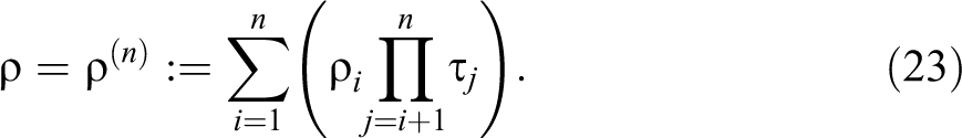
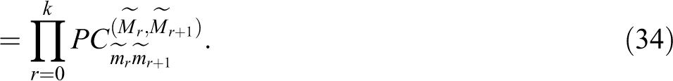
to indicate that we are assuming the above mediation sequence, and refer to equation (21) as a decomposition of the matrix P. In particular, we then have
We can readily show by induction that
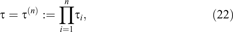
In particular, for the case

On account of equation (22), we have the following result:
Lemma 1: The average causal effect of X on Y is the product of the successive average causal effects of each variable in the sequence on the following one.
Lemma 2:
Proof
Suppose first that each variable affects the next. Then, changing the value of X will change that of M
1, which in turn will change that of M
2, and so on until the value of Y is changed, so showing that X affects Y. Conversely, if, for some
We have as a corollary that for any decomposition, the probability that X affects Y is the product of the probabilities that each variable in the sequence from X to Y affects the next in the sequence.
Corollary 1
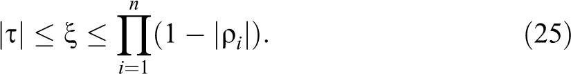
Given knowledge of the decomposition (21), the constraints on
Proof
By the assumed mutual independence of the
By equation (6).
On comparing inequality (25) with inequality (7), we see that detailed knowledge of the mediation process has not changed the lower bound for
Theorem 1
The upper bound that results from knowledge of the decomposition of P is no greater than the upper bound that results from P alone. It will be strictly less if for some
Proof
We compare the upper bound of inequality (25) with that of inequality (7).
Consider first the case


It follows that

Moreover, we shall have strict inequality in (27), and hence also in (28), if P
2 is nondegenerate and
Noting that if
We note that the above condition for strict inequality (28), while sufficient, is not necessary. For example, in the case
It follows from inequalities (25) and (28) that collapsing two mediators into a single one (for instance, by removing Mi
and replacing
Corollary 2
Consider two decompositions
Unobserved Mediators
Suppose first that, for the new case, we have observed
Indeed, in this case, equation (5) still applies, where
This analysis delivers the following revised bounds (superscript “
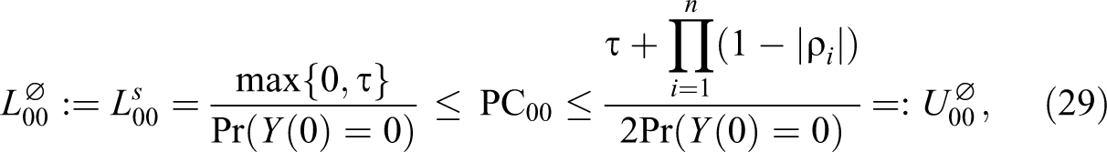
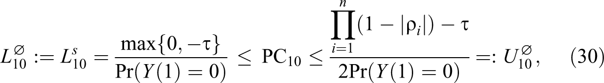
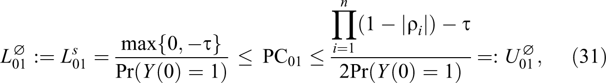
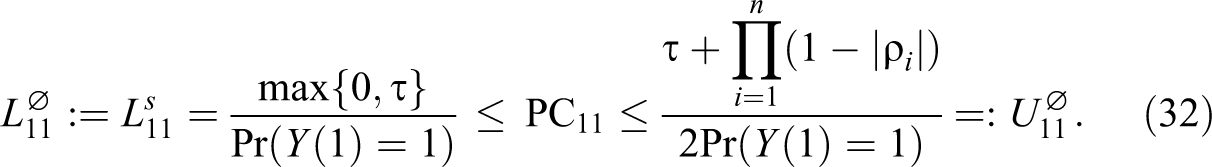
Note, in particular, for the case
For
Bounds When Some or All Mediators are Observed
Now suppose that, in addition to
The relevant probability of causation is now

Note that in contrast to the difference between equations (29)
–(32), on the one hand, and equations (12)
–(15), on the other hand, which relate to the same quantity
Theorem 2
Given observations on
Proof
From lemma 2, we have
whence, using the “no-confounding” independence properties,
□
Now since we have the decomposition information about the mediators (if any) occurring between
Again consider the special case with
It is easy to see that this lower bound can only increase if we introduce further observed mediators. It follows that the smallest lower bound occurs when there are no observed mediators, when it reduces to
In the remainder of this article, we shall give special attention to this case and write simply

The following result follows directly from the above considerations:
Lemma 3
The lower bound
However, it will follow from theorem 3 below that
Largest and Smallest Upper and Lower Bounds
Equation ( 34) provides a general formula for calculating bounds on the probability of causation for any pattern of data observed on mediating variables (including no data). We now use this result to assess the largest and smallest possible upper bounds from observation of possible values on mediating variables.
Consider an arbitrary decomposition of P:

with
We investigate the smallest and largest achievable values for
Theorem 3
Consider transition matrix
Largest and smallest achievable upper and lower bounds from decompositions of any length, given no mediators observed (
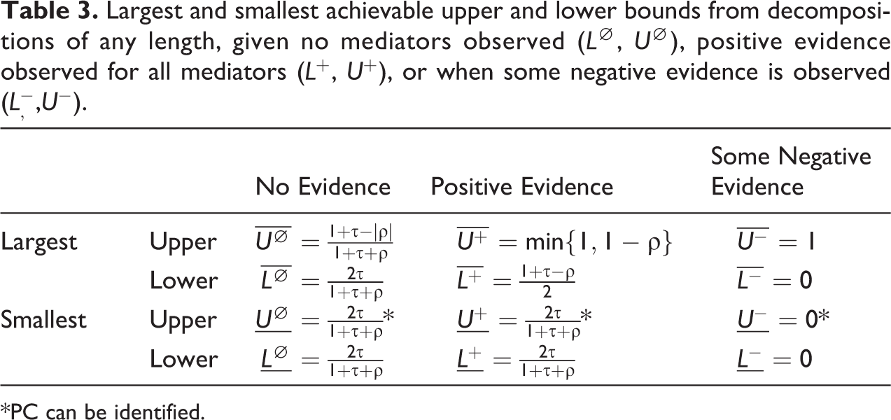
*PC can be identified.
Proof
See Online Appendix A (which can be found at Supplementary material for this article, available online).□
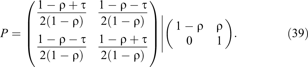
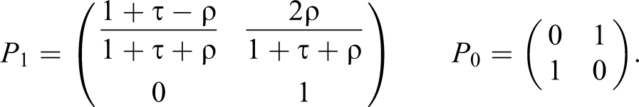
The largest upper bound with mediators unobserved,
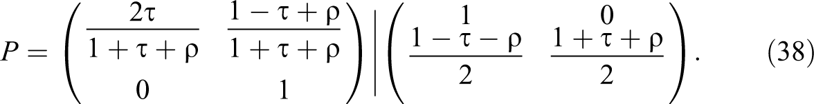
Note that, with this decomposition,
The smallest upper and lower bounds available when mediators are observed agree with the simple lower bound. Positive evidence cannot reduce the lower bound, but it can reduce the upper bound to the lower bound, at which point
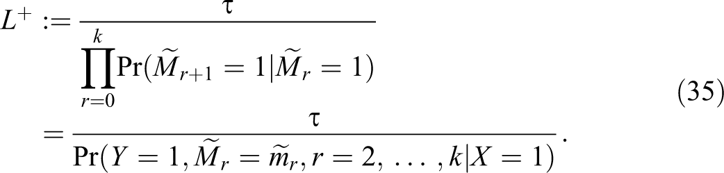
The largest upper bound with positive evidence on mediators,
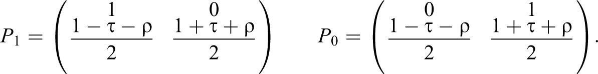
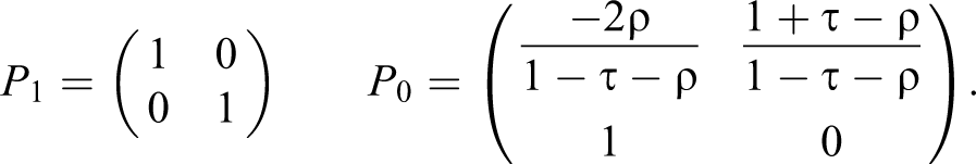
The lower bound can be raised with positive information on mediators and takes its largest value with the following degenerate two-term decomposition
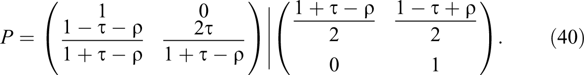
With this decomposition
For the case with some negative evidence on the mediators, the lower bound is always 0. The smallest upper bound is also 0, which can be achieved by the decomposition of equation (40) above, with the single mediator observed at 0 (the key feature of this decomposition is that

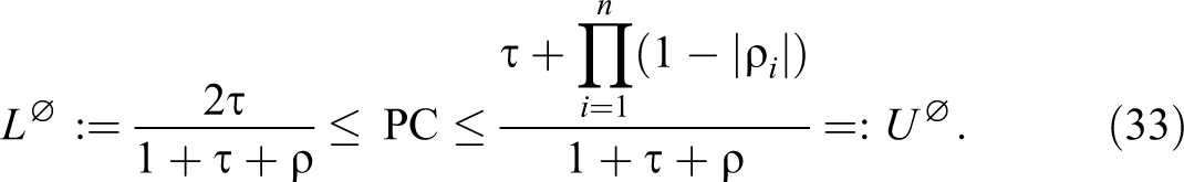
For

Comparisons
Although knowledge of mediators can narrow bounds, the scope for learning from knowledge of mediation processes—and the specific values taken on by mediators—is often small. In particular, although negative evidence can yield low upper bounds, providing confidence that an outcome was not due to a putative cause, positive evidence generally does not raise lower bounds substantially.
To put these claims in context, we compare the extrema on bounds in theorem 3 with bounds that can be achieved from “homogeneous” processes, from knowledge of monotonicity, and from covariate information.
Homogeneous Processes
First, we consider bounds for a special case: long homogeneous processes—that is, cases in which we have a potentially unlimited sequence of variables directly mediating between X and Y, with one-step transition matrices that are identical at each step (and having positive average causal effect). For such processes,
Intuitively, a lot of data at many points in a chain should lead to stronger inferences. This intuition is however not in line with our finding that the extrema on the bounds given in theorem 3 are generally achieved through two-step processes in which transition matrix P 1 is different from transition matrix P 2. The bounds from long processes can be no better than those described in theorem 3, but how different are they?
Table 4 shows the upper and lower bounds achievable with homogeneous processes of unbounded length, for three cases: cases in which there are no data on the values of the mediators, cases in which all mediators are observed and positive (Mt = 1 for all t), and cases in which values alternate between 1 and 0. For further details, see Online Appendix B (which can be found at Supplementary material for this article is available online).
Upper and lower bounds from homogeneous decompositions of length
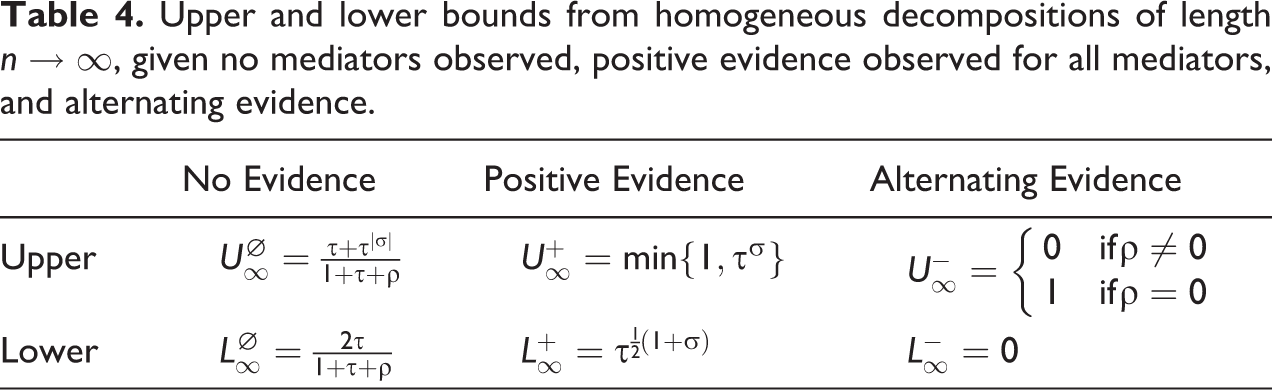
We see that, for
Monotonicity
Suppose that we knew that there are no cases for which the exposure would prevent the outcome, that is, such that
From Table 1, we have that monotonicity implies
Observed Covariate
Suppose that, in addition to X and Y, we can observe a binary covariate W, pretreatment to X, which can affect the dependence of Y on X. Let
In particular, it could then be the case that
In this case, knowledge that an individual with
Unobserved Covariate
As shown in Dawid (2011), knowledge of covariates can improve bounds, even if their values are not observed for the case at hand. In particular, this can let us identify PC at the upper bound, For
For
In either case, knowledge that
Figure 1 compares the bounds obtained, under various assumptions, for a range of values of
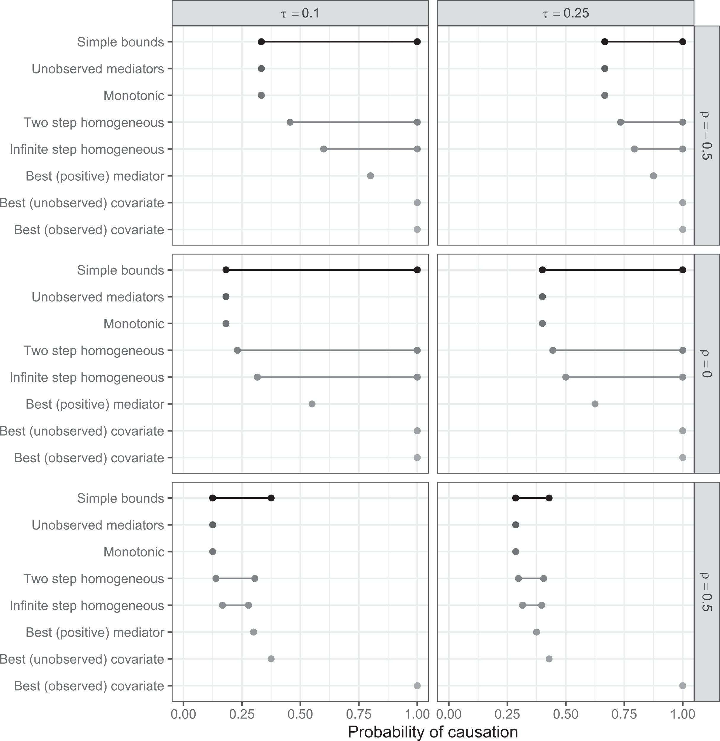
Comparison of bounds on PC. Simple bounds are derived from the distribution of Y given X and are given by inequality (19). Tightest bounds from unobserved mediators are given by the decomposition in (38). Monotonicity implies the same bounds. Bounds from a homogeneous two-step decomposition and positive evidence can be calculated from theorem 3. Infinite-step bounds, assuming positive evidence observed at every step from a homogeneous process, are given in Table 4. Best two-step bounds show the highest lower bound achievable from information on mediation shown in Table 3 and can be achieved with positive evidence for the decomposition of equation (40). Greatest lower bounds given information on an unobserved and observed binary covariate are as described in the Comparisons section.
Conclusion
We provide a general formula for calculating bounds on the probability of causation for complete mediation processes involving binary variables of arbitrary length and with arbitrary data patterns. In addition, we characterize the largest and smallest achievable bounds obtainable from any data. Knowledge of these bounds is useful for assessing when there can be gains from learning about processes in a population and gains from learning about the values of mediators for cases.
Our analysis focuses on ideal cases in which there is a very simple known causal structure in which nodes are connected in a simple causal chain—excluding situations such as one in which X has a direct effect on Y as well as an indirect effect through M. We show, however, that even in these ideal conditions, access to even unlimited data on mediators has only a modest, and asymmetric, impact on inferences. Knowledge of mediation processes, and of positive values for some mediators in a particular case, can raise the lower bound on the probability of causation, thus providing some evidence against a skeptic who doubts that the outcome in the case can be attributed to the putative cause. Moreover, this information can be enough to achieve identification. However, the gains are generally modest and may not be sufficient to convince a skeptic. For instance, if most outcomes are positive for untreated units, then it follows from our results that there is no evidence on mediators for a treated unit with positive outcomes that can raise the lower bound on the probability that the outcome was due to the treatment above 50 percent. More generally, identification at 1 is not possible. In contrast, for some processes, observing negative evidence on a single mediator can effectively convince a skeptic that the outcome is not due to the exposure.
These general results have implications for when gathering further intermediate data on particular cases can be useful. We see, for instance, starkly contrasting implications for a process in which X is a necessary condition for a sufficient condition for Y and a process in which X is a sufficient condition for a necessary condition for Y. In the first case, consistent with arguments in Mahoney (2012), negative evidence on mediators implies no causal effect—we have a hoop test. In addition, we show, positive evidence on mediators yields the largest possible upper bound and identifies the probability of causation. For example, if it is known that the effect of delivering a deworming medicine passes uniquely through ingestion, and ingestion is sufficient for effective deworming, then evidence of ingestion raises the lower bound and identifies the probability of causation. These features, we note, depend on the chain structure we specify: were there a possible direct effect from X to Y, then necessity followed by sufficiency would not imply a hoop test because knowledge that X did not cause M is not sufficient to conclude that X did not cause Y.
In contrast for a process in which X is a sufficient condition for a necessary condition for Y, we already enjoy identification and there is no gain from gathering data on the mediator. For instance, if ingesting medicine is a sufficient condition for good health, and good health is a necessary condition for good school performance, then observing ingestion and good school performance is sufficient to achieve identification. There are no additional gains from measuring health, since good health is already implied by good performance. A similar logic holds for any chain of necessary relations, suggesting that these do not in fact aggregate to form a smoking gun test since if
The main result can also be used to guide choice of which causal process observations to examine. For instance, consider a homogeneous process with n steps (n even) and suppose that researchers can observe the value of just one mediator Mi . In this case, we can show that the lower bound on the probability of causation, following observation of positive data, is maximized if the central mediator in the sequence is observed. For intuition, there is more ex ante certainty about the values of mediators close to the edges; ex ante uncertainty increases, and the scope for learning increases accordingly far from the edges. See Appendix C for details.
Finally, these results also have implications for the potential gains from research agendas that seek to learn about mediation processes (as, e.g., in the designs described in Imai, Keele, and Tingley 2010) compared to the potential gains from learning about effect heterogeneity (as, e.g., is done in factorial designs; Fisher 1926). The scope for gains from knowledge of mediation processes is typically weaker than potential gains from knowledge of conditions under which interventions are more or less effective. While of course the actual gains from knowledge of mediators and covariates depends on underlying causal relations, by providing extrema on bounds, the results we provide can inform the choice of experimental design.
Supplemental Material
Supplemental Material, sj-pdf-1-smr-10.1177_00491241211036161 - Bounding Causes of Effects With Mediators
Supplemental Material, sj-pdf-1-smr-10.1177_00491241211036161 for Bounding Causes of Effects With Mediators by Philip Dawid, Macartan Humphreys and Monica Musio in Sociological Methods & Research
Footnotes
Authors’ Note
Monica Musio’s research supported by the project GESTA of the Fondazione di Sardegna and Regione Autonoma di Sardegna, Sardegna, Italy.
Acknowledgment
The authors thank Steffen Huck, Alan Jacobs, Lily Medina, and Michael Zürn for their generous comments.
Declaration of Conflicting Interests
The author(s) declared no potential conflicts of interest with respect to the research, authorship, and/or publication of this article.
Funding
The author(s) received no financial support for the research, authorship, and/or publication of this article.
Supplemental Material
The supplemental material is available in the online version of the article.
Notes
References
Supplementary Material
Please find the following supplemental material available below.
For Open Access articles published under a Creative Commons License, all supplemental material carries the same license as the article it is associated with.
For non-Open Access articles published, all supplemental material carries a non-exclusive license, and permission requests for re-use of supplemental material or any part of supplemental material shall be sent directly to the copyright owner as specified in the copyright notice associated with the article.