
Abstract
This study reviews and compares indicators that can serve to characterize numerically the nature of state sequences. It also introduces several new indicators. Alongside basic measures such as the length, the number of visited distinct states, and the number of state changes, we shall consider composite measures such as turbulence and the complexity index, and measures that take account of the nature (e.g., positive vs. negative or ranking) of the states. The discussion points out the strange behavior of some of the measures—Elzinga’s turbulence and the precarity index of Ritschard, Bussi, and O’Reilly in particular—and propositions are made to avoid these flaws. The usage of the indicators is illustrated with two applications using data from the Swiss Household Panel. The first application tests the U-shape hypothesis about the evolution of life satisfaction along the life course, and the second one examines the scarring effect of earlier employment sequences.
Keywords
When considering individual state sequences describing, for instance, time use, spatial development, course of health and well-being, or life trajectories such as occupational careers and cohabitation pathways, it is of interest to quantitatively describe the nature of the sequences. For example, we may want to distinguish smooth careers from more chaotic ones, stable from unpredictable family trajectories, and improving from deteriorating health pathways. Quantitative characteristics that can easily be summarized with means and standard deviations, for example, are also useful for synthetically describing sets of sequences.
Summary indicators of individual sequences have been used in many different studies. To mention just a few, Brzinsky-Fay (2007) uses individual indicators to study school-to-work transitions, Biemann et al. (2011) investigate career complexity over time, Manzoni and Mooi-Reci (2018) examine the quality of professional careers after an initial spell of unemployment, Christensen (2021) compares the stability of the careers among different groups of elite tax professionals, Elzinga and Liefbroer (2007) study the destandardization of family-life trajectories across different countries, Widmer and Ritschard (2009) study the destandardization of cohabitational and occupational trajectories across birth cohorts, Van Winkle (2020) studies family-life course complexity across twentieth-century Europe, Hiekel and Vidal (2020) study the complexity in partnership life courses, and Mattioli, Anable, and Vrotsou (2016) study the occurrences of activities linked with car use in time-use sequences.
Here, we review the individual sequence indicators used in these works and make some new propositions. We compare the indicators and stress what aspect of the nature of the sequence they attempt to catch.
In sequence analysis, the conventional approach to characterize individual sequences employs comparison with the other sequences in the data set. Typically, pairwise dissimilarities between sequences are first computed. These dissimilarities are then used to cluster the sequences; this allows to characterize each individual sequence by the group to which it belongs. In contrast, this study focuses on intrinsic individual characteristics of the sequences, that is, characteristics that can be computed regardless of the other sequences.
Table 1 lists the indicators addressed. Sequences are typically represented as a succession of states, for example, FFPPPU. It is also common to represent sequences as a succession of spells in different states. For example, FFPPPU can equivalently be represented as F/2-P/3-U/1 where F/2 indicates a spell of length 2 in F. The table indicates for each indicator whether it focuses on the characteristics of state representation or spell representation.
Individual Characteristics of Sequences.
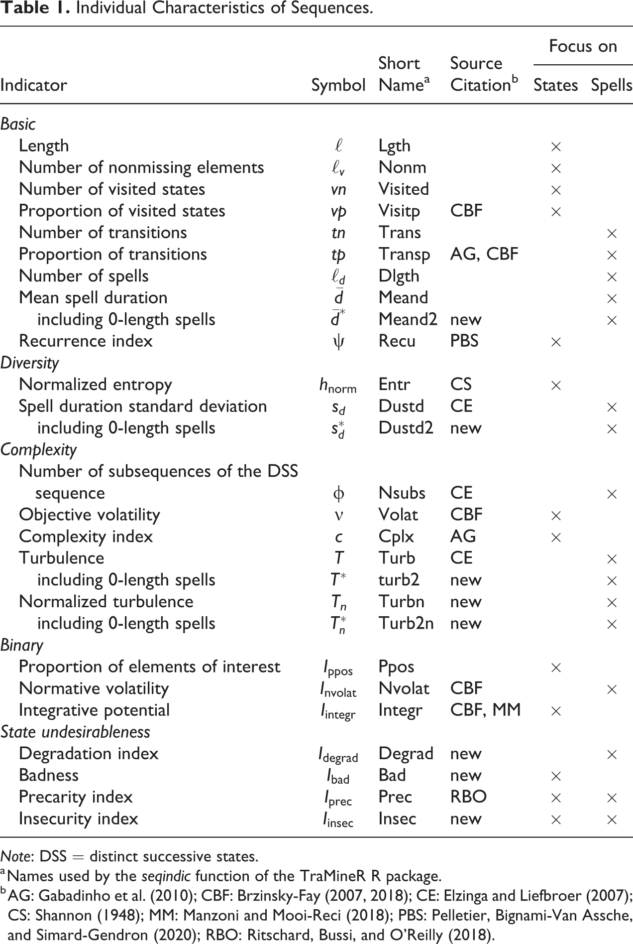
Note: DSS = distinct successive states.
a Names used by the seqindic function of the TraMineR R package.
We distinguish four types of measures: basic sequence characteristics, measures of diversity within the sequence, measures of complexity of the sequence, and measures of (un)favorableness of the sequence.
Basic measures are essentially simple counts such as sequence length, number of visited states, and number of state changes. Within-sequence diversity concerns the diversity of not only the states but also spell durations. Complexity refers primarily to the arrangement of the states within the sequence.
State sequences are successions of elements taken from a finite alphabet A (set of possible states). The first three types of measures apply irrespective of the states. For example, the value of the measures will be the same for the sequences FFFUU and PPPFF where F stands for full-time work, P for part-time work, and U for unemployment. The last group of measures (unfavorableness), on contrary, requires additional information on the nature of the states either as a distinction between positive and negative states, for example, {F, P} versus U, or as a preference order among the states such as
The scope of the measures is demonstrated through two applications to data from the Swiss Household Panel (SHP). The first application compares the life satisfaction over 19 years reported annually by younger, middle-aged, and elder adults and shows how the indicators can serve to study the U-shape issue of the evolution of satisfaction along the life course (Bartram 2021; Blanchflower and Oswald 2008; Frijters and Beatton 2012). The second application uses monthly work statuses to illustrate how individual indicators can serve to study the scarring effect of earlier employment trajectories (Abebe et al. 2016; Manzoni and Mooi-Reci 2011).
Alongside the description of indicators, the discussion provides, when necessary, indications of interest for the interpretation of measures such as the range of possible values and characterization of configurations corresponding to the minimum and maximum values. In addition, a small set of 16 toy sequences is used to illustrate how the measures rank the sequences. These examples permit to highlight unexpected behaviors of, in particular, the turbulence of Elzinga and Liefbroer (2007) and the precarity index of Ritschard et al. (2018). Alternatives are proposed to avoid these unwanted behaviors. The newly proposed measures include the mean and standard deviation of spell durations that take account of nonvisited states, revised turbulence, degradation index, badness index, and insecurity index, the latter being a revised precarity index.
All addressed indicators including the newly proposed ones have been implemented in the latest release (version 2.2-2) of the TraMineR R package (Gabadinho et al. 2011) and can be obtained with the seqindic function. The short names shown in Table 1 are those used by seqindic.
Individual Sequence Measures
The section successively reviews indicators of basic features, within-sequence diversity, complexity, and (un)favorableness. For the latter group, we distinguish between measures based on a dichotomization of the state space and a preference order of the states or possibly on the undesirableness degrees of the states.
To illustrate the addressed measures, we consider the 16 sequences of length 8 displayed in the first column of Table 2. The alphabet comprises four work statuses: F, full-time work; P, part-time work; T, training; and U, unemployment. The sequences are roughly sorted from the most complicated to the simplest ones. For measures based on a dichotomization, we oppose the positive states F and P to the others, and for indicators based on a preference order, we assume
Example Sequences: Diversity Indicators.
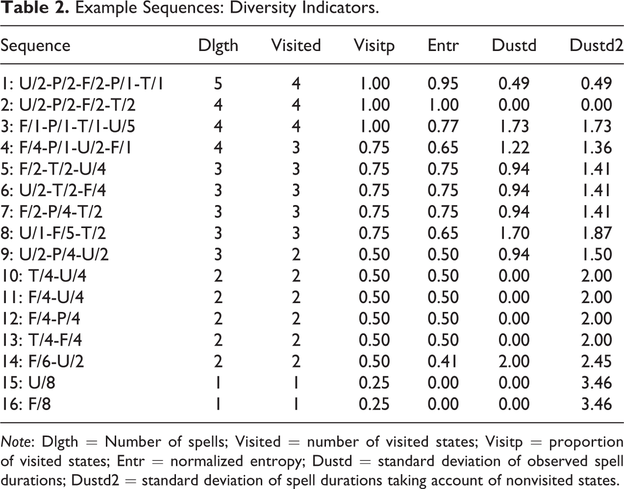
Note: Dlgth = Number of spells; Visited = number of visited states; Visitp = proportion of visited states; Entr = normalized entropy; Dustd = standard deviation of observed spell durations; Dustd2 = standard deviation of spell durations taking account of nonvisited states.
Basic Features
Basic characteristics of a sequence include the length
When the interest is in spells (in a same state) rather than states, we may consider the sequence of distinct successive states (DSS) where we ignore the successive repetition of states. For example, the DSS of the sequence FFUUUP is FUP. The length
The average number of visits to visited states proposed by Pelletier et al. (2020) that we denote here
Within-Sequence Diversity
The diversity within a sequence refers to either the diversity of states visited or the diversity of spell durations. The number
Longitudinal entropy
The entropy considered here is a statistical measure borrowed from information science (Shannon 1948) where it serves to measure the average amount of bits necessary to unambiguously encode a message. In statistics, entropy reflects the level of uncertainty or unpredictability of an outcome. The higher the diversity of possible outcomes, the higher is the uncertainty. Typically, entropy is applied to a discrete distribution. In our case, it is the state distribution within the sequence, and the entropy measures the diversity of states in the sequence. The state distribution can also be seen as the time distribution among the different states. Let
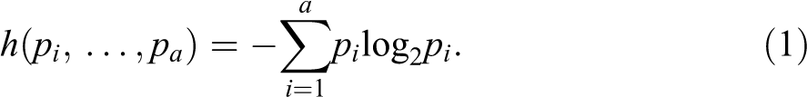
The diversity (uncertainty) is null and the entropy is zero when a same state, say j, is observed all along the sequence in which case
Shannon’s entropy is the most commonly used diversity measure for categorical outcomes. However, there exist other diversity measures such as the Gini–Simpson index
In Table 2, we can observe how the entropy nuances the proportion of visited states. Sequences 11 and 14, for example, have the same proportion
Variance of spell length
While entropy and proportion of visited states measure the diversity of the states, this third measure focuses on spell durations. Elzinga and Liefbroer (2007) use the inverse of this variance in the definition of their turbulence index (see Complexity of the State Arrangement subsection) as a measure of the unpredictability of spell duration. However, the variance considered by these authors, that is,
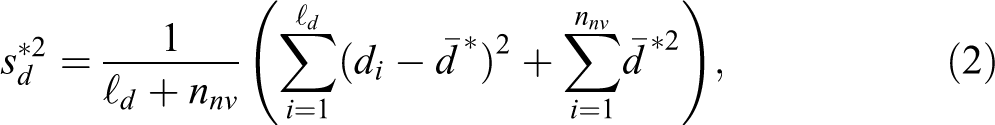
where di
is the duration of the ith spell,
The variance
Since this is a variance, it may be more suitable for interpretation purposes to look at its square root, that is, at the standard deviation. These are the values reported in Table 2. The standard deviations Dustd (sd
) that does not take account of nonvisited states and Dustd2 (
Complexity of the State Arrangement
Complexity of the sequence refers to the instability or unpredictability of state arrangement in the sequence. It involves multiple aspects, and complexity increases with, for example, the number of state changes, number of visited states, and unpredictability of the time spent in the states or of the spell durations.
The number of spells
Another rough characteristic of interest suggested by Elzinga (2010) (see also Elzinga and Liefbroer 2007) is the number of distinct subsequences that can be extracted from the sequence. For example, sequence FFU contains six subsequences {}, F, U, FF, FU, FFU while the more simple sequence FFF contains only four subsequences{}, F, FF, FFF. Elzinga considers the number
Example Sequences: Complexity Indicators.
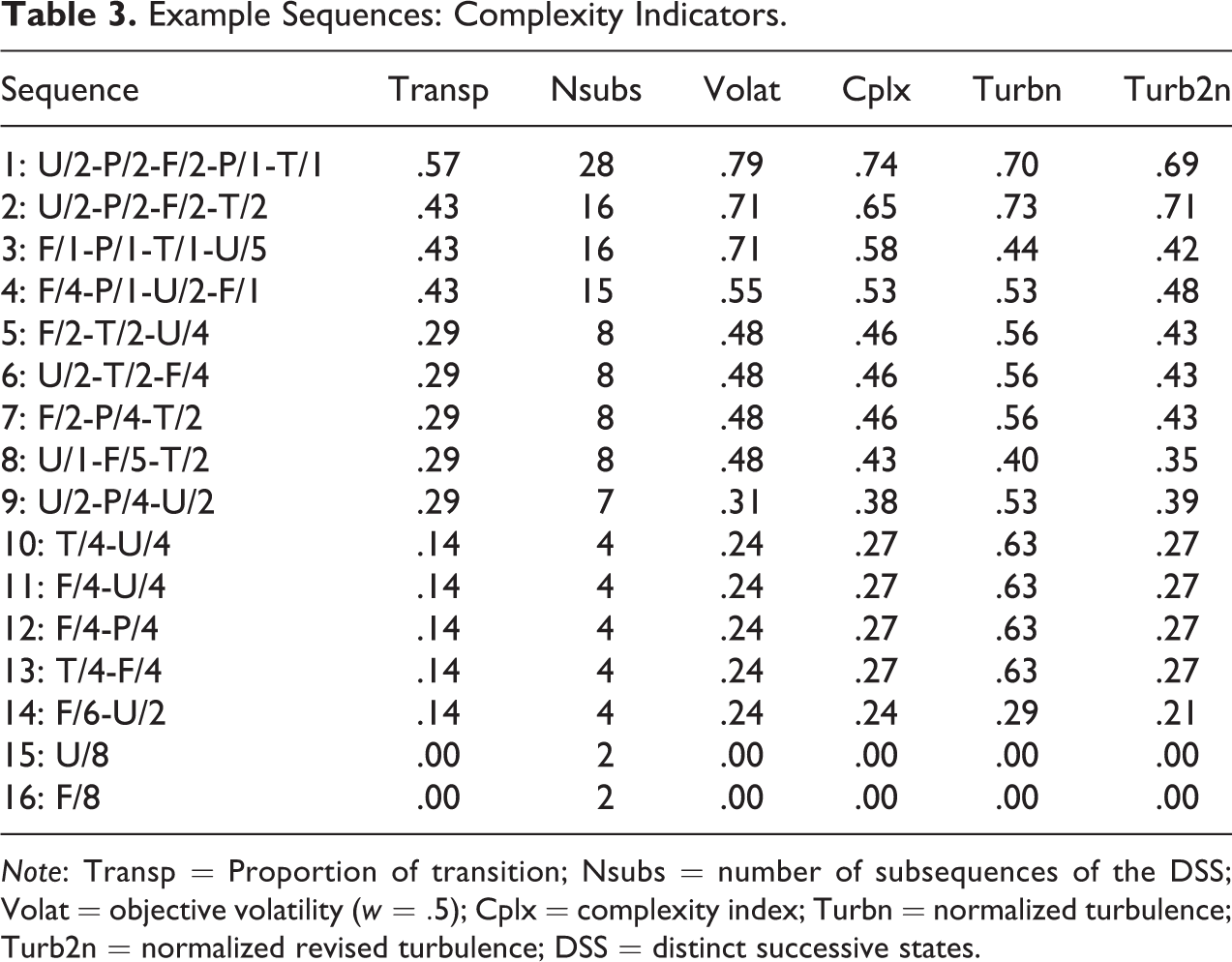
Note: Transp = Proportion of transition; Nsubs = number of subsequences of the DSS; Volat = objective volatility (
At least three refined measures of complexity attempt to capture simultaneously several aspects by combining one of the above rough measures of arrangement with a measure of within-sequence diversity.
Objective volatility
Brzinsky-Fay (2018) distinguishes normative volatility (first introduced in Brzinsky-Fay 2007) and objective volatility. Normative volatility requires to distinguish between positive and negative states and will, therefore, be addressed in Taking the Nature of the States Into Account subsection.
The objective volatility

with
From the complexity point of view,
Complexity index
The complexity index of Gabadinho et al. (2010, 2011) adjusts the proportion of transitions to take account of the diversity of visited states, the latter reflecting the unpredictability of elements in the sequence. Formally, the index is defined as the geometric mean between the proportion

The complexity is normalized by construction,
Turbulence
Turbulence (Elzinga and Liefbroer 2007) is based on the number
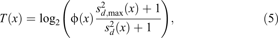
where
We have
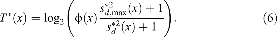
Now that we have the maximum value, to get an index within the
Table 3 reports these normalized turbulence values for our example together with the other complexity indexes. We see that all measures are positively correlated. We also observe that the complexity index and turbulence exhibit more different values than volatility and Elzinga’s
It is instructive to look at Figure 1 that displays the sequences sorted in decreasing order according to the complexity, turbulence, and revised turbulence indexes, respectively. On the one hand, the order defined by the original turbulence strongly differs from the other two. In particular, we observe the strange behavior of the turbulence that ranks the quite simple sequences 10–13 among the most turbulent sequences. On the other hand, the plot confirms that the revised turbulence and complexity index behave similarly. The most noticeable difference is sequence 3 that gets a lower revised turbulence value despite its three transitions than sequences 5–7 that have only two transitions. This is due to the relatively high duration variance in sequence 3 (see Dustd2 in Table 2).
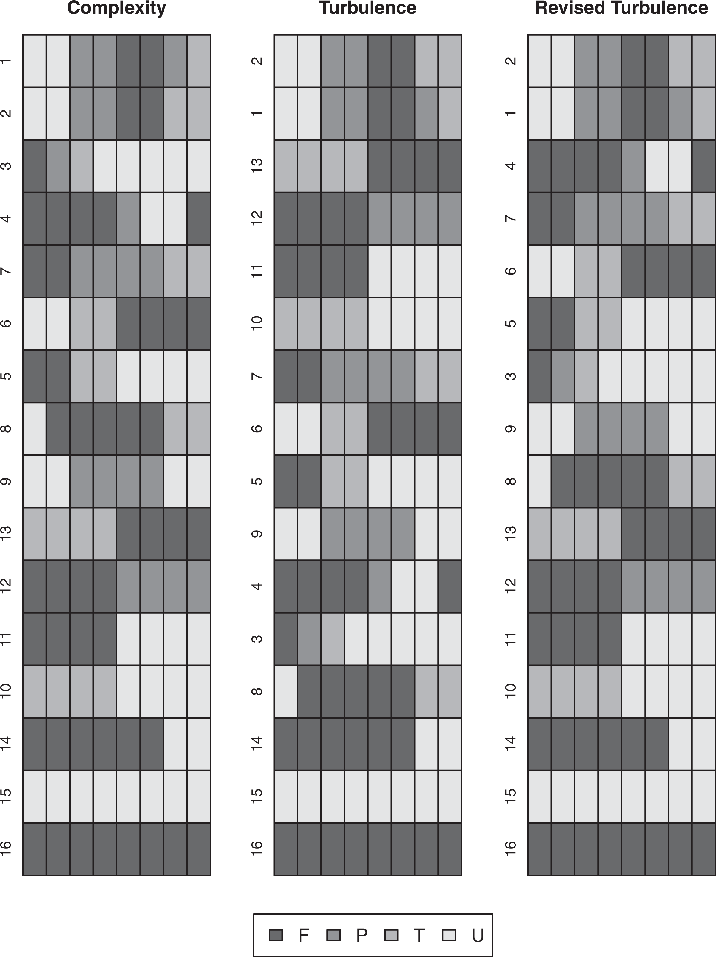
Sequences sorted by decreasing order of complexity measures.
Taking the Nature of the States Into Account
In some situations, we can qualify states in the alphabet as good or bad, positive or negative, desired or unwanted, or success or failure. Typically, “employed” is positively qualified and “unemployed” is considered as a negative state. More generally, we may want to oppose states of interest to the other states. In other cases, we may have an order of preference or at least a partial order of preference of states, for example, full-time work preferred to part-time work, which in turn is preferred to unemployment. The latter example would be a partial order if an additional state that we do not know how to rank—inactivity, for example—would come into play or if some states would be considered as equivalent. The measures considered so far ignore such information. However, there exists a series of indexes specifically designed to take account of a binary distinction between states, a preference order of the states, or even levels of undesirableness of the states. We start with measures based on a binary distinction between states.
Distinguishing positive and negative states
When some states can be qualified as positive, we can associate a binary sequence of positive (good, of interest) and nonpositive (bad, not of interest) states to each sequence. In particular when the focus is on a specific state of interest such as having a job or having a child, for example, we can qualify this state as positive and oppose it to all other states. From such binary sequences, we can derive the following indicators:
The proportion of positive elements
The integrative potential or capability is another indicator introduced by Brzinsky-Fay (2007). It measures the tendency to integrate a positive state (employment in Brzinsky-Fay 2007), that is, reach a positive state and then stay in a positive state. Formally, letting
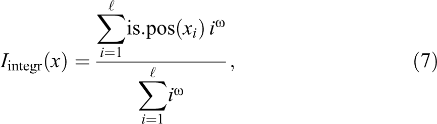
where
By construction, the proportion of positive elements, normative volatility, and integrative potential
By dichotomizing one state s against all other states, we can compute the integrative potential for any state s. We shall denote this index as
Table 4 exhibits the values of the potential
Indicators Based on State Dichotomization, Positive States {F, P}.
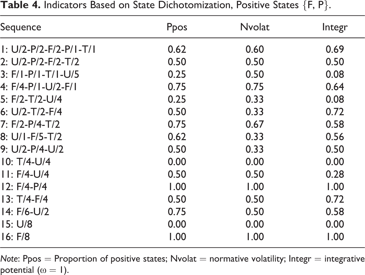
Note: Ppos = Proportion of positive states; Nvolat = normative volatility; Integr = integrative potential (
State undesirableness levels
Instead of a simple dichotomization between positive and other states, we may dispose of finer information about the (un)desirableness level of the states. The simplest such information would be a preference order among the elements of the alphabet or at least a partial preference order, that is, an order on a subset only of the states. The first ranked state would be the preferred state, and the last one would be the most undesirable. The rank can serve as undesirableness degree of the states. Sometimes, however, we may dispose of richer information on the undesirableness of the states. For example, the values reported in Table 5 were obtained by specifying the undesirableness degrees
Indicators Based on State Undesirableness
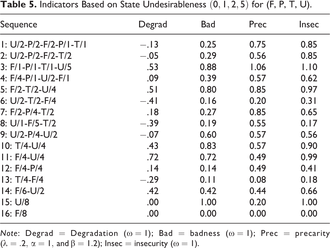
Note: Degrad = Degradation (
First, considering only the preference order, we can count the number of upward and downward state changes and compute the proportions

In case of a partial state order, transitions to and from noncomparable states—states that cannot be ranked—and transitions between states belonging to a same equivalence class will be ignored.
By construction,
The index can be tuned by using transition weights in the calculation of the downward and upward proportions
Here, in addition, we suggest to weight each transition by the potential to integrate the spell that follows the transition. The potential
A second index, badness, attempts to measure the overall badness degree of the sequence. We define it as the sum of the undesirableness degrees of the visited states each weighted by the potential to integrate the state. This way, the weight of each state increases with the number of occurrences and recency, that is, states occurring near the end of the sequence contribute more to the overall badness degree of the sequence. Formally, letting

We have
The precarity index proposed by Ritschard et al. (2018) is based on the idea that precarity has to do with the instability of the sequence and that this instability can be measured by the complexity index. Complexity in itself is a rough precarity indicator that should be amplified when complexity results from deteriorating events (downward transitions) and reduced in case of improving events (upward transitions). This amplification/reduction mechanism is operationalized multiplicatively, that is, by multiplying the complexity index by a correction factor that should be greater than 1 when there is a majority of downward transitions and lesser than 1 in case of a majority of upward transitions. In addition, the index takes account of the undesirableness of the start state so that, among two sequences with similar corrected complexity, the sequence with the less favorable start state gets the higher precarity value.
Typically, the multiplicative correction factor of the complexity is defined as

where
The (too) many tuning possibilities may hamper the usage of the precarity index. In addition, by mixing additively the undesirableness of the start state and corrected complexity, that is, two quantities that are not measured on the same scale, the index becomes very hard to interpret. It also has some strange behavior. With a low
We propose insecurity as an alternative and simpler index. We postulate that insecurity results from instability, tendency to degradation, and high undesirableness. As for the precarity, we use complexity as an indicator of instability and adjust it with the degradation index to distinguish complexity resulting from improving changes from complexity resulting from degradation. In addition, we need a level component to distinguish between complexity occurring among undesirable states and complexity among more favorable states. We fix this level by means of the undesirableness of the first spell. Unlike the multiplicative form in the definition of

In the first term—undesirableness of the first spell—the undesirableness
For sequence 14 and
Simply summing the complexity index, degradation index (that takes negative values in case of improving changes), and undesirableness of the first spell facilitates the interpretation of the index because differences in insecurity values can then be straightforwardly expressed in terms of any of the three components. Looking for example at sequences 7 and 8, the difference in insecurity is
For sequences made of a single spell such as sequences 15 and 16, the complexity and degradation indexes are 0, and the potential to integrate the first spell is 1. In such cases, the insecurity
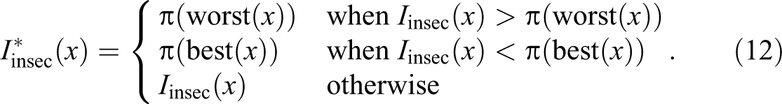
For example, sequence 7, whose worst state is T, gets an insecurity value
While the bounded insecurity
Looking at Figure 2 that displays the sequences sorted according to the degradation, badness, and insecurity indexes, we see that the three indexes behave quite differently. As expected, badness essentially summarizes the undesirableness of the elements of the sequence and the degradation index summarizes the tendency to deterioration. The behavior of the insecurity index resembles more badness than degradation. The most noticeable differences between badness and insecurity concern the most complex sequences 1 and 2 that appear among the upper half of the most insecure sequences and in the lower half regarding badness. Although the three indexes behave differently, they are generally positively correlated as can be seen in Figures 4 and 5 based on values from the two applications below. Another point worth mentioning is that sequences with a similar structure such as sequences 5–7 or 10–13 get the same values for all indicators in Tables 2 and 3 while they get different values once we take account of the nature of the states in Tables 4 and 5.
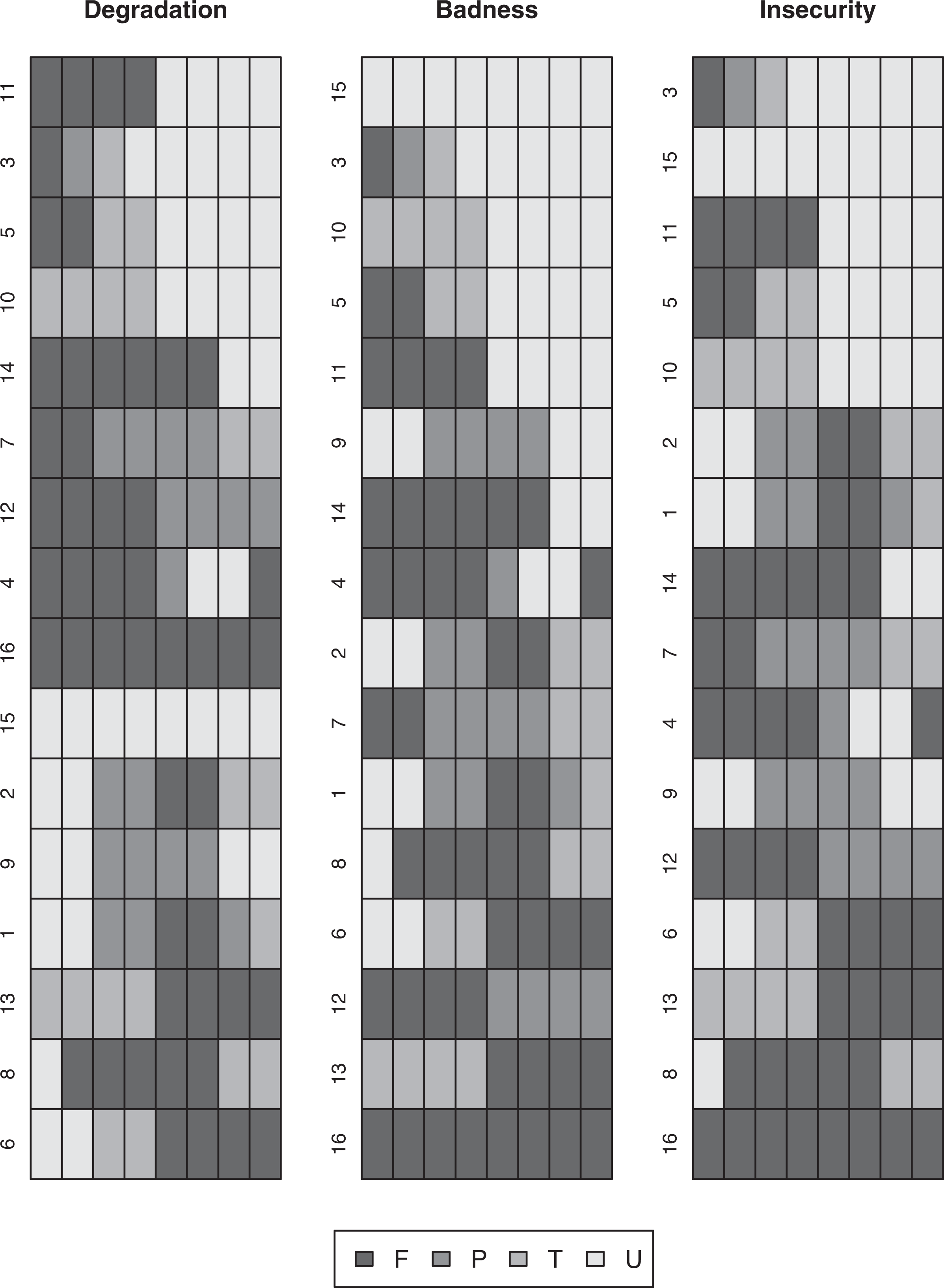
Sequences sorted by decreasing order of unfavorableness indicators.
Life Satisfaction in Switzerland
As a first application, we show how individual indicators could be invoked to address the controversial issue of whether the evolution of life satisfaction along the life is U-shaped or not (Bartram 2021; Blanchflower and Oswald 2008; Frijters and Beatton 2012). We consider for that the variable “Satisfaction in general with Life” from the SHP. This is a scale variable with 11 possible values ranging from 0 to 10, 0 meaning “not at all satisfied” and 10 “completely satisfied.” Data on this variable are available since wave 2 (2000), and we use data up to wave 20 (2018). However, because of attrition and the introduction of additional samples in 2004 and 2013, the data for most of the individuals cover only shorter periods. Here, we retain 19-year-long life satisfaction sequences with at least 10 valid values among the 19. This leaves us with 6,002 individuals, of which 864 are youngsters (born after 1980), 2,072 are middle-aged people (born between 1961 and 1980), and 3,066 are elder people (born in 1960 or earlier). The sequences were aligned on the first valid state and then truncated at length 15 to drastically reduce the number of ending missing elements.
The index plots in Figure 3 show that the sequences look quite complex with many transitions for all three groups. There is no clear difference between the groups, except the slightly higher proportion of youngsters who start their observed satisfaction trajectory in one of the top two response categories (dark blue). The plots do not exhibit any obvious improving or deteriorating tendency for any group.
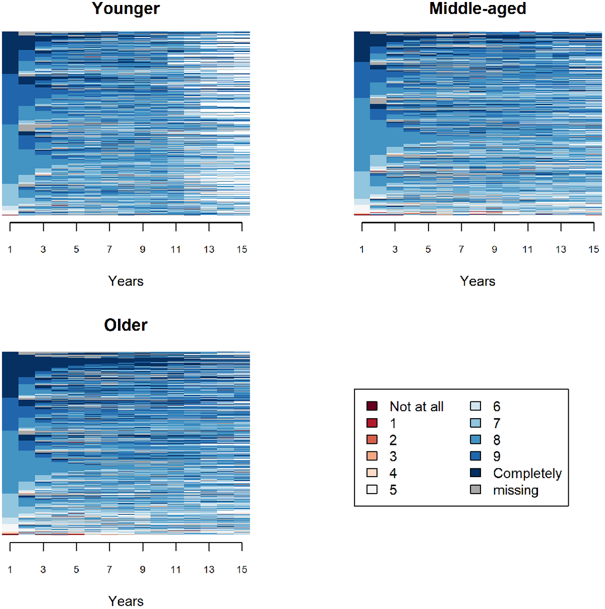
Index plots of life satisfaction by birth cohort.
Table 6 reports mean values of a selection of indicators. The first five—that is, Visitp, Transp, Entr, Cplx, and Turb2n—have been retained only for illustration while the last four serve for commenting the U-shape hypothesis. The integrative potential (Integr) was computed by considering the top two categories as positive and measures based on the state order (Bad, Degrad, and Insec) by assuming equidistant undesirableness degrees for the 11 life satisfaction values. The recency exponent was set as
Mean Values of Indicators for Life Satisfaction Trajectories and Student t of Pairwise Differences.
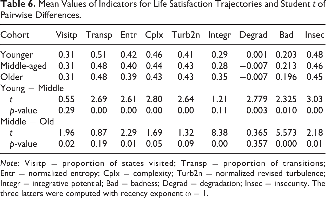
Note: Visitp = proportion of states visited; Transp = proportion of transitions; Entr = normalized entropy; Cplx = complexity; Turb2n = normalized revised turbulence; Integr = integrative potential; Bad = badness; Degrad = degradation; Insec = insecurity. The three latters were computed with recency exponent
Since some sequences are shorter than others, it is worth mentioning that because the indexes are all either proportions or derived from proportions, none of them depends on the sequence length. It is, thus, legitimate to average and compare index values of sequences of different lengths. Regarding the gaps remaining in the sequences, there are two options: either treat the gap as a noncomparable element of the alphabet or simply ignore it. Here, we retained the latter option. However, the results are almost identical to those of the first option. We also obtain very similar results when deleting all sequences containing gaps.
As we could expect from the index plots, the reported mean values do not reveal drastic differences between groups. Nevertheless, at least one difference between age groups is statistically significant for each indicator. Thus, the individual indicators prove useful to point out relevant nonobvious differences.
Interestingly, when looking at the complexity and revised turbulence indexes, we see that while trajectories of youngsters tend to be slightly more complex than those of the other two groups, trajectories of middle-aged and elder persons tend to be more turbulent. This seemingly contradicting outcome is possibly due to the different ways complexity and turbulence take time into account. The turbulence index depends on the distribution of spell durations while the complexity index depends on the distribution of total time spent in each of the states. These may be quite different when there are multiple spells in the same state, as is the case here with an average recurrence index of 2.3 for youngsters and 2.5 for middle-aged and elder people.
Ideally, to test the U-shape hypothesis, we should be able to follow up with people along the whole life course. However, we follow individuals over periods of 15 years only with our data. In compensation, we have data for three age groups. From the U-shape hypothesis, we expect the following:
The results in Table 6 confirm such tendencies with some nuances. Although the degradation index suggests more a reversed-L-shape (flat for youngsters and improving for the other two groups) than a U-shape, there is no evidence against Hypothesis 1. The mean badness values behave as expected across age groups. Since the differences are statistically significant, this provides evidence in favor of Hypothesis 2. The values for integrating favorable states confirm Hypothesis 3 only partially. Like the degradation index, they suggest a reversed-L-shape but with improvement only for the older group. Finally, the insecurity values support Hypothesis 4 with statistically significant decreases between youngsters and middle-aged people and between middle-aged and elder people.
In conclusion, the average values of the indicators provide some evidence of increasing average satisfaction for aged people but no clear evidence of decreasing satisfaction during early life. As such, they do not contradict the U-shape hypothesis. However, if this is true as a tendency at the aggregate level, there is relatively high variability among individuals as can be seen in Figure 4. In particular, most of the degradation values of elder people range between
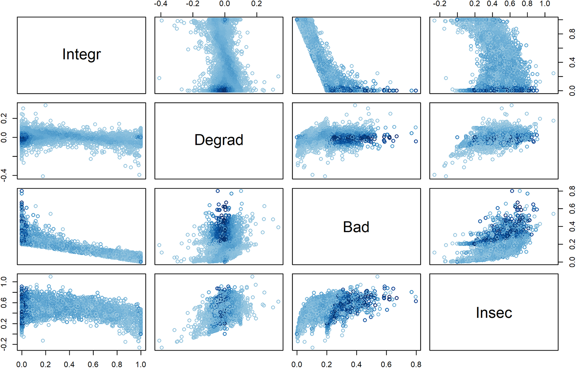
Scatter plots between quality measures for sequences of life satisfaction of elder people.
Monthly Employment Statuses
This second application illustrates how the indicators of individual sequences can serve in the analysis of employment trajectories. Employment trajectories constitute a privileged domain of application of sequence indicators. Diversity and complexity indicators have already been used in several researches to measure instability or insecurity of work trajectories (see for instance Antonini and Bühlmann 2015; Bussi 2016; Struffolino 2019; Widmer and Ritschard 2009), and the indicators that take account of the nature of the states have all been developed with the aim to analyze entry in the labor market and employment trajectories (Brzinsky-Fay 2007; Manzoni and Mooi-Reci 2018; Ritschard et al. 2018). Here, we are interested in the scarring effect of work trajectories (Abebe et al. 2016; Manzoni and Mooi-Reci 2011) and study the five-years-after impact of 36-months-long employment pathways with monthly data.
We use data from the activity calendar built from the SHP (Voorpostel et al. 2020:35-37). These are monthly data, and we consider the calendar activity sequences from September 2009 to September 2018. More specifically, to study the scarring effect, we retain the trajectories followed between September 2009 and September 2012 (three years) and look at their impact on the employment paths between October 2017 and September 2018. We restrict the study to people born after 1954 so as to exclude people who reached the legal retirement age—64 for women and 65 for men—before the end of September 2018 and retain only sequences with no missing values on the two considered periods. This leaves us with 2,407 individuals. The alphabet comprises four states: F, P, I, and U.
Table 7 reports the mean values of a selection of indicators for each of the two periods considered, that is, September 2009 to September 2012 and October 2017 to September 2018. See also Figure 5 that reports scatter plots for values of the first period. The integrative capability was computed with
Employment Sequences: Mean Values of a Selection of Indicators.
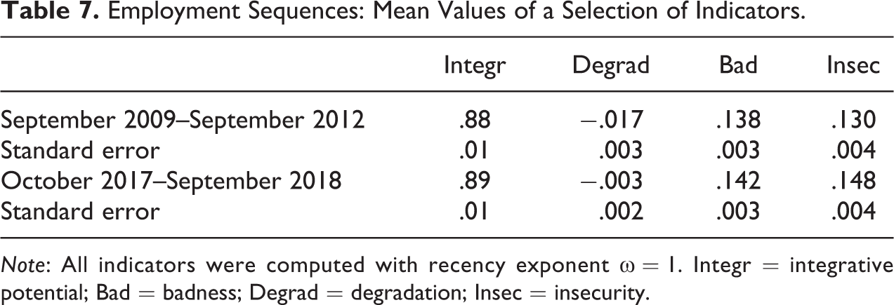
Note: All indicators were computed with recency exponent
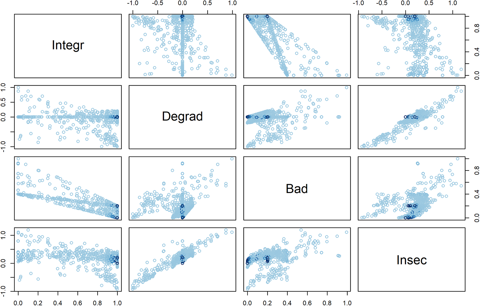
Scatter plots between quality measures for sequences of monthly work statuses between 2009-2012.
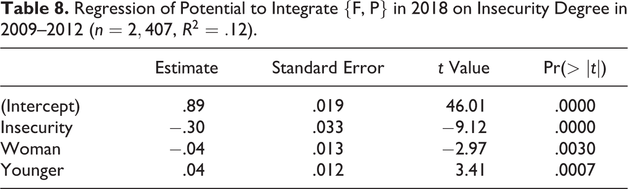
To investigate the relationship between the employment trajectory followed during the first period (September 2009–September 2012) and the path during the last observed year (October 2017–September 2018), we have regressed the capability to integrate a working status—F or P—during the last observed year on the insecurity index for the first period. The idea is to measure how the quality of the working path over 36 months impacts the degree of implication in the labor market five years later. We chose the insecurity index as an independent variable because of the multiple dimensions—complexity, degrading tendency, and undesirableness level—that it takes into account. We have introduced the sex and the age-group—youngsters born after 1975 versus elder people—as control variables. Results, given in Table 8, show a strong significant scarring effect (
Regression of Potential to Integrate {F, P} in 2018 on Insecurity Degree in 2009–2012 (
Conclusion
We have distinguished four types of sequence characteristics that can be quantitatively measured: basic features, within diversity, complexity, and quality (positiveness or badness of the sequence). Indicators of the first three types ignore the nature of the states, while quality measures require either a dichotomization of the states, for example, between states of interest and other states, or information on the undesirableness degree of the states such as a preference order. In an effort to overcome the weaknesses of some of the reviewed indicators, we have proposed novel solutions. These include a standard deviation of the spell durations that takes account of the zero time spent in nonvisited states, a revised turbulence that likewise takes nonvisited states into consideration, and three complementary quality measures—degradation, badness, and insecurity—to properly take account of the undesirableness degrees of states.
In total, we have reviewed 27 different indicators. Most of them are proportions, normalized values, or composite indexes derived from proportions and normalized values. This means that, if we exclude the nonnormalized turbulence and counts such as the length
An important issue in sequence analysis—which has no definite solution so far (Ritschard and Studer 2018b)—concerns the treatment of missing elements in the sequences. As seen above, indicators based on proportions or normalized values can straightforwardly be used with censored sequences as long as their length exceeds the alphabet size. For gaps within a sequence, two simple options can be used: treat “missing state” as a state of the alphabet or ignore the missing elements when computing the indexes. With the latter option, for instance, the integrative potential would be computed by dividing the sum of positions of the positive elements by the sum of positions of all nonmissing elements.
We will now provide some guidance for selecting indexes. The final choice will obviously depend on the data and our interest. Basic and diversity measures prove especially useful at the exploratory stage. Looking first at
For advanced studies of the arrangement within sequences, we may consider one of the composite complexity indicators—objective volatility, complexity, and revised turbulence—that combine several dimensions. Among the two indexes based on the proportion of transitions, the complexity index c is richer than the objective volatility
Regarding the quality measures, the choice depends on the assumptions we are ready to make on the state undesirableness. Among the three indicators based on a dichotomization between positive and negative states, the integrative potential
Individual indicators have several advantages. First, they provide features of a sequence that do not depend on other sequences unlike the traditional sequence analysis approach that proceeds with typologies constructed from the whole set of sequences. Second, they are quantitative, as such (i) they can easily be summarized for a set of sequences, with mean and standard deviation, for example, and used to compare groups; (ii) they can straightforwardly serve as dependent or independent variables in regression analyses; and (iii) they are well suited for time evolution analysis by means of sliding or incremental windows as shown in Pelletier et al. (2020). Here, we have illustrated the usage of individual indicators with two applications using data from the SHP. The first application compares the evolution of 15-year-long life satisfaction sequences of three age groups, and results provide some evidence of a U-shaped evolution of satisfaction along the life course. An interesting aspect of the application is that by looking at individual indicators, we were able to uncover statistically significant effects that could not be seen from index plots. The second application demonstrates how the quality measures can be used in regressions to investigate the scarring effect of earlier employment trajectories. It is important to note that these small applications only have an illustrative purpose. The research questions addressed would need a more detailed examination that is beyond the scope of this study.
Although the review has pointed out the main characteristics and compared the ranking behavior of the indicators, there remains room to further improve our understanding of the indicators in at least two directions. First, it is not always clear whether the indicator increases linearly between its minimum and maximum, and it could be very instructive to explore this by means of simulation studies in the vein of what Olszak and Ritschard (1995) have done for association measures. Second, it would also be enlightening to study how the indicators can evolve with the sequence length by exploring typical scenarios of successive sequence extensions.
Footnotes
Author’s Note
This study has been realized using data collected in the “Living in Switzerland” project, conducted by the Swiss Household Panel (SHP), which is based at the Swiss Foundation for Research in Social Sciences FORS, University of Lausanne. The project is financed by the Swiss National Science Foundation.
Acknowledgment
The author is very grateful to the three anonymous reviewers. The article has largely benefited from their careful reading and constructive comments.
Declaration of Conflicting Interests
The author(s) declared no potential conflicts of interest with respect to the research, authorship, and/or publication of this article.
Funding
The author(s) received no financial support for the research, authorship, and/or publication of this article.