Sage Journals: Discover world-class research

Abstract

It is common for social scientists to use formal quantitative methods to compare ecological units such as towns, schools, or nations. In many cases, the size of these units in terms of the number of individuals subsumed in each differs substantially. When the variables in question are counts, there is generally some attempt to neutralize differences in size by turning variables into ratios or by controlling for size. But methods that are appropriate in many demographic and epidemiological contexts have been used in settings where they may not be justified and may well introduce spurious relations between variables. We suggest local regressions as a simple diagnostic and generalized additive models as a superior modeling strategy, with double-residualized regressions as a backup for certain cases.

Keywords

county level ratios generalized additive models ecological population size

A considerable amount of work in sociology uses quantitative methods to model counts at an ecological level, such as the number of crimes, protest events, or organizations in a country, state, county, city, community area, or census tract. The lion’s share of the discussion of ecological data deals with the issues of cross-level inference (see Achen and Shively [1995] for a balanced treatment)—the attempt to use data at the ecological level to make statements about lower level (paradigmatically individual) relations. However, there is a simpler, nearly inescapable problem with the use of ecological data that has not, so far as we can tell, been appreciated in its starkness, for it suggests a wholesale reevaluation of certain research techniques. The problem arises when the units of analysis vary significantly in population size and when both the outcome (y) and the predictors (x) are strongly related to the number of individuals per unit of analysis (n) in ways that we do not understand and that cannot easily be modeled. In these cases, we cannot account for differences in population size by turning the variables into ratios or by adding a control for population size, methods that would be appropriate in many epidemiological or demographic contexts.

Yet this is accepted as current best practice: Online Appendix A lists relevant publications in the American Journal of Sociology, the American Sociological Review, and Social Forces since 2000. All the examples use one of these methods—either transformation into ratios (e.g., numbers 15, 31, and 35 in Online Appendix A) or the use of linear (e.g., 8 and 19) or loglinear (e.g., 7, 9, 11, 12, and 14) controls, or both (e.g., 3).¹ Such methods are used in studies of crimes (e.g., 1–3, 5, 16, 21–25, 27, 30, 32, 33, and 38–40), social movement events (e.g., 6, 18, 26, and 34), or membership rates (e.g., 20).

In some cases, commonly used approaches are appropriate. Obviously, if either the dependent variable or the independent variables are not highly correlated with population size, there is little reason to fear that the statistical relationship between x and y will be spurious due to confounding with n. For example, the degree of political openness of some country, judged on a scale from −3 to 3 by political scientists, may have no relation to n. Compositional diversity measures (such as a segregation index) may also be relatively independent of n. Even where such independence is unlikely, we may reasonably expect a linear relationship between n and y in cases where we have a well-defined risk set. That is, two random subsets of sizes n′ and n″ from the risk set will be expected to have counts of y that stand in the same ratio as n′ to n″. For example, let y be the number of new pregnancies observed in a month, and n the number of women in the unit, then 0 ≤ y ≤ n. For this reason, we often feel confident comparing units not in terms of y but in terms of the ratio r = y/n. This might be especially true when we are interested in the effect of some independent variable x which also has a theoretically well-defined relation to this risk set. For example, we might be interested in the number of women in any unit who are employed. We might therefore regress y/n on x/n without any complications (assuming independence of units, no threshold effects, etc.).²

However, this is only a subset of all the types of situations in which we have good reason to expect that both x and y are strongly related to n. In many other cases, we cannot be confident that we have a clearly defined risk set, although we still expect the predictors and dependent variable to be related to n. For example, in a time of widespread protest, although we might expect larger areas to have more protest events, we do not think that each individual is “at risk” of initiating such an event. This situation, if uncorrected, would lead to Type I errors—the analyst rejecting the null hypothesis of no relation between x and y when, in fact, x and y are independent conditional on n. If we have no clear way of specifying the nature of either of these relations (x-n and y-n), we cannot predict, in advance, the pattern of data that should be implied by a null hypothesis. In these cases, even minor model misspecifications can lead to misleading results.

Sociologists dealing with longitudinal data are familiar with a similar problem. They are used to analyzing series of data (e.g., data on national economic trade patterns and median population wealth) in which all the analyzed variables tend to be bound up with the time of the observation. No one doing such analyses would rely on a simple linear control for time as a way of addressing this issue. Instead, scholars often go to elaborate lengths to purge their data of nonstationarity before conducting multivariate analyses. Yet, we have relied on such simple linear controls for count data and population size, as our survey of the literature indicates.

This article proceeds as follows. We first diagnose the problem and discuss it in more detail using a combination of real-world data and simulations. We then propose a simple diagnostic technique to check whether an independent variable is a valid predictor of the dependent variable, even net of population size. Finally, we suggest superior estimation strategies, test their applicability, and discuss limiting cases.

The Problem

Data Example

Let us take the case in which y is a count of organizations or events, which we hope to relate to some x which is a similar count. Say, for example, that we are interested in the relationship between the strength of a social movement and the strength of religious organizations. It has often been noted that political movements draw their capacity to mobilize from preexisting organizations, in many cases churches (see Morris [1984] for the Civil Rights Movement). As a running example, we take the case of the Tea Party movement and ask whether the movement produced more events in areas where there were more evangelical churches than in areas that had fewer of these preexisting organizations.

Figure 1 shows data on the relationship between the number of evangelical churches and the number of Tea Party events in the U.S. counties from June to Election Day 2010.³ The top panel gives the relation in raw form; the bottom panel presents the relation between the logarithms of both counts. As can be seen, there is a strong positive relation between the two variables. Model 1, Table 1, is a bivariate linear regression which confirms this positive relation.⁴ The problem is that such a relation should be expected even if there is no true effect of churches on events. Simply put, we should expect that places with more residents will have both more churches and more events. The raw correlation, in other words, cannot be used to test the null hypothesis of no relation between the two variables. Somehow, we need to purge the relation between our variables of the common covariance due to population if we are to see whether there is something about the presence of evangelical churches, and not the mere population size, that predicts Tea Party events.

Figure 1.

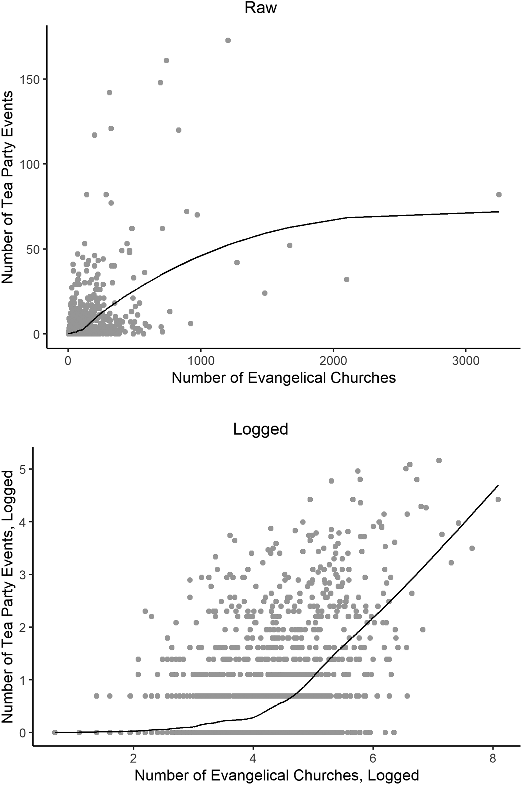
Tea Party events by evangelical churches, county level. Note: The curves show loess fits with span = .3 and degree = 2.

Table 1.

Models for Number of Tea Party Events, County Level.

Panel A
OLS and Shape Constrained Gaussian GAM With Identity Link Function
	Model 1	Model 2	Model 3	Model 4	Model 5
Model	OLS	OLS	OLS	OLS	GAM
Approach	Naive	Ratio	Control for n	Ratio + n	Monotonic
Churches	.041***	−0.005***	0.009***	−0.004***	−0.001
	(.001)	(.001)	(.003)	(.001)	(0.003)
Population			0.013***	<0.0001	Smoothed
			(.001)	(<.0001)
Constant	−.584***	0.020***	0.081	0.019***	−2.165
	(.157)	(.002)	(.163)	(.002)	(1.750)
Observations	3,114	3,114	3,114	3,114	3,114
R ²	.277	.007	.311	.007	.366
Panel B
Poisson, Negative Binomial, and Shape Constrained Poisson GAM With Log Link Function
	Model 6	Model 7	Model 8
Model	Poisson	Negative Binomial	Poisson GAM
Approach	Control for n	Control for n	Monotonic
Churches	.002***	0.005***	<0.0001
	(.0001)	(.001)	(<.0001)
Population	−.0002***	0.005***	Smoothed
	(<.0001)	(.0004)
Constant	.412***	−1.042***	−21.578
	(.014)	(.062)	(.356)
Observations	3,114	3,114	3,114
Deviance explained	.167	.317	.579

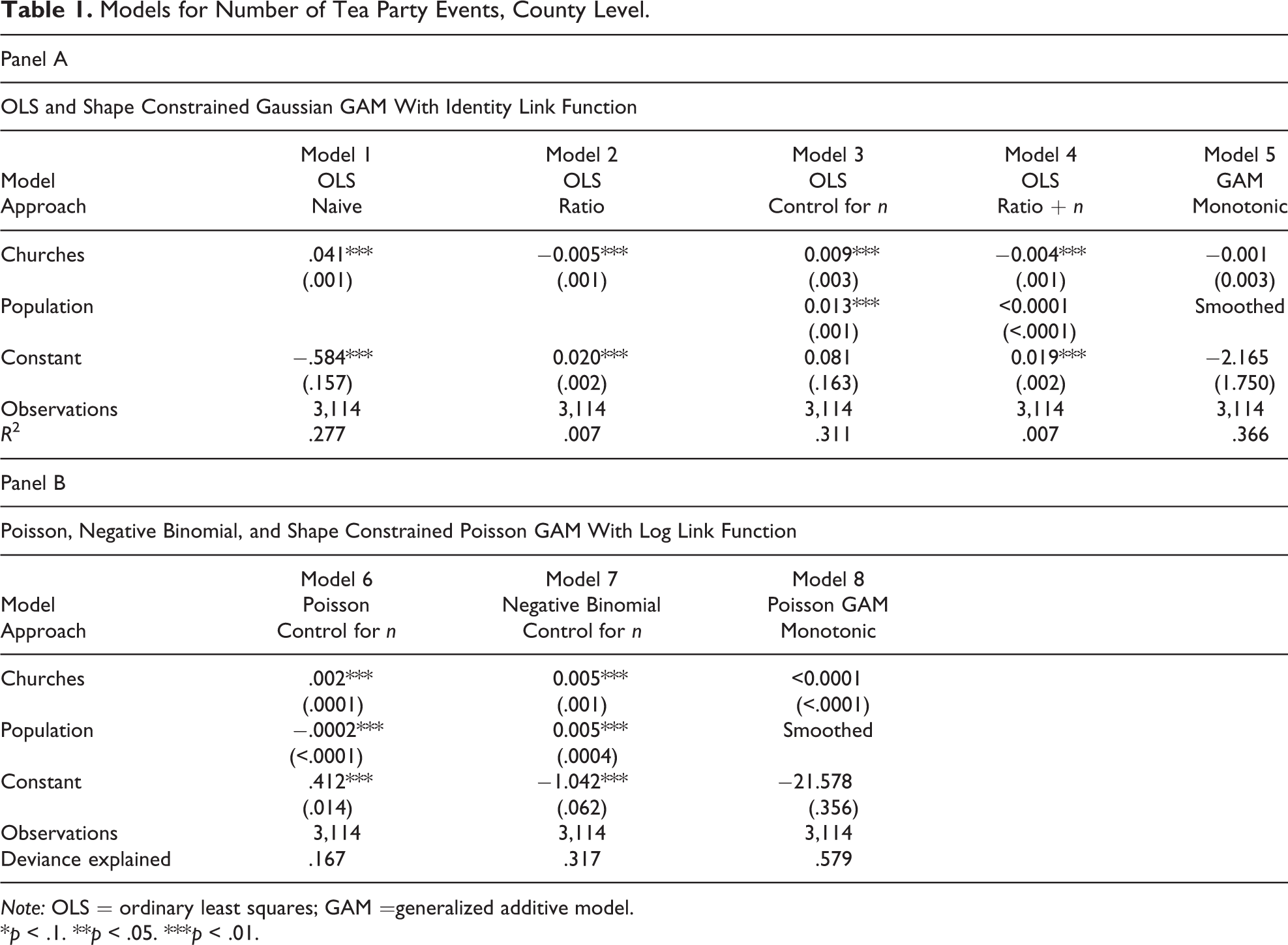
Note: OLS = ordinary least squares; GAM =generalized additive model.

*p < .1. **p < .05. ***p < .01.

Perhaps our problem is that we should not be looking at the sum of total events and total number of churches but the events-per-person and churches-per-person ratios. Model 2, Table 1, shows the results of regressing Tea Party events per person on evangelical churches per person. Again, the relationship is highly significant. But now it is a negative relation. This might seem surprising. Perhaps even more surprising are the results when we replicate, only now, instead of using ratios, regressing Tea Party events on the number of churches in each county, but controlling for n (model 3, Table 1). Here, we see that the relation is positive, and again, statistically significant.

We might not initially expect such a radical difference between the results of these two models, given that model 2 fits

\frac{y_{j}}{n_{j}} = b \frac{x_{j}}{n_{j}} + c + ε,

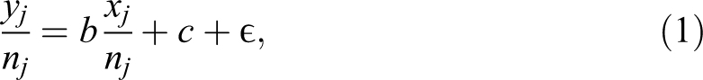
while model 3 fits

y_{j} = b^{*} x_{j} + c^{*} n_{j} + q + ε^{*},

where J is the number of units, the * indicates that the parameters in equation (2) are different from the corresponding ones in equation (1), and q denotes the new intercept in equation (2). It seems that in equation (2), we have merely multiplied equation (1) by n_j, which would change nothing. But the two equations are not the same; equation (2) has three free parameters and equation (1) only two. For this reason, it has been recommended that analysts include a term of (1/n_j) when fitting the ratio model or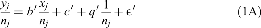

\frac{y_{j}}{n_{j}} = b^{'} \frac{x_{j}}{n_{j}} + c^{'} + q^{'} \frac{1}{n_{j}} + ε^{'}

(Firebaugh and Gibbs 1985). Yet even with this correction, neither equation (1) nor (1A) will estimate the same slope of x on y as will equation (2) if the actual relations between y and n on the one hand and x and n on the other hand are not linear (this is demonstrated in more detail in Online Appendix B). For the case at hand, adding such a term (not shown, though part of our provided code) gives us nearly the same coefficient as does model 2.

Because equation (2) has one more free parameter than does equation (1), we might think that the results of model 3 are more robust than those of model 2 and that this model produces the correct estimate of the relation between evangelical churches and Tea Party events. But, given the fact that the ratio and the control model have opposite signs, we might suspect that the two methods may have compensating biases. For this reason, we might think that the most conservative approach would be to do both at once. Model 4, Table 1, shows that doing this, by adding population as a control to the ratio model, really makes no difference, as it gives the same results as the ratio model (and not, as we might have guessed, the more flexible model 3). For this reason, we might now suspect that the ratio model is correct, as it seems to have successfully purged our data of confounding by n. Certainly, we cannot decide which model to prefer by looking at explained variance, for in many cases (although not for the example discussed here) the explained variance will be greatest for equation (1), which has the effect of n on both sides of the equation.

We have, in sum, two very different interpretations of the data: In one, there is a strong positive, and in the other, a strong negative relation. Neither interpretation is justified, as we will go on to show. (To anticipate, a null effect is found in model 5, Table 1.) There is no reason to think that the number of evangelical churches has any relation to the number of Tea Party events that is not a result of population size. In other words, neither technique works to test the null hypothesis of no relation, and we believe that, for this reason, it is likely that similar work has also falsely rejected the null hypothesis when it should not be rejected.

How can this be? The answer is that in both techniques, too much rests on the linearity assumption. While there is good reason to believe that both our dependent and our independent variables covary strongly with population, there is no reason to think that this covariation is linear. Such a combination of strong but nonlinear effects means that both techniques do not remove the confounding due to n, but in fact, can actually increase it. We go on to demonstrate this with a set of simulations.

Simulation Example

We begin by showing how nonlinear relations between variables and population size produce false relations between predictors and dependent variables. We conduct simulations as opposed to using real data because we can be sure that there is no true relation between our dependent variable and our predictors. We sample J = 1,000 observations for n from a uniform distribution⁵ and generate four variables as follows: $y = n^{.25} + ε_{y}$ , $x_{1} = n^{1} + ε_{x_{1}}$ , $x_{2} = n^{3} + ε_{x_{2}}$ , and $x_{3} = n^{.25} + ε_{x_{3}}$ , where the errors are normally distributed with means of zero and variances proportional to n to the power of 0.25, 1, 3, and 0.25, respectively. All variables are thus conditionally independent given n. We first scale all variables, so that their minimum is zero to ensure nonnegative values, before creating ratio versions (e.g., x₁/n) and rescaling those to have a mean of 0 and a variance of 1 to simplify parameter interpretation. Model 1, Table 2, gives the naive regression corresponding to model 1, Table 1. It should be noted that in model 1, the relation between x₂ and y is not significant. This is because with one variable (y) scaling strongly with n at an exponent much less than one (we shall call these “sublinear effects”), and the other (x₂) with a coefficient much greater than one (we shall call these “supralinear effects”), the pattern is so nonlinear that the linear slope is quite small.

Table 2.

Simulated Data.

	Model 1	Model 2	Model 3	Model 4
	Naive	Ratio	Control for n	Ratio + 1/n
x₁ (∼n¹)	.307***	.439***	.019	0.937***
	(.030)	(.034)	(.035)	(.032)
x₂ (∼n³)	−.023	.292***	−.234***	1.765***
	(.022)	(.039)	(.026)	(.064)
x₃ (∼n^.25)	.663***	.186***	.423***	0.480***
	(.023)	(.024)	(.028)	(.022)
n			.702***
			(.054)
1/n				−2.104***
				(.080)
Constant	.000	−.000	.000	−0.000
	(.012)	(.019)	(.011)	(.015)
Observations	1,000	1,000	1,000	1,000
R ²	.846	.635	.869	.785

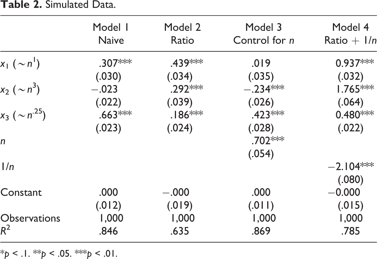
*p < .1. **p < .05. ***p < .01.

Model 2, Table 2, presents the results when we turn all our variables into ratios, corresponding to model 2, Table 1. The ratio model likewise does not correctly identify null relations.⁶ Model 3, Table 2, employs a control for population corresponding to model 3, Table 1. Adding the control for population works to eliminate the spurious significance of the variable that scales linearly with population (x₁). But it does not identify the spurious relations of y with the other predictors. Indeed, we now see a significant negative relation between y and x₂ where this was not present in the naive model. Model 4, Table 2, follows Firebaugh and Gibbs (1985) and adds (1/n) as an additional control to the ratio model. Far from this technique correctly leading us to accept the null hypothesis for our coefficients, the estimates are all larger than in the simple ratio model.

In sum, even the flexibility of the control model, which allows for any linear relation, is not sufficient to remove false positive findings if the true relations are not linear. Of course, it is always true that an improperly specified functional form means that our model results are misleading. What is important about the set of cases discussed here is that we have extremely good reasons to believe that many of the variables of interest are strongly dependent on n, but that there is no reason that these relations should be assumed to be linear, or even of any form that can be specified in advance (for work on the different functional forms relating various aggregate variables to size, see Bettencourt et al. 2007; also Bettencourt 2013).

One response to this, taken in some kindred fields, has been to treat the scaling of any variable as an empirical matter. Here, one usually proposes that the true relation between some variable x and n takes the form

x = q (n^{a}),

and constructs

ln (x) = a ln (n) + l n (q) .

We can estimate a either by fitting equation (3) directly or by fitting equation (4) as a linear model (the results, however, will generally be different; see Petersen 2017; also Stolzenberg 1980:460-63). We thus generalize from a linear relation to a power law.

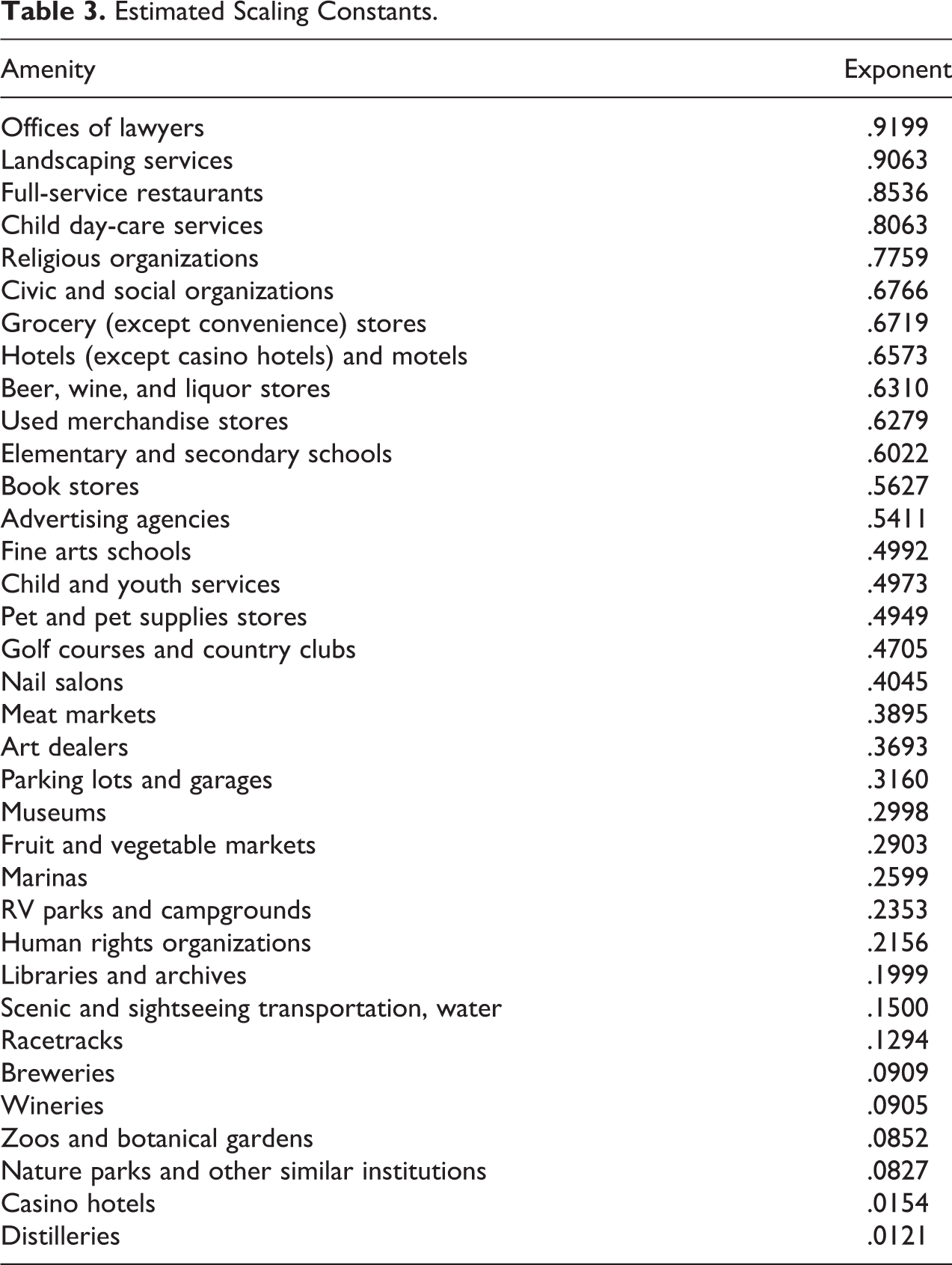
For an example, Table 3 gives estimates of the exponent linking the number of the amenities in any U.S. county to the number of residents of this county.⁷ On one extreme, the number of lawyers or landscapers scales nearly linearly with population. On the other hand, the number of distilleries grows quite slowly with population. It is worth emphasizing that these relations are nonlinear enough to lead to spurious conclusions with rather moderate sample sizes. To illustrate this point, we create two variables, one that scales with n at the level of marinas and another that scales with n at the level of fine arts schools (see Table 3). We find that if we regress one on the other using a control for n, we would wrongly reject the null hypothesis around half the time when the number of cases is around 250; if we use a ratio approach (whether or not we add a term for 1/n), we would reach this point at around 50 cases (and there are in fact 3,073 counties in these data).⁸ Of course, if these estimates of the exponents could be relied upon, we could adjust any regression involving them accordingly. However, what we need is not the marginal distribution of some x against n, but the structural relation that would allow us to correctly estimate various regression coefficients. We cannot estimate such exponents unless we already know the coefficients linking the independent to the dependent variable.

Table 3.

Estimated Scaling Constants.

Amenity	Exponent
Offices of lawyers	.9199
Landscaping services	.9063
Full-service restaurants	.8536
Child day-care services	.8063
Religious organizations	.7759
Civic and social organizations	.6766
Grocery (except convenience) stores	.6719
Hotels (except casino hotels) and motels	.6573
Beer, wine, and liquor stores	.6310
Used merchandise stores	.6279
Elementary and secondary schools	.6022
Book stores	.5627
Advertising agencies	.5411
Fine arts schools	.4992
Child and youth services	.4973
Pet and pet supplies stores	.4949
Golf courses and country clubs	.4705
Nail salons	.4045
Meat markets	.3895
Art dealers	.3693
Parking lots and garages	.3160
Museums	.2998
Fruit and vegetable markets	.2903
Marinas	.2599
RV parks and campgrounds	.2353
Human rights organizations	.2156
Libraries and archives	.1999
Scenic and sightseeing transportation, water	.1500
Racetracks	.1294
Breweries	.0909
Wineries	.0905
Zoos and botanical gardens	.0852
Nature parks and other similar institutions	.0827
Casino hotels	.0154
Distilleries	.0121

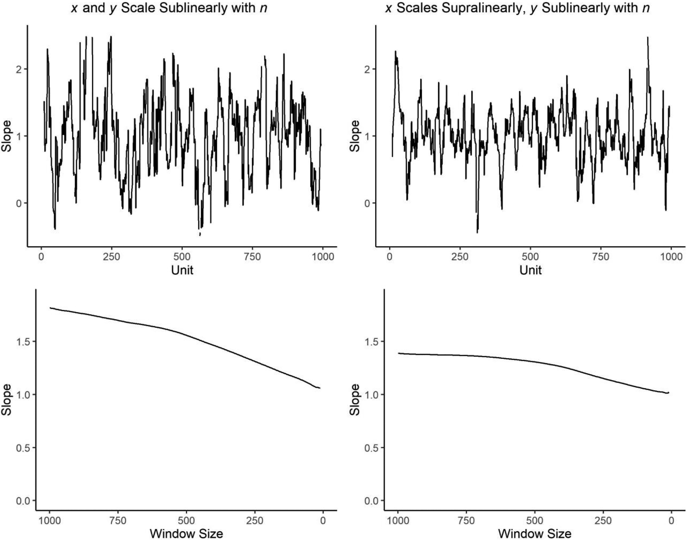
Still, if the relation between these x’s and n were quite strong (with high predictive power), we might feel confident in using the observed relation between the two (as in Table 3) as an estimate of the structural coefficient. However, these relations in many cases will be noisy. Even when the fit in a logarithmic metric is rather good (Figure 2, top left, for lawyers; the value of the estimated coefficient a is given in the bottom right corner of each plot), we see that the explained variance is low on the right side of the untransformed data curve (Figure 2, top right), as most observations tend to be on the left. With cases that scale sublinearly (Figure 2, bottom left and right), the relations are even more inexact. The empirically fit line therefore has a tendency to produce large residuals at the right tail, which then become outliers that can lead to misleading results. The fact that the observations are clustered at the left tail, where the power-law relation tends to break down, also leads to a discrepancy in estimates depending on whether we are using the log or the linear metric.

Figure 2.

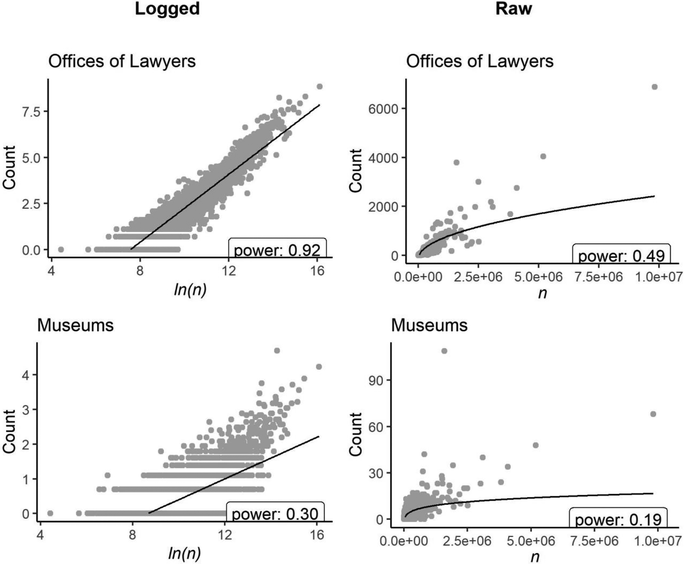
Empirical relations, amenities by county.

For this reason, we go on to propose a more flexible approach that has two prongs. The first is one of diagnosis, in which we attempt to determine whether or not we are safe in rejecting the null hypothesis of no effect of x (or of multiple x’s) on y. Second, we go on to suggest two ways of attempting to quantify the effect of x on y given an unspecified relation of both with n. The first approach, which uses a double-residualized locally smoothed regression, is extremely conservative, which makes sense: Given the demonstrated tendencies for false positives in such data, we believe it is important to err in the other direction. However, we also suggest the use of generalized additive models (GAMs) which, we demonstrate, perform well in a wide variety of situations (though not all).

Techniques for Analysis

Diagnosis: Local Effects

If one of our independent variables x really is a valid predictor of the dependent variable y (let us assume a positive slope), even net of n, we should expect to find positive relations between x and y in subsets of the data that are similar in their n. Thus, the simplest diagnostic procedure is to stratify the data by n, take subsets of the data (“windows”) that are similar in n, and examine the proportion of such windows that have a positive relation between x and y. Where this proportion is not large, we should refrain from attempting to model the relation of y and x.

The graphical representation of these local relations, however, can be more enlightening than the sheer percentage count. Figure 3 shows the effects for x₁, x₂, and x₃ from local regressions applied to the simulated data used in Table 2, where we order the cases by n and then run our regression of y on x₁, x₂, and x₃ with a moving window of nine cases. If there was a positive (negative) effect for some variable, we would expect the line corresponding to its local slope to spend more time above (below) the zero point than below (above). Instead, all lines show very little order. This is quite different from a case in which the relation between y and x tends to be positive at one end of the scale and negative on the other, despite this leading to a similar overall statistic. In such a case, we might believe that there was a true connection between y and x, though one that differs by unit size. In the case at hand, however, we seem to have a strong signal of no relation (and this is of course quite correct).

Figure 3.

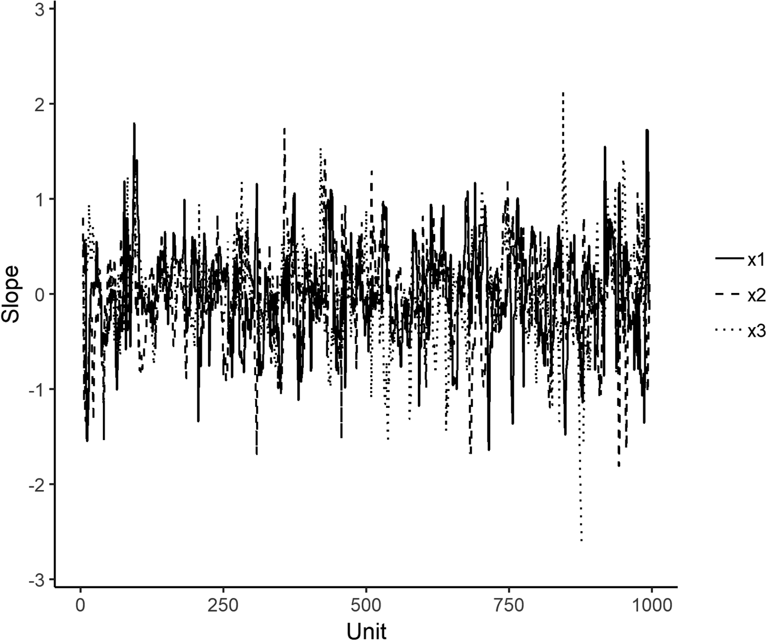
Local regression effects, simulated data with true effect = 0.

One might worry that a small window leads to estimates that are too unstable to be of use; on the other hand, a large window will have too much variation in n to provide a good test. One way to avoid erring on either the side of too large or too small a window, then, is to determine whether any local slope goes steadily toward zero as the width of the moving window decreases. Figure 4 gives the results of the average slope for the same x₁, x₂, and x₃ analyzed above when we successively decrease the size of the window from the full original data (which is equivalent to the global model) to a minimum of seven. As we can see, there is a clear trend toward effects of zero as the window gets smaller. This again suggests that we should not reject the null hypothesis of no relation. Where the results of the diagnostics are as clear as these, we would believe there would be no reason to pursue an investigation of the effect of x on y.

Figure 4.

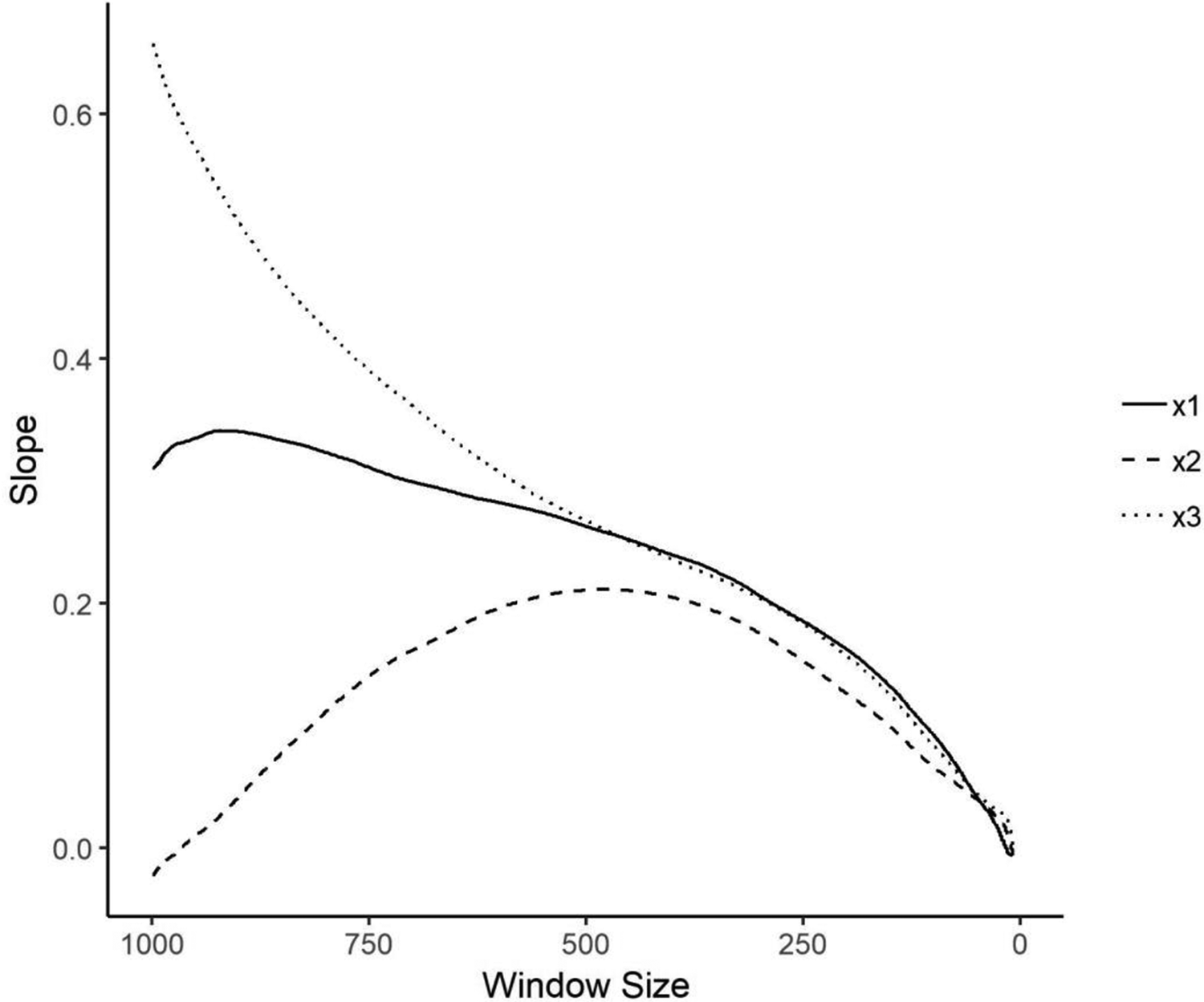
Effects of moving window size, simulated data with true effect = 0.

Replicating Figure 3 with a moving window of size 15 for our case of the relationship between Tea Party events and the number of evangelical churches (results not shown), we find that in 37 percent of the windows, the slope of events on churches is positive, and in 63 percent, it is negative. Although the proportion of negative cases is substantially larger than 50 percent, we do not see an interpretable pattern such as a change from a zero relation to a negative one at larger or smaller windows, such that we could accept the fact that the relation is usually, though not always, negative as theoretically significant. More important, Figure 5 replicates Figure 4 for the Tea Party events data and sees a steady decline in the value of the estimated effect. As we can see, we have little reason to believe that in fact there is any relation between the number of churches and the number of events that is not easily explainable by n.

Figure 5.

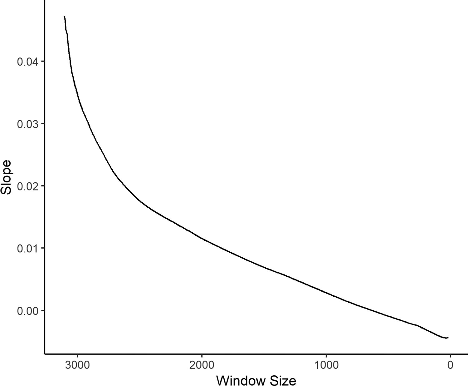
Effects of moving window size, Tea Party events.

To demonstrate the capacity of this technique to correctly identify nonzero associations, however, we need data in which we know the real relation between x and y. Let us develop a general framework for simulating data from two variables, each of which is related to n in a nonlinear way. Let

x = f_{1} (n) = c_{x} + b_{x n} n^{a} + ε_{x},

and

y = f_{2} (n, x) = c_{y} + b_{y n} n^{d} + b_{y x} x + ε_{y},

where

ε_{x} \sim N (0, σ_{x}),

and

ε_{y} \sim N (0, σ_{y}) .

Here, we produce two simulated data sets, in both of which there is a true relation between x and y independent of n (b_yx = 1.0). In the first, both x and y scale sublinearly with n ( $a = d = .3$ ), and in the second, y scales sublinearly with n, and x supralinearly (a = 2, d = .3). In both cases, we set b_xn = b_yn = 1, σ _x = sd(n^a)/3, and σ _y = sd(x + n^a)/3. We adjust c_x and c_y such that min(x) = min(y) = 0. Figure 6 displays the diagnostic plots corresponding to Figures 3 and 4 for these two cases of simulated data. For the first case, 95 percent of the moving windows are positive; for the second case, 99 percent are positive (see Figure 6, top). Figure 6, bottom, shows that the local estimates of b_yx tend to be too high when the windows are large, but they decrease toward the true relation as the windows become smaller, and they do not make a beeline for zero as do the cases in which there is no true relation. Figure 6, then, indicates the sort of results that would suggest that we cannot rule out a direct relation between x and y.

Figure 6.

Local regression effects and effects of moving window size, simulated data with true effect = 1.

While these simple techniques seem surprisingly effective at indicating the magnitude of an effect, in addition to indicating whether it is likely to be zero, these are still rule-of-thumb procedures and give us no way of properly estimating the size of the coefficients and the standard errors. We go on to propose two different approaches to this task.

A Two-stage Approach

As we noted above, the problem with the commonly used techniques to determine the effect of some x on y independent of n, including that which fits a power-law distribution, is that deviations from the assumption of the functional form relating n to y may be consequential, given that many independent variables will also increase with n in a hard-to-predict way. We therefore propose that rather than divide the observed counts by n or include a function of n as a control, we residualize them on a smoothed curve of y on n. Thus, we replace y with y* = y − f(n).⁹

Of course, the results are likely to be somewhat sensitive to the degree of smoothing used. Further, such a curve might at some points head downward (i.e., the predicted y decreases locally with increases in n), which goes against the core assumptions motivating our concern. We take for granted that there are a number of unmeasured processes all of which mean that counts of our variables will tend to be higher in units with larger n, even though the relation is likely to be nonlinear, perhaps even discontinuous. Certainly, we have no reason to imagine a negative relation between these processes and n. For this reason, we propose adjusting any algorithm used for such smoothing so that it is monotonically nondecreasing. Several algorithms for monotonically increasing smooths have been put forward.¹⁰ We use shape-constrained B-Splines as proposed by Ng and Maechler (2007) and implemented in the R package cobs. Note that in some cases, a smoothing routine will perform better if applied to y on a log scale than a linear scale; we would recommend doing both and choosing the more conservative results.

We would then be interested in the regression coefficient in a model regressing y* on x or on additional predictors (such an approach has been taken to dealing with spurious correlation induced in temporal series data by Fischer and Hout [2006:252-56]). However, such residuals y* may lead to biased estimates, by taking out of y all the covariance with x that overlaps with the shared covariance with n (Freckleton 2002). Accordingly, there are two techniques that have commonly been suggested to correct estimates of b_yx derived from models linking y* to x. The first is to include n on the right side, thereby soaking up the effect of the removed common covariance, and the second is to residualize x on n as well, and model y* = x* + c (we shall call this model “double residualization” [DR] henceforward). While these two techniques lead to similar results where the true relations are linear, in cases where x or y is a nonlinear function of n, we show that the latter is superior.

To demonstrate the utility of this technique, we need data for which we are sure that the true relation between x and y is zero. To create such data, we take the Tea Party data on U.S. counties used above and construct a variable x following equation (5). We vary a, the exponent linking n to x, and set b_xn = 1 and σ _x = sd(n^a)/3. Because we want to examine the performance of ratio models, we also want our x to be strictly nonnegative. We therefore adjust c_x such that min(x) = 0. By construction, we set x to be unrelated to y conditional on n (b_yx = 0 in equation [6]). We then use this constructed x to predict y, which in this case is the observed number of Tea Party events held in some county. Table 4 contains results in which the columns represent seven models linking y to x. The first column is the result from the naive regression, y = f(x), the second is from the ratio model (equation [1]), the third is from the model that controls for n (equation [2]), the fourth is from the ratio model that includes (1/n) as a control (equation [1A]), the fifth is from the regression of y* on x (“single residualization” [SR]), the sixth is from the regression of y* on x that also includes n as a predictor, and the seventh is from a regression of y* on x* (DR). The values in any cell are the percentage of trials (out of 500 done for each value of a) in which the null hypothesis was rejected at p < .05.

Table 4.

Percentage (False) Rejection of H₀, Simulated Tea Party Data.

	Model 1	Model 2	Model 3	Model 4	Model 5	Model 6	Model 7
a	Naive	Ratio	Control for n	Ratio + 1/n	SR	SR + n	DR
0.25	100	100	100	87.8	100	100	4.8
0.5	100	96.6	100	31.6	100	100	4
1	100	90.6	4.8	15.2	100	5.2	4
2	100	91.4	100	18	100	100	5.8
4	100	92.4	100	15.6	0	100	15.4

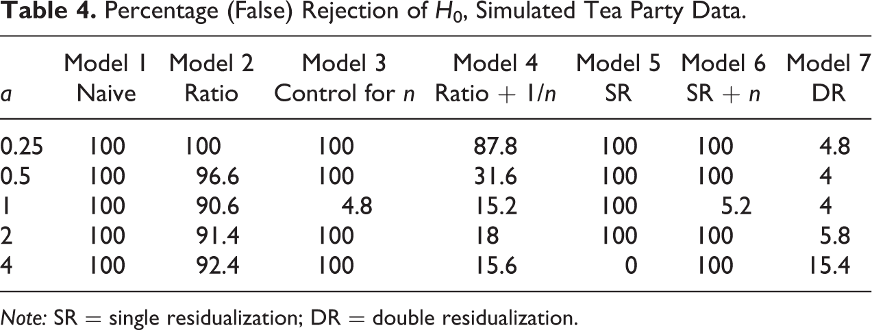
Note: SR = single residualization; DR = double residualization.

As expected, in the case where x is a linear function of n ( $a = 1$ ), either controlling for n (model 3) or SR plus a control for n (model 5) rejects the null hypothesis around 5 percent of the time—just what they should do with a p < .05 test. But while the other techniques tend to fail for cases in which the exponent is not equal to 1, DR works rather well, only breaking down at extreme exponents.¹¹

This suggests that DR is good at failing to reject the null hypothesis when in fact it is correct. This does not, of course, mean that it is useful in correctly estimating the effect of x on y when this effect is nonzero. Figure 7 displays the results of simulations in which we use equations (5–8) to generate data in which both x and y are strongly influenced by n, but there is a true relation of x on y conditional on n. We set b_xn = 1, σ _x = sd(n^a)/3, and σ _y = sd(b_ynn^d + b_xnx)/3. We choose b_yn such that var(b_ynn^d) = var(b_xnx), making sure that x and n contribute equally to y across simulations. Finally, we adjust c_x and c_y such that min(x) = min(y) = 0. Each layer represents one particular value of b_yx, with the two dimensions of any layer being the exponent a linking n to x (on the vertical) and the exponent d linking n to y (on the horizontal). The value displayed via the coloration is the average of the absolute value of the percentage error of the estimated coefficient, that is, the average of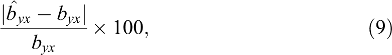

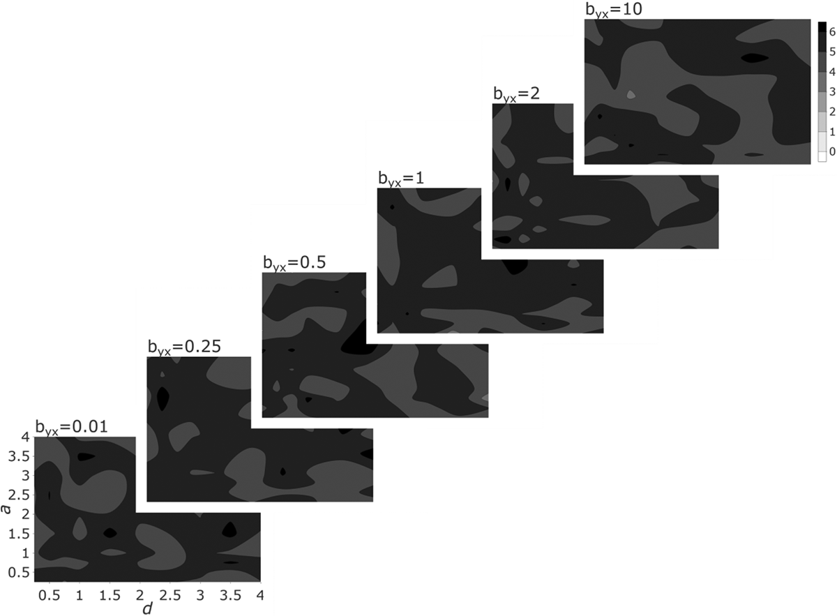
\frac{| {\hat{b}}_{y x} - b_{y x} |}{b_{y x}} \times 100,

computed over 50 simulations for each value of a, d, and b_yx.¹² The darker the value, the higher the error.

Figure 7.

Estimation error of double residualization. Note: The contour plots show the absolute value of the percentage error, $\frac{| {\hat{b}}_{y x} - b_{y x} |}{b_{y x}} \times 100$ , averaged across 50 simulations.

As we can see, the method produces estimates that are close to the correct value of b_yx across a wide range of parameter values. Further, the error is much lower than that produced by SR or SR and the inclusion of n as a covariate. Figure 8 demonstrates this by overlaying three distributions: (a) the distribution of percentage error by SR, (b) that of SR and a control for n, and (c) that of DR. The difference between the mean of any distribution and zero indicates the bias of that technique and the width of the distribution the degree of error. DR is the only technique that is unbiased, and its error is reasonably low.

Figure 8.

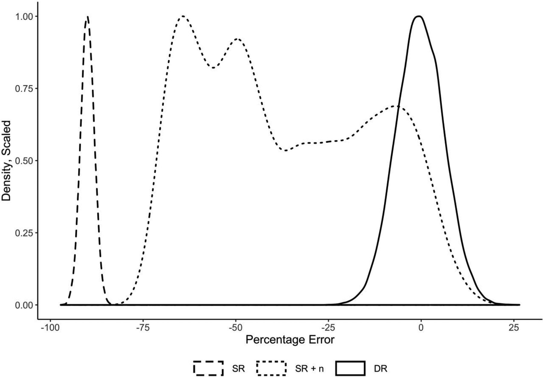
Comparison of error densities, three modeling approaches. Note: The densities were scaled to a maximum of 1. The error is defined as $\frac{{\hat{b}}_{y x} - b_{y x}}{b_{y x}} \times 100$ .

Limitations

DR, then, seems to work reasonably well at estimating coefficients from simple models. There is, however, an important limitation. This method, based on residualization, only works where our variables are reasonably normally distributed—most importantly, where y >> 0. But in many cases of aggregate data, our dependent variables are counts that are on the order of 0–10. In particular, we often have many cases of relatively small n and fewer of large n, which means that we have many cases in which the dependent variable is quite small. In such cases, no method that relies on residualization can be expected to work correctly (see, e.g., Angrist and Pischke 2009), as we will tend to have many impossibly negative predictions for the cases with small n’s. For these reasons, we go on to propose and investigate the application of semiparametric models that may be used with Poisson distributed data.

GAMs

Here, we adopt a semiparametric modeling approach known as GAMs (Hastie and Tibshirani 1986, 1990; Hastie, Tibshirani, and Friedman 2009:295-304). Such models combine conventional parametric prediction with nonparametric prediction. The nonparametric aspects may be conducted via a number of different methods including loess smoothing and various forms of spline functions. In other words, given some nonparametric function f of n, we estimate the model

E [y | X, n] = g (β X + f (n)),

where g() is some link function, X is a matrix of covariates (including the 1-vector if we wish to add a constant), and β is a vector of estimated coefficients.

It was this method that was used in Table 1, model 5—the model that did not reject the null hypothesis. While models 1 and 3 produced a significant positive effect of the number of churches on the number of Tea Party events and models 2 and 4 produced a significant negative effect, only the GAM suggested that we should not actually reject the null hypothesis of no relation between the two variables. As indicated by our diagnostics, the GAM was correct in not rejecting the null hypothesis.

It will be noted that when g() is the identity (linear) function, this model becomes

y = β X + f (n),

which is quite similar in expression to the model for the residuals, namely

y - f (n) = β X .

The difference lies in the simultaneous estimation of f() and β in the GAM. But there is a more important advantage of the GAM: We are not restricted to a linear link function. Given that our concern is that we may have a dependent variable that is a count that must be nonnegative, we here use Poisson models that are restricted to nonnegative integer prediction.¹³ Again, we constrain the relationship between y and n to be monotonically increasing and estimate so-called shape constrained GAMs with monotonically increasing P-splines as smooth functions (see Online Appendix C for more details). Here, we simulate data so that the amount of variation in y coming from our independent variable and from n is constant across simulations, while we vary the mean of y. Given a distribution of n that is log-uniform, and given exponents a and d as defined above, we begin by producing x as follows:

x \sim P o i s s o n (μ_{x}),

where

μ_{x} = n^{a} / λ,

and choose λ such that the average $μ_{x}$ is 1.5. We then construct

y \sim P o i s s o n (μ_{y}),

where

μ_{y} = exp ([b_{y x} x + ω (n^{d})] / 10^{β}) .

Because of the logarithmic link in the Poisson model between the outcome and the predictors, we make the formula for μ _y take an exponentiated form of the n term. To compensate for the increased scale, we then divide by 10^β where β is a tunable parameter chosen so as to give us the desired mean of y. We choose ω such that

v a r (ω (n^{d})) = v a r (b_{y x} x) .

In other words, we try to make sure that x and n are contributing the same degree of variance in y across simulations. We here use a = d = .3 and b_yx = 2.

Figure 9 displays the results of simulations in which we vary the mean of y. For each method (GAM and DR), we display a line showing the average error (the bias) over 50 simulations, as well as surrounding lines indicating where the 25th and 75th percentiles of estimates lie. The distribution for the GAM is shaded and uses solid lines; that for the DR is unshaded and uses dashed lines. We can see that as the mean of y goes down, the error rises both for the double-residualized estimates and for those of the GAM. The GAM, however, performs well until the mean gets quite small and continues to have somewhat smaller errors at the lowest values of y.

Figure 9.

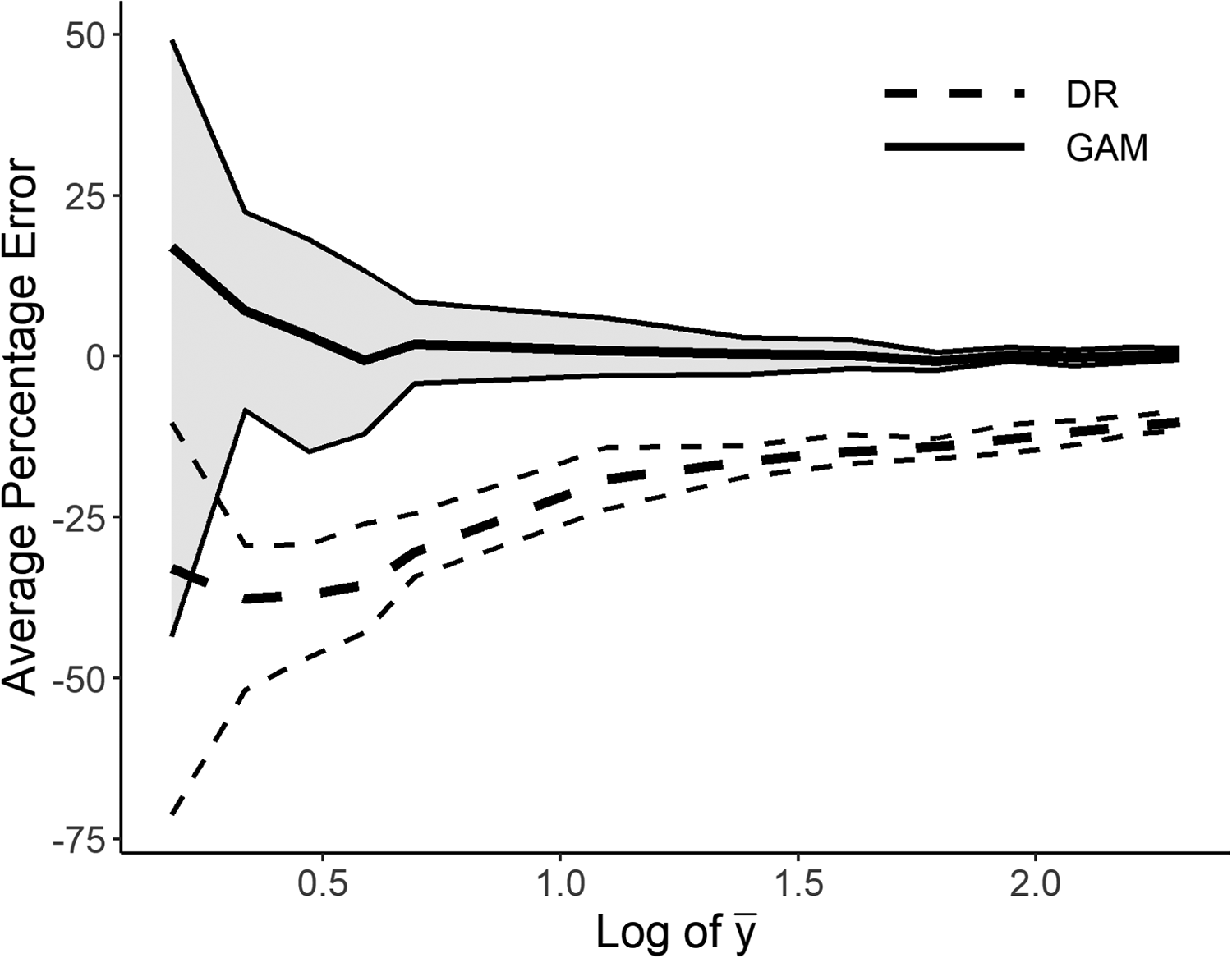
Comparison of average degree of error, double residualization, and generalized additive model. Note: Average percentage error (thick line) as well as the 25th and 75th percentile of the errors (thin lines). We drop values of mean(y) smaller than 1.2 because the variance of the errors gets very large, making the graph illegible.

Given that such a modeling approach seems to solve all our problems in one fell swoop, it may be asked why we should proceed with the DR model at all, as opposed to recommending the GAMs in all instances. First, there are extreme cases (illustrated in our provided code) in which the GAM is more likely to incorrectly reject a true null hypothesis than is the DR technique.¹⁴ Second, the method of DR can be used to fit more complex models that cannot now be combined with the GAM, models that are likely to be of interest to scholars using aggregate data that come from areal units. Double-residualized methods could be combined with autoregressive (Anselin 1988) or nonstationary (Congdon 2006) models for spatially located data. We leave this for further exploration.

Conclusion

Some may respond to the critique offered in this article that since all of our models are wrong, and we must always simply hope that we have a reasonable specification, it is unfair to pick on certain types of analyses to be held to a higher standard than others. We have two responses to this objection. First, when it comes to aggregate data in which n varies across cases and puts some constraints on the distribution of both independent and dependent variables, we have good reason to think that our models have extremely high degrees of nonlinear interrelations, such that forms of misspecification that would, in other cases, be a minor problem, here lead to the generation of false positive results. Second, we do not object to subjecting all types of analyses to this standard. While we introduce and discuss this problem for the case of ecological data in which the goal is to control for population size, the argument is more general and can be applied to other cases in which both the independent variables and the dependent variable are complex functions of a third variable. As we have noted, similar approaches have been taken for data structures in which time forms a spine on which all covariance hangs.

We have demonstrated that it is possible to diagnose such problems and, when our data survive such diagnostics, to come up with better estimates of key parameters than is currently attempted in some subfields of sociology. These methods are no longer difficult to implement (our code is public allowing readers both to replicate our results and to use these approaches to determine the robustness of their own conclusions)¹⁵ and may greatly improve our capacity to avoid falsely rejecting null hypotheses in ecological data when they are in fact correct.

Supplemental Material

Supplemental Material, sj-pdf-1-smr-10.1177_0049124120986188 - How (Not) to Control for Population Size in Ecological Analyses

Supplemental Material, sj-pdf-1-smr-10.1177_0049124120986188 for How (Not) to Control for Population Size in Ecological Analyses by Benjamin Rohr and John Levi Martin in Sociological Methods & Research

Supplemental Material

Supplemental Material, sj-zip-1-smr-10.1177_0049124120986188 - How (Not) to Control for Population Size in Ecological Analyses

Supplemental Material, sj-zip-1-smr-10.1177_0049124120986188 for How (Not) to Control for Population Size in Ecological Analyses by Benjamin Rohr and John Levi Martin in Sociological Methods & Research

Footnotes

Authors’ Note

An earlier version of this article was presented at the 2018 Annual Meetings of the American Sociological Association.

Acknowledgments

The authors are grateful to Peter Bearman, Tom Dietz, Ken Frank, James Murphy, Adam Slez, Rafe Stolzenberg, Steve Vaisey, Joshua Mausolf, Xi Song and the anonymous reviewers for their comments and discussion.

Declaration of Conflicting Interests

The author(s) declared no potential conflicts of interest with respect to the research, authorship, and/or publication of this article.

Funding

The author(s) received no financial support for the research, authorship, and/or publication of this article.

ORCID iD

Benjamin Rohr

Supplemental Material

Supplemental material for this article is available online.

Notes

References

Achen

Christopher H.

Phillips Shively

. 1995. Cross-level Inference. Chicago: University of Chicago Press.

Angrist

Joshua D.

Pischke

Jörn-Steffen

. 2009. Mostly Harmless Econometrics. Princeton, NJ: Princeton University Press.

Anselin

Luc

. 1988. Spatial Econometrics: Methods and Models. Dordrecht, the Netherlands: Kluwer.

Barlow

Richard E.

Bartholomew

D. J.

Bremner

J. M.

Brunk

H. D.

. 1972. Statistical Inference under Order Restrictions. New York: Wiley.

Bettencourt

Luís M. A.

2013. “The Origins of Scaling in Cities.” Science 340:1438–41.

Bettencourt

Luís M. A.

Lobo

José

Helbing

Dirk

Kühnert

Christian

West

Geoffrey B.

. 2007. “Growth, Innovation, Scaling, and the Pace of Life in Cities.” Proceedings of the National Academy of Sciences 104:7301–6.

Cho

Wendy K. T.

Gimpel

James G.

Shaw

Daron R.

. 2012. “The Tea Party Movement and the Geography of Collective Action.” Quarterly Journal of Political Science 7:105–33.

Congdon

Peter

. 2006. “A Model for Non-parametric Spatially Varying Regression Effects.” Computational Statistics and Data Analysis 50:422–45.

Dette

Holger

Scheder

Regine

. 2006. “Strictly Monotone and Smooth Nonparametric Regression for Two or More Variables.” The Canadian Journal of Statistics 34(4):535–61.

10.

Dykstra

Richard L.

Robertson

Tim

. 1982. “An Algorithm for Isotonic Regression for Two or More Independent Variables.” The Annals of Statistics 10(3):708–16.

11.

Firebaugh

Glenn

Gibbs

Jack P.

. 1985. “User’s Guide to Ratio Variables.” American Sociological Review 50:713–22.

12.

Fischer

Claude S.

Hout

Michael

. 2006. Century of Difference. New York: Russell Sage.

13.

Freckleton

Robert P.

2002. “On the Misuse of Residuals in Ecology: Regression of Residuals vs. Multiple Regression.” Journal of Animal Ecology 71:542–45.

14.

Hastie

Trevor

Tibshirani

Robert

. 1986. Generalized Additive Models. Statistical Science 1(3):297–318.

15.

Hastie

Trevor

Tibshirani

Robert

. 1990. Generalized Additive Models. New York: Chapman and Hall.

16.

Hastie

Trevor

Tibshirani

Robert

Friedman

Jerore

. 2009. The Elements of Statistical Learning. 2nd ed. New York: Springer.

17.

King

Gary

. 1986. “How Not to Lie with Statistics: Avoiding Common Mistakes in Quantitative Political Science.” American Journal of Political Science 30(3):666–87.

18.

Morris

Aldon

. 1984. Origins of the Civil Rights Movement: Black Communities Organizing for Change. New York: The Free Press.

19.

Maechler

Martin

. 2007. “A Fast and Efficient Implementation of Qualitatively Constrained Quantile Smoothing Splines.” Statistical Modelling 7(4):315–28.

20.

Papke

Leslie E.

Wooldridge

Jeffrey M.

. 1996. “Econometric Methods for Fractional Response Variables with an Application to 401(k) Plan Participation Rates.” Journal of Applied Econometrics 11:619–32.

21.

Petersen

Trond

. 2017. “Multiplicative Models for Continuous Dependent Variables: Estimation on Unlogged versus Logged Form.” Sociological Methodology 47:113–64.

22.

Pya

Natalya

Wood

Simon N.

. 2015. “Shape Constrained Additive Models.” Statistics and Computing 25(3):543–59.

23.

Stolzenberg

Ross M.

1980. “The Measurement and Decomposition of Causal Effects in Nonlinear and Nonadditive Models.” Sociological Methodology 10:459–88.

24.

Stolzenberg

Ross M

. 2018. “The Unequal Utility of Difference Scores, Ratios and Hierarchical Linear Model Parameters as Tools for Comparing Groups.” Unpublished Manuscript.

25.

Strand

Matthew

. 2003. “Comparison of Methods for Monotone Nonparametric Multiple Regression.” Communications in Statistics—Simulation and Computation 32(1):165–78.

26.

Strand

Matthew

Zhang

Swihart

Bruce J.

. 2010. “Monotone Nonparametric Regression and Confidence Intervals.” Communications in Statistics—Simulation and Computation 39(4):828–45.

Supplementary Material

Please find the following supplemental material available below.

For Open Access articles published under a Creative Commons License, all supplemental material carries the same license as the article it is associated with.

For non-Open Access articles published, all supplemental material carries a non-exclusive license, and permission requests for re-use of supplemental material or any part of supplemental material shall be sent directly to the copyright owner as specified in the copyright notice associated with the article.

0.04 MB

0.00 MB

0.42 MB