
Abstract
In this article, we extend Liao’s test for across-group comparisons of the fixed effects from the generalized linear model to the fixed and random effects of the generalized linear mixed model (GLMM). Using as our basis the Wald statistic, we developed an asymptotic test statistic for across-group comparisons of these effects. The test can be applied when the fixed and random effects are multivariate normally distributed, and it works well for any link function and conditional distribution of the dependent variable of the GLMM. We also derived the asymptotic properties of this test, and because power information does not exist for either our new test statistic or Liao’s test, we implemented a power study to demonstrate the superiority of these tests over the alternatively proposed F test. Using an example, we show the application of the test and then discuss its possible restrictions with respect to the distribution of the random effects.
In 2011, the International Association for the Evaluation of Educational Achievement (IEA) conducted the Progress in International Reading Literacy Study (PIRLS) and the Trends in International Mathematics and Science Study (TIMSS) jointly for the first time. PIRLS has assessed the reading comprehension achievement of Grade 4 students every five years since 2001 (Mullis et al. 2012), while TIMSS has assessed the mathematics and science achievement of Grades 4 and 8 students every four years since 1995 (Martin et al. 2012). In 2011, 34 countries and three benchmark participants collected data on Grade 4 students’ educational achievement in three competence domains: reading comprehension, mathematics, and science (Martin and Mullis 2013).
Martin et al. (2013) performed a “school-effectiveness” analysis using the TIMSS/PIRLS 2011 combined data set. For their analysis, Martin et al. used five school-effectiveness variables and two student home-background variables as predictors in country-specific hierarchical linear models (HLMs). They used students’ achievement scores (reading comprehension, mathematics achievement, and science achievement) as dependent variables. Because the goal of the study was to “present an analytic framework that could provide an overview of how these relationships vary across countries” (Martin et al. 2013:110), it seems reasonable to assume that the results from the hierarchical linear modeling were comparable across the participating countries. However, it is not obvious, from the results that Martin et al. (2013) presented, which procedure the authors applied during their cross-national comparisons of the fixed effects from the HLM.
HLMs present a special case of the generalized linear mixed model (GLMM). The GLMM allows for nonnormal distributed response variables, and the linear predictor can contain random effects. The model can therefore be used to perform, for example, linear regression analyses with random effects, logistic regression analyses with random effects, or Poisson mixed analyses for overdispersed count data, with inference from the fixed and random effects of the GLMM usually based on estimable functions or predictable functions (Searle 1971). To date, researchers have only applied these tests when fitting the GLMM to a single sample from a single population (McCulloch, Searle, and Neuhaus 2008). Also, although researchers wanting to conduct across-group comparisons of fixed effects have resource to many tests for this purpose, these tests refer to the fixed effects of the linear model (Brame et al. 1998; Cai and Xia 2014; DeShon and Alexander 1994, 1996; Gujarati 1970a, 1970b; Moreno, Torres, and Casella 2005; Radhakrishnan and Robinson 1996; Skvarcius and Cromer 1971; Stroud 1974; Weerahandi 1987; Werts et al. 1976), the general linear model (Lui, Cumberland, and Chang 2014), and nonparametric regression models (Maity 2012; Neumeyer and Sperlich 2006; Park, Hannig, and Kang 2014; Tonggumnead et al. 2010). The question we address in this article is can these tests be used to test for the equality of the effects from the GLMM?
We found, as we document in this article, that a direct application of the above tests to the more general case of the GLMM is not always possible. However, we conjectured that modifying a test proposed by Liao (2004) for across-group comparisons of the fixed effects from the generalized linear model (GLM) might address this concern. Unfortunately, no power information existed for this test until now. Also, the test has been applied only to the fixed effects of the GLM. We decided to extend this test to the more general case of the GLMM because it seemed to us that our test could be used for across-group comparisons of fixed and random effects. As we also show in this article, the test statistic proved to be asymptotic
The GLMM
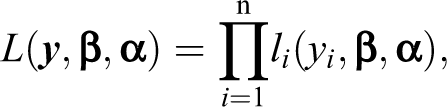
In the following, let us assume that we have
with
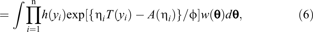
The GLMM is therefore a very general statistical analysis model. However, by properly specifying the conditional density

that can be used to perform, for example, not only linear regression analyses, analyses of variance, and analyses of covariance with or without (if

Here,
In general, the GLMM can accommodate multilevel-structured data sets through proper specification of
In terms of the GLMM, this model can be expressed as
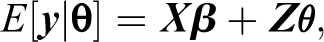
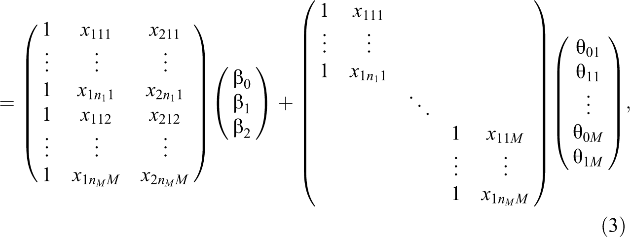
where
rather than to predict
Although a closed-form solution for estimating
Inference About the Fixed and Random Effects of the GLMM
Because our focus is on group comparisons, we are mainly interested in the question of whether these effects are equal across different populations. As mentioned above, the GLMM is a very general statistical analysis model. It incorporates, for example, the linear regression model or the analysis of variance model with random effects. Our aim in this section is to discuss a broad range of hypotheses tests (for both the single population case and the multiple population case) within the context of these specific models (Brame et al. 1998; Cai and Xia 2014; DeShon and Alexander 1994, 1996; Gujarati 1970a, 1970b; Moreno et al. 2005; Radhakrishnan and Robinson 1996; Skvarcius and Cromer 1971; Stroud 1974; Weerahandi 1987; Werts et al. 1976). We recognize, however, that a straightforward application of these specific tests to the estimators of the GLMM is not always possible. For example, as Ai and Norton (2003) have shown, the dummy variable approach, introduced by Gujarati (1970a, 1970b) and Skvarcius and Cromer (1971) within the context of the linear model for testing significant different slopes across groups, can produce biased inference when a probit or logit link is used. Consequently, instead of examining these specific tests, we discuss inference procedures directly relevant to the effects of the GLMM.
When discussing inference procedures for the fixed and random effects of the GLMM, we need, of course, to assume two different settings. In the first setting, that is, the single population case, the researcher has no interest in group differences (Stroup and Kachman 1994). In the second setting, that is, the multiple populations case, the researcher is interested in group differences. As mentioned above, different inference procedures exist for this setting. One possible way to test for these group differences is the dummy variable approach (Gujarati 1970a, 1970b; Skvarcius and Cromer 1971). This approach requires the researcher to combine the multiple data sets, use dummy variables to differentiate between these groups, and apply the GLMM to this combined data set to test the significance levels of the different slopes (interaction effects) across the groups (Rabe-Hesketh and Skrondal 2012). Another possibility is to apply the same GLMM independently to multiple data sets (one for each group) and then to compare the group-specific estimators (or predictors) across groups (Lazar and Zerbe 2011; Liao 2004). As we previously noted, the first procedure sometimes fails to provide valid results within the context of the GLMM, and for this reason, we do not consider it further. Hence, when conducting group comparisons of the estimators (or predictors) of the GLMM, we consider the second procedure in more detail. That is, here and in the following, we assume, among other premises, that the same GLMM is applied independently to multiple data sets proposed for the second setting. However, because inference procedures developed for the single population case usually provide a foundation for the more general case of multiple populations, we briefly consider these tests as well.
Single Population
For the single population case, inference about the fixed and random effects of the GLMM is usually based on the likelihood ratio test (LRT; McCulloch et al. 2008), the score test (Commenges and Jacqmin-Gadda 1997; Commenges, Letenneur, et al. 1994; Commenges, Olson, and Wijsman 1994; Lin 1997), or the Wald statistic (Stroup and Kachman 1994). When introducing the LRT, we can assume that the vector
with the likelihood given by
and where
Under certain regularity conditions (e.g., the true values of
The Wald statistic for inference about the fixed and random effects of the GLMM is based on the general linear hypotheses (Hsu 1991; Milliken and Graybill 1970; Olson 1975). As Stroup and Kachman (1994) and McCulloch et al. (2008) have pointed out, anyone using this test must assume that estimable functions

where
Several researchers have proposed the score test within the context of the GLMM to test the variance components given in
A comparison of the LRT and the Wald test makes clear that both tests are asymptotically equivalent under the null hypotheses
Irrespective of the power of the tests, we could argue that the LRT and the score test are generally superior to the Wald test because the confidence region based on these tests is exactly invariant under reparameterizations (Cox 1988). That said, using the Wald statistic does have utility because, unlike the LRT, researchers have to calculate the likelihood once only. The Wald test is therefore useful when a study requires the researcher to fit many models and to test a null hypothesis for every model. In general, then, consideration of both tests seems useful for drawing inferences from the parameters of the GLMM.
Multiple Populations
Here and in the following, assume that we have independently sampled
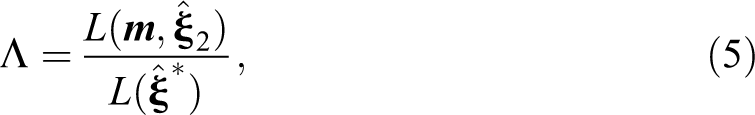
The likelihood for the hypothesis
Lazar and Zerbe (2011) recommend use of the following F-statistic for testing the null hypothesis
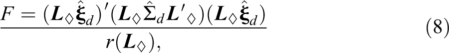
where
Another approach that avoids calculating LR
is the test statistic introduced by Liao (2004). Here, if we have the

with degrees of freedom equal to b (
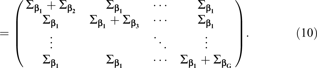
It is clear from equation (10) that Liao’s (2004) test can only be applied to multiple independent populations because otherwise the covariance parameters representing the different populations would have to be included in this covariance matrix. Although Liao (2004) presented examples of applications of this statistic, he did not provide a theoretical derivation for WL
, nor did he provide information about the power of WL
. In addition, the statistic in its current form is available only for the fixed effects of the GLM, and there might be situations where testing the random effects in the GLMM is also desirable. For example, in longitudinal studies of organizations, organizational trends are of interest (Hochweber and Hartig 2017). In this instance, a random sample of organizations (e.g., schools) is usually selected and then (clusters) samples of individuals (e.g., students) within these organizations are assessed at different time points (Feldman and McKinlay 1994). In cross-sectional designs, the samples are selected independently within each cluster at each time point (Feldman and McKinlay 1994:62), which means that the samples of individuals across clusters and time points can be considered as multiple independent populations, given the organizations. A common statistical approach for analyzing the resulting data (e.g., student’s test scores) is the random intercept model, a special case of the GLMM, as shown above. In this context, the random intercept effects can be considered as the cluster-specific means of the organizations. Thus, when the model is applied independently to each time point data set,
Our extended version of WL
, which includes the random effects, is applicable within the context of the GLMM, and allows testing of hypotheses of the form

with empirical covariance matrix
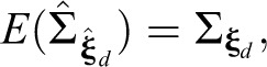
Like Liao’s (2004) statistic, this test can also only be applied to multiple independent populations. For a derivation of this statistic, see Online Appendix A (which can be found at https://journals.sagepub.com/doi/suppl/10.1177/0049124120986182). When
Thus, the WL
statistic is, in reality, a special case of WG
, and it is obvious that for

where WB
is asymptotically centrally
Power Analyses
Design of the Power Study
During our power analyses, we examined two link functions and two conditional distributions
In total, we assumed three fixed effects (one intercept and two slope parameters) and two random effects (one random intercept effect due to Level 3 and one random intercept effect due to Level 2). Thus:

where the order of
The power of the test WG can be expressed as

where
Noncentrality Parameter for
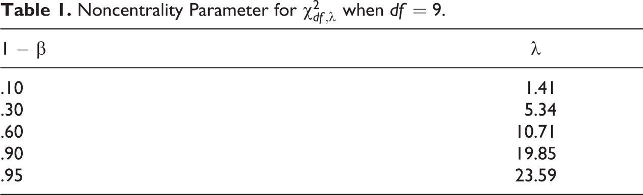
Because our hypotheses related only to the fixed effects, we chose random effects so that
Values for
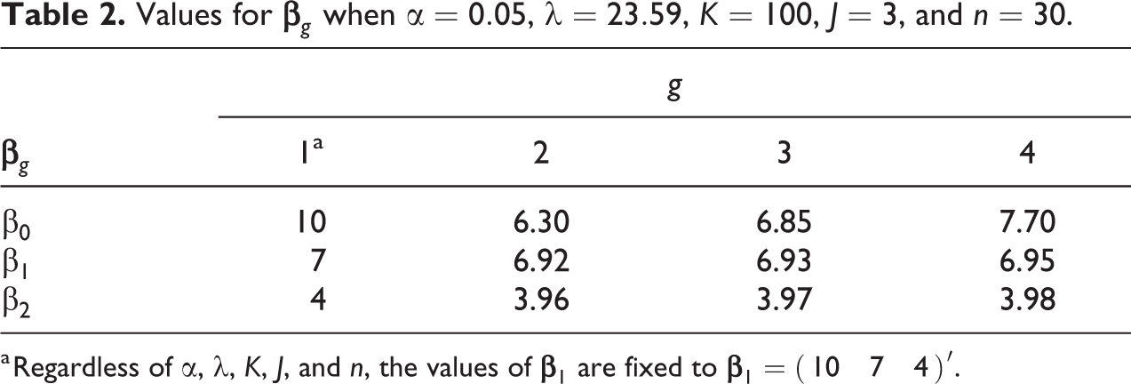
a Regardless of
For given values of sample sizes (i.e., values of K, J, and n),
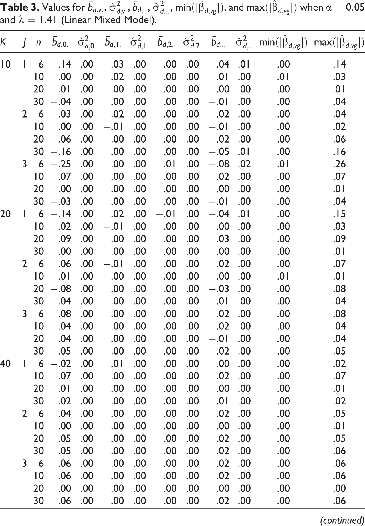
Evaluation Criteria
To evaluate our implemented simulation design, we examined different difference measures. These measures basically compare the difference between the given values (i.e., the input values) for the fixed effects, the random components, and (in the case of the LMM) the residual variance with the estimated values (i.e., the output values) of these quantities. For the fixed effects, we defined the matrix

and total variance
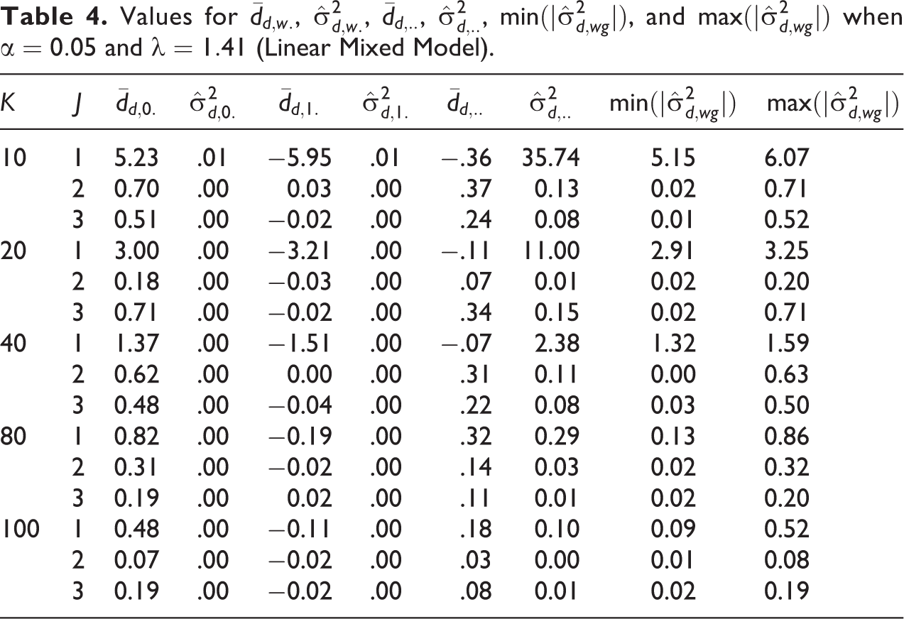
For the random components, we defined
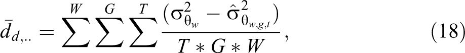
and the corresponding total variance
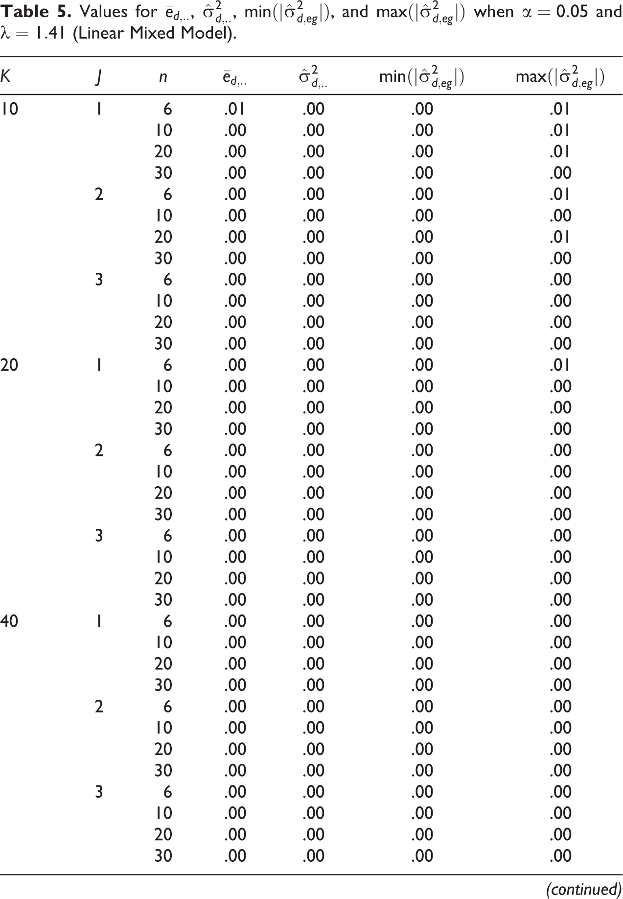
For the LMM, we also defined difference measures for the residual term. Given the simulated residual variance
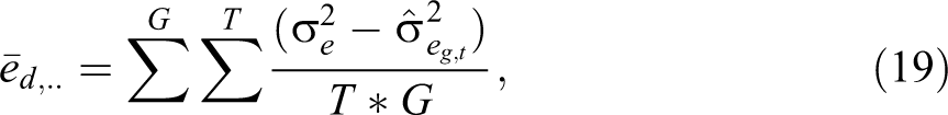
and the corresponding total variance
Results
Evaluation criteria
We obtained
For the fixed effects criteria
Values for
In regard to the evaluation criteria for the random components, we obtained
Values for
For the evaluation criteria of the residual variance, we obtained 300 values for the LMM. The average values of these criteria over these combinations for the LMM were
Values for
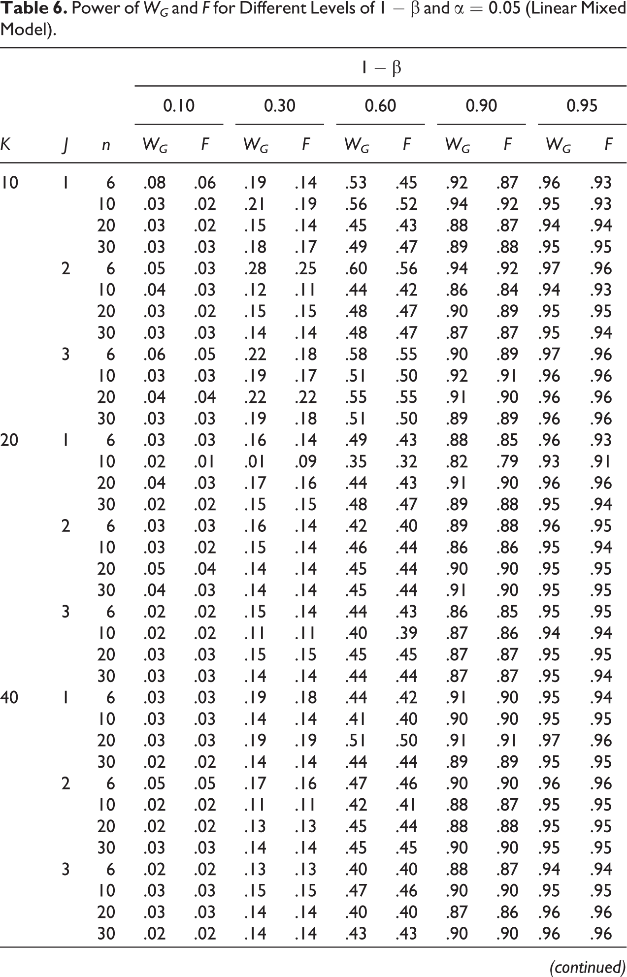
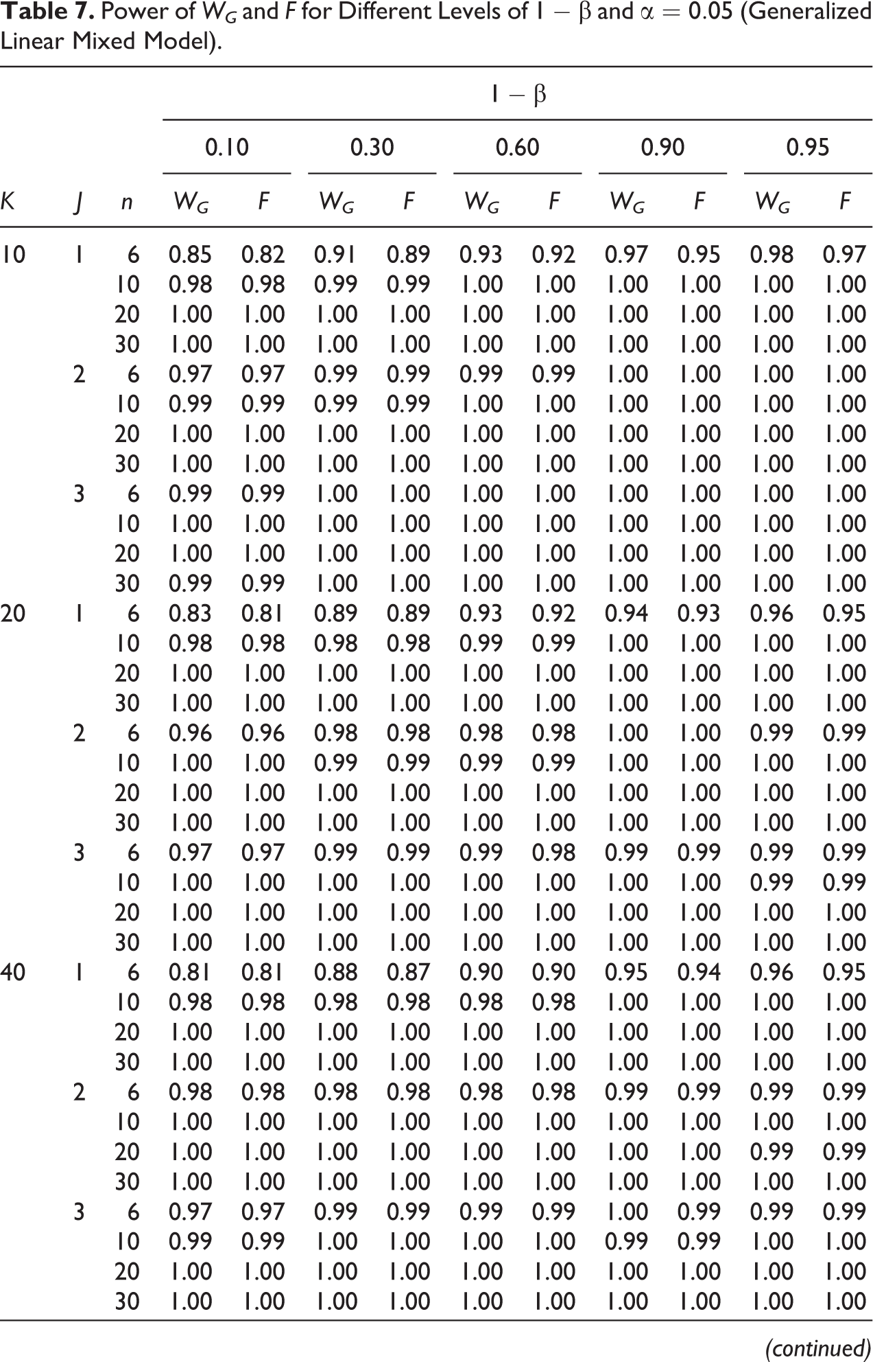
Power of WG and F
The average proportion of significant WG
values for the LMM across the 300 sample size combinations was
Power of WG
and F for Different Levels of
For the GLMM, the average proportions of significant WG
values and F across the 300 sample size combinations were
Power of WG
and F for Different Levels of
For a more objective view of the relationship between the observed power of WG
and F, the expected power, the model (LMM vs. GLMM), and the sample size, we estimated the parameters of a GLM (Nelder and Wedderburn 1972), where the number of significant WG
(F) values compared to the number of successful replications per combination was the dependent variable and the different levels of
Overall Measures of Fit for the Generalized Linear Model Analyses Where the Number of Significant Values for WG
and F per Successful Replication Is the Dependent Variable and the Test (WG
or F) as well as
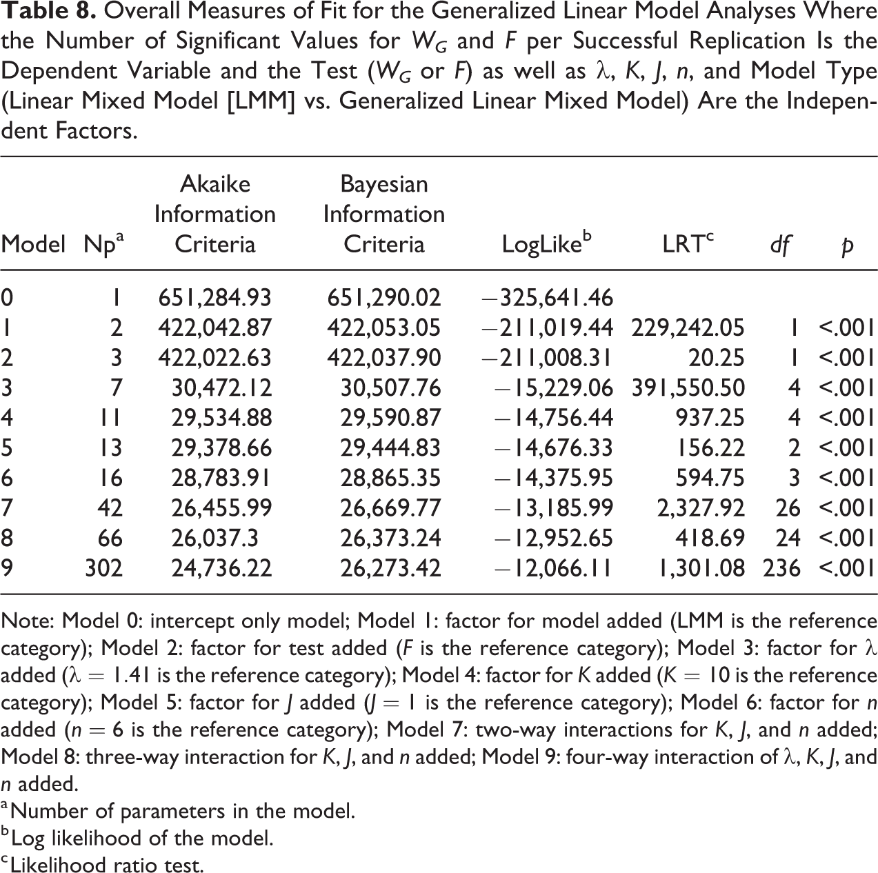
Note: Model 0: intercept only model; Model 1: factor for model added (LMM is the reference category); Model 2: factor for test added (F is the reference category); Model 3: factor for
a Number of parameters in the model.
b Log likelihood of the model.
c Likelihood ratio test.
As is evident from Table 8, all factors contributed significantly to the explanation of the power of WG
and F. Hence, the power of WG
and F depended strongly, as might be expected, on the effect size and not necessarily, as might also be expected, on the model.
7
The sample size as well as the test (WG
vs. F) also explained the power differences. As for sample size, the significant LRTs for Models 7 and 8 indicated that we needed to take into account the interaction effects between the sample sizes at the different levels and that the effect of sample size on power depended on the magnitude of
To obtain a closer look at the effects of the different factors associated with power, consider the estimated parameters for the different models in Table 9.
8
Note there that both statistics were more powerful for the GLMM model than for the LMM model, even when we took the different numbers of successful replications into account (Model 1;
Parameter Estimates for the Generalized Linear Model Analyses Where the Number of Significant Values for WG
and F per Successful Replication Is the Dependent Variable and the Test (WG
or F) as well as
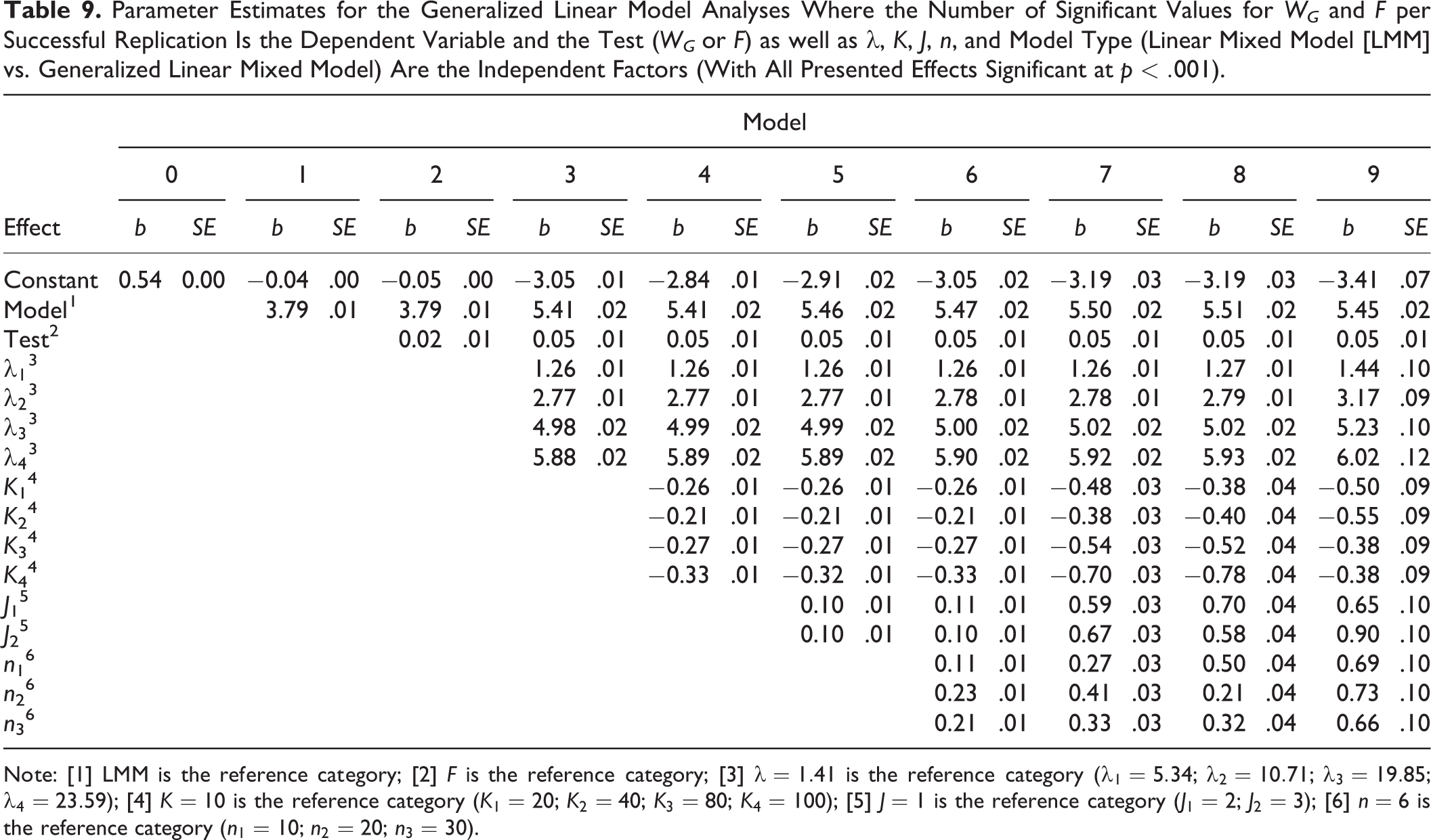
Note: [1] LMM is the reference category; [2] F is the reference category; [3]
Discussion
Our investigation of the power of the test statistics WG
and F via a simulation study saw us considering two special cases of the GLMM: a three-level hierarchical model with either a normally distributed dependent variable (LMM) and a Bernoulli distributed dependent variable (GLMM). In the simulation study, we varied the expected power and sample size for all three levels. Use of the expected power allowed us to calculate corresponding values for
Overall, we found that both statistics showed a negative bias when the expected power was small, that is, when the estimated power was smaller than the expected power. This finding implies that both tests have a higher probability of failing to reject the null hypothesis when it is in fact false (an increasing Type II error rate) for small effect sizes. During our simulation study, we found that we could not compensate for this behavior by increasing the sample size. Consequently, researchers expecting to find small effect sizes in studies comparing GLMM effects across multiple groups need to be more careful about accepting the null hypothesis. Further research is necessary to explore the magnitude of this negative bias when, for example, other GLMM models are used.
We also found that the WG statistic outperformed the F statistic with respect to estimated power. The fact that this advantage was small in magnitude may have practical relevance because the slight advantage that WG has over F implies that the negative WG bias is smaller than the F bias. As such, researchers may prefer to use WG instead of F, especially if they assume the effect sizes will be small. However, we also found that both tests had a higher estimated power when applied within the context of the GLMM model than within the context of the LMM model. Results not presented here (but which are part of this article’s Supplemental Material, which can be found at https://journals.sagepub.com/doi/suppl/10.1177/0049124120986182) showed the effect to be a general one because of the lack of a significant interaction between model type and test statistic.
In general, though, it seems that increasing the sample size at Level 1 or Level 2 increases the estimated power of WG and F. However, and somewhat unexpectedly, we found sample size at Level 3 had an inverse relationship to the estimated power, with both statistics appearing to be more powerful when the Level 3 sample size was relatively small. Thus, researchers using a three-level hierarchical model should, from the power perspective, think about increasing the Level 2 or Level 1 sample sizes but not necessarily the Level 3 size.
Example of Application
Introduction
In 2011, the IEA conducted the PIRLS and the TIMSS jointly for the first time. PIRLS has assessed the reading comprehension achievement of Grade 4 students every five years since 2001 (Mullis et al. 2012), while TIMSS has assessed the mathematics and science achievement of Grades 4 and 8 students every four years since 1995 (Martin et al. 2012). In 2011, 34 countries and three benchmark participants (hereafter, all 37 participants are referred to as countries) collected data on Grade 4 students’ educational achievement in three competence domains: reading comprehension, mathematics, and science (Martin and Mullis 2013).
Martin et al. (2013) performed a “school-effectiveness” analysis using the TIMSS/PIRLS 2011 combined data set. For their analysis, Martin and his colleagues used five school-effectiveness variables and two student home-background variables as predictors in country-specific HLMs. In other words, the authors applied the HLM independently to each country data set. One of the predictors is an index for home resources for learning (HRL), and in line with Bourdieu’s (1986) work on cultural capital, the HRL index can be interpreted as a measure of students’ socioeconomic and cultural home learning environments (Smith, Wendt, and Kasper 2017). Martin and colleagues used students’ achievement scores (reading comprehension, mathematics achievement, and science achievement) as dependent variables. Because the goal of the study was to “present an analytic framework that could provide an overview of how these relationships vary across countries” (Martin et al. 2013:110), it is reasonable to assume that the results from the hierarchical linear modeling would have been comparable across the participating countries.
One of Martin et al. (2013) major findings was that the strength of the relationships between the school-effectiveness variables and the student achievement scores decreased substantially in nearly all 37 countries when Martin et al. included home-background control variables in their models; country-specific effects were also apparent. For example, in 15 countries, only one of the five effectiveness indicators still presented a statistically significant prediction coefficient after Martin and his colleagues controlled for students’ home background. In four countries, three prediction coefficients remained significant. If the results of these analyses had, in fact, been comparable across the participating countries, then we could assume that in most of these countries, the strength of the relationships between school-effectiveness variables and student achievement would be relatively weak once Martin et al. controlled for student home background.
If we agree that the predictors used by Martin et al. (2013) can be interpreted as measures of students’ socioeconomic and cultural home learning environments, then we can view their results as being in line with current results in educational research. Within empirical educational research, operationalizing social background is often driven by interpretations of Bourdieu’s (1986) theory of capital, wherein economic capital is the most obvious form of power (Bourdieu 1986: 242-43). Bourdieu describes members of a society as foremostly arranged in hierarchical order, with, to put this in simplified terms, each hierarchical grouping having different volumes of certain capital resources (economic, cultural, social, and symbolic). With regard to human acting, thinking, and feeling, the forms of capital become embodied within habitus (Bourdieu 1998), a shared practical sense of social group membership. Gaining empirical access to the aforementioned practical sense or the identification of resources associated with capital forms is difficult, however.
It thus makes sense that the social-class models of students’ social background used in large-scale assessments like TIMSS and PIRLS endeavor to bring order to the complexity of social structure by simplifying and reducing the original theoretical complexity. This is the reason why single social background indicators have higher significance than other indicators. For example, considerable emphasis is placed on parents’ main occupation. The assumption here is that if we know the parents’ occupational level, we automatically know the family’s social position. Established standards in large-scale surveys like the Standard Index of Occupational Prestige Scores or the International Socio-Economic Index of Occupational Status have this kind of focus. Examples include the associated social prestige of occupations or the average income of occupational groups (Ganzeboom et al. 1992). According to the aforementioned theories, the items of the HRL scale, for example, can be classified as indicators of the economic and cultural capital of student’s families (Mullis et al. 2012).
The impact of student social background on achievement is one of the most consistently observed phenomena (see, e.g., Jehangir, Glas, and van den Berg 2015; Lavrijsen 2015; Martin and Mullis 2012; Martin et al. 2008; Mullis et al. 2007, 2008, 2012; Organization for Economic Cooperation and Development 2014; Pokropek, Borgonovi, and Jakubowski 2015; Sirin 2005). In a general sense, the observed achievement differences associated with student social background can be interpreted as educational inequalities (Walzebug and Kasper 2016). However, the relationship between the social background variables and the achievement scores varies considerably across participating countries in the study reported by Martin et al. (2013), suggesting different degrees of educational inequalities within the countries. However, it is not obvious, from the results that Martin et al. presented, which procedure they used for the cross-national comparisons of the fixed effects from the HLM. Among other concerns, we simply do not yet know whether the different degrees of educational inequality within the countries observed in the study can be considered statistically significant, which is why in the present example, we decided to reapply the country-specific HLMs.
However, because the effect of the school-effectiveness variables on achievement scores nearly vanished once social-background variables were included in the HLMs, and because we were mainly interested in the question of whether the different degrees of educational inequalities observed in Martin et al.’s (2013) study could be deemed statistically significant, we investigated only the relationship between the Grade 4 students’ mathematics achievement and the home-background control variables. Our analyses did not, therefore, include reading or science competencies and did not include school-effectiveness variables. We compared the fixed effects of this analysis cross nationally by applying the WB statistic we developed and which we have described in this article. Because we intended our analyses in this article to mainly demonstrate the application of the WB statistic, we discourage readers from interpreting the results with respect to any sophisticated theory or hypothesis.
Data and Variables
The data sets for TIMSS/PIRLS 2011 combined that we used for our study are freely available under the URL https://timss.bc.edu/timsspirls2011/international-database.html. The data sets contain the responses of 183,475 Grade 4 students across 37 countries. In addition to students’ achievement in mathematics, science, and reading, the data sets include students’ responses to questionnaire items designed to capture information on student-background variables as well as parents’ responses to items regarding parent-background variables. Of the freely available data sets, the country-specific data sets that we used have the name ASG***B1 and ASH***B1 appended to them, wherein *** stands for a country-specific code, ASG are the Grade 4 student-background data files, and ASH are the corresponding home-background data files.
9
The different data sets are also concatenated across the countries and then merged across the data resources. However, because analyzing a data set from 183,475 students from 37 countries was well beyond what we could include in this article, we restricted our analysis to data from the Grade 4 students from those countries that participated in TIMSS/PIRLS 2011 combined and were members of the European Union. This restriction resulted in a sample size of 15 countries (see Table 10) and a total sample size of
When constructing their home-background control model, Martin et al. (2013) used the variables ASBGHRL and ASBHAVG at the student level and ASBCHRL and ASBCAVG at the school level. ASBHAVG is the average of the variables ASBHELT and ASBHENT, and ASBCHRL and ASBCAVG form the school average of the variables ASBGHRL and ASBHAVG. The variables ASBGHRL, ASBHELT, and ASBHENT are contextual scales derived, via the partial credit model, from responses to specific sets of questions. A description of the contextual scales can be found in the context questionnaire scales section of Methods and Procedures in TIMSS and PIRLS 2011 (Martin and Mullis 2012). The variable ASBGHRL is an index for HRL, and it is based on several questionnaire items, including “number of books in the home” and “highest level of education of either parent.” ASBHELT is an index for early literacy tasks. It is based on an item that asked parents how often they or someone else did different activities in the home (e.g., read books, told stories) before the child began primary/elementary school. The index for early numeracy tasks, ASBHENT, is based on an item that asked parents to indicate which of a variety of numeracy-related activities (e.g., counting different things, playing with number toys) they or someone else did in the home before the child began primary/elementary school. The variables ASBGHRL, ASBHELT, and ASBHENT are part of the data sets that we used, while ASBHAVG, ASBCHRL, and ASBCAVG are the variables that we calculated. Table 10 includes descriptive statistics for these variables and for the mathematics achievement values. Because the means for ASBGHRL, ASBHAVG, ASBCHRL, and ASBCAVG in the table are highly similar to the values presented by Foy and O’Dwyer (2013), we assumed that, in general, we were using the same data as Martin et al. (2013) used in their analyses. 10
Descriptive Statistics for Mathematics Achievement and the Indicators of the Home-background Control Variables.
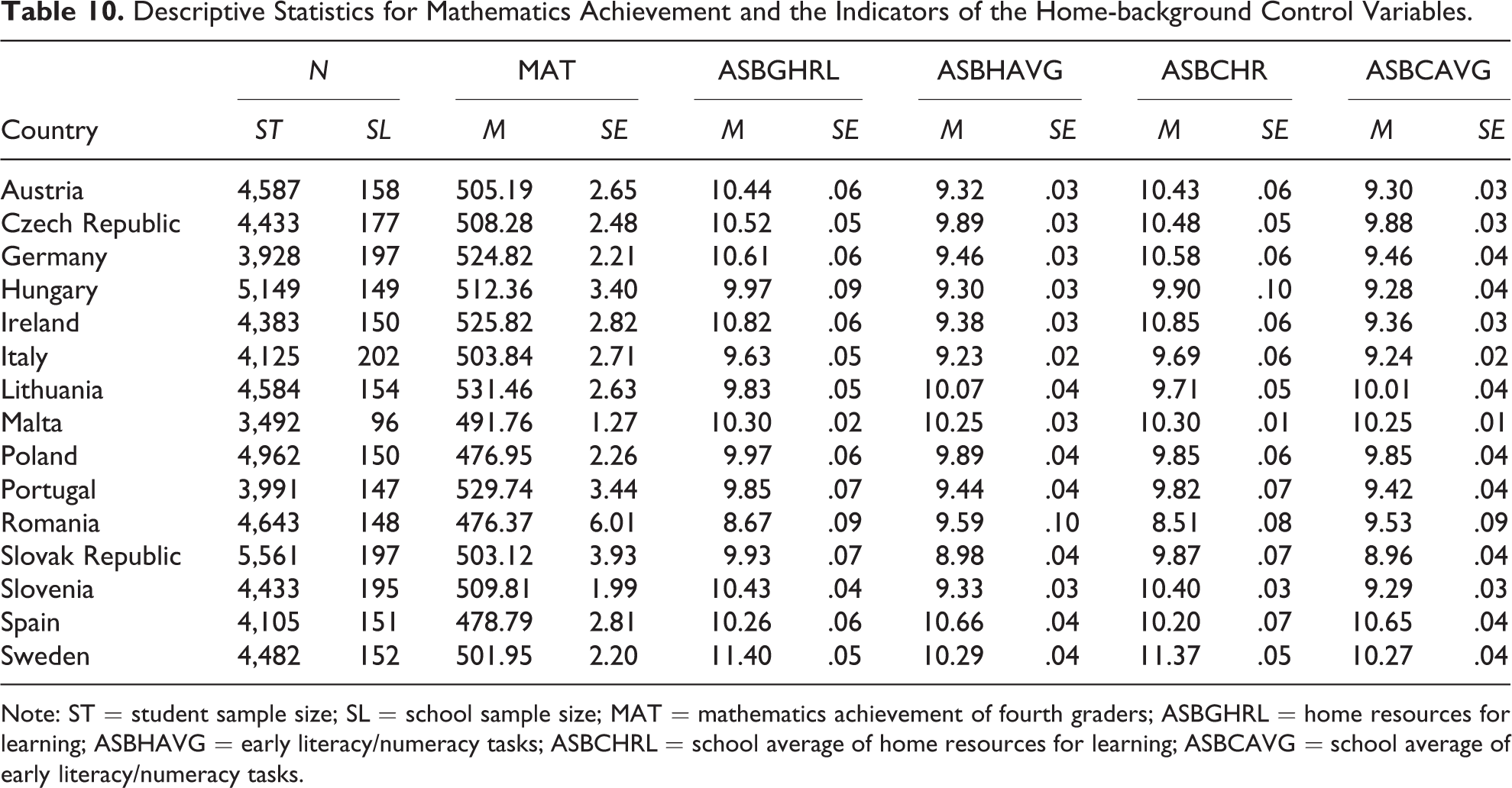
Note: ST = student sample size; SL = school sample size; MAT = mathematics achievement of fourth graders; ASBGHRL = home resources for learning; ASBHAVG = early literacy/numeracy tasks; ASBCHRL = school average of home resources for learning; ASBCAVG = school average of early literacy/numeracy tasks.
Prediction Model
The prediction model we used in our study was also very similar to the one Martin et al. (2013) used for their home-background control model. The variables in our country-specific HLM included ASBGHRL and ASBHAVG as the student-level predictors and ASBCHRL and ASBCAVG as the school-level predictors. We also included a random intercept term in our model, but unlike Martin et al. (2013), we did not include random effects for the slope coefficient of ASBGHRL and ASBHAVG. If, for example, for a given country g, we let

where the
Through a slight reformulation, the prediction model could also be expressed as a GLMM with an identity link function:
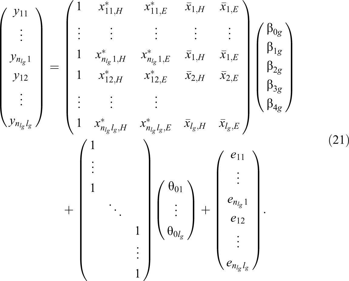
Here,
Weighting
The sampling procedure applied in TIMSS/PIRLS 2011 combined can be considered a stratified two-stage probability proportional to size systematic–clustered random sample. This procedure was applied separately in each participating country. In practice in most countries, it meant selecting a random sample of schools and then, within those schools, randomly selecting one class of Grade 4 students. Usually, all students within the selected classes participated in TIMSS/PIRLS 2011, which meant there was no need for a third sampling stage that would have involved sampling students within the classes. However, the sampling procedure meant the Grade 4 students in the participating schools did not have an equal chance of being selected. To compensate for this unequal selection probability, the TIMSS and PIRLS analysts weighted the data sets. The weights were basically the inverse of the selection probability, whether for the school, the class, or the student. One of these weights, TOTWGT, was normalized in a way that saw the sum of the weights across students within a country resulting in the population size. TIMSS and PIRLS typically use this weight for presenting results at the student level (Martin et al. 2012; Mullis et al. 2012). The descriptive statistics for mathematics achievement, ASBGHRL and ASBHAVG, presented in Table 10 were thus based on TOTWGT, and a Level 2 weight was used for ASBCHRL and ASBCAVG (accounts of the construction of level-specific weights in TIMSS and PIRLS can be found in Kasper, Schulz-Heidorf, and Schwippert 2018; Rutkowski et al. 2010). We also used level-specific weights in our GLMM analyses because various authors have suggested that these weights should be used for HLM models (Asparouhov 2006; Pfeffermann et al. 1998; Rabe-Hesketh and Skrondal 2006; Rutkowski et al. 2010). 12
Outcome
The outcome we designated for observation was the estimated
Missing Values and Software
Martin et al. (2013) used single imputation methods to impute the missing values in the HLMs predictor variables. However, they neither reported the details of their implemented imputation strategy nor provided readers with the imputed data set. Despite these omissions, we decided to approximate Martin et al. (2013) results as closely as possible by performing a single imputation for the missing values in the predictor variables. The method we used to do this was the Markov chain Monte Carlo method (Schafer 1997), in which all predictors and plausible values serve as the conditional variables. All of our analyses in this section are based on this imputed data set.
The software packages we employed for our analyses were SAS/STAT® and SAS/IML®, Version 9.4 (TS1M1) of the SAS System for Windows 13 (SAS Institute Inc. 2015a, 2015b), and we used the PROC GLIMMIX procedure to complete our GLMM analysis. We used PROC IML to implement the derived test statistics for the outcomes. Those readers wanting to form a full reconstruction of our analyses need to refer to the syntax and data sets that we used. These can be found in the material that supplements this article (which can be found at https://journals.sagepub.com/doi/suppl/10.1177/0049124120986182).
Results
Table 11 displays the fixed-effect vectors for the 15 TIMSS/PIRLS countries. Here, we can see that the fixed-effects coefficients and the corresponding standard errors for the Level 1 variables ASBGHRL and ASBHAVG are very similar to the results that Martin et al. (2013) found for their home-background control model. The small deviations evident in the table for these Level 1 effects can be attributed to differences between Martin and colleagues’ (2013) model and the imputation model we used. However, the fixed effects for the Level 2 variables ASBCHRL and ASBCAVG as well as the intercept vary considerably from Martin and colleagues’ results. This variance is expected because we introduced level-specific weights in our analysis while Martin et al. (2013) used a combined weight. As Rabe-Hesketh and Skrondal (2006) showed, level-specific weights affect estimation of the random components and in turn estimation of the corresponding fixed-effect terms. As Martin et al. (2013) also found out, the fixed-effect vectors vary considerably across countries. Thus, although every country shows a relationship between students’ social background and students’ observed mathematics achievement values, the nature and strength of this relationship depend on the country in which the students were being taught. In Portugal, for example, the effect sizes are considerably lower than those in Slovenia, while in Slovenia, the effect of student-level home resources on mathematics achievement seems to be much greater than in the remaining countries.
Estimated Fixed Effect Vectors of the Applied Generalized Linear Mixed Model.
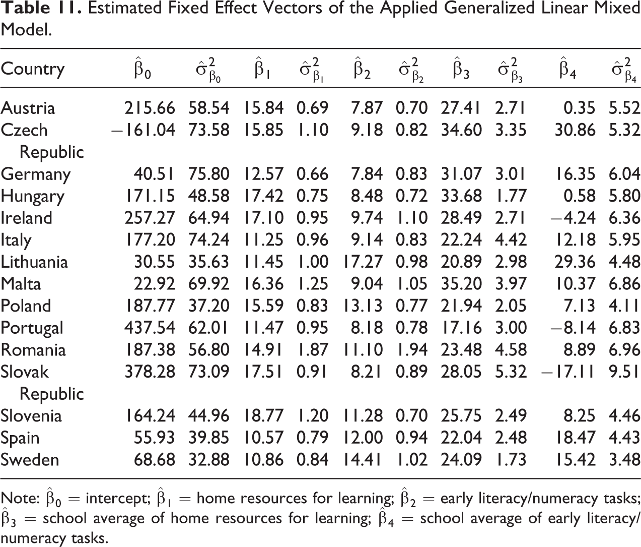
Note:
To determine whether the observed differences in the fixed-effect vectors across countries were statistically significant, we calculated WB
with reference to the hypothesis
Pairwise Comparison Between Country’s Fixed Effects Vectors From the Generalized Linear Mixed Model (WB Values Above the Diagonal and p Values Below the Diagonal).
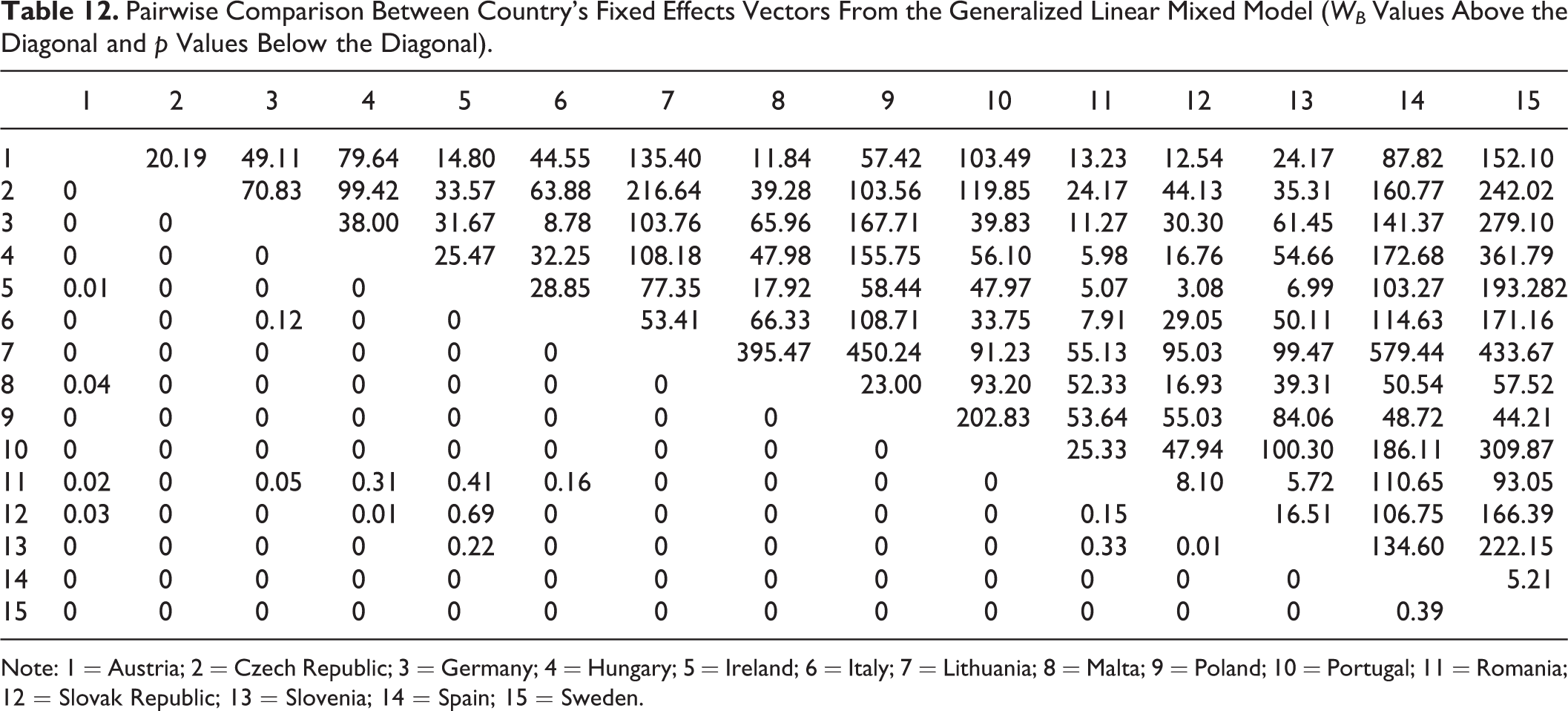
Note: 1 = Austria; 2 = Czech Republic; 3 = Germany; 4 = Hungary; 5 = Ireland; 6 = Italy; 7 = Lithuania; 8 = Malta; 9 = Poland; 10 = Portugal; 11 = Romania; 12 = Slovak Republic; 13 = Slovenia; 14 = Spain; 15 = Sweden.
As is evident from the table, most of the pairwise comparisons resulted in highly statistically significant different fixed-effect vectors across countries. However, in 16 cases, the p value is greater than or equal to
Discussion
After Martin et al. (2013) performed their “school-effectiveness” analysis using the TIMSS/PIRLS 2011 combined data set, they compared the results of their analyses of the data across the participating countries. During this process, they referred to the fixed-effects vectors
In line with Bourdieu’s (1986) work on cultural capital, TIMSS and PIRLS derive variables for the home-background control model (ASBGHRL and ASBHAVG) to serve as indicators for students’ social background. In general, like Martin et al. (2013), we have shown, for every country considered here, a strong association between these indicators and mathematics achievement. Hence, we must assume strong educational inequalities in all these countries. These inequalities are present not only at the student level, that is, students with small values on the social background indicators show lower performance in mathematics than students with higher values on these indicators, but also at the class level, meaning that classes with lower average values on the social background indicators show lower performance on the average mathematics achievement score (where the average is taken over the students within a class). Also, like Martin et al. (2013), we have shown that countries can be grouped according to the strength of these educational inequalities. Furthermore, whereas the overall WB statistics were highly statistically significant, the WB statistics for the pairwise comparisons were not always statistically significant. Thus, having taken the results of our study into account, we can conclude that the degree of educational inequality not only varies considerably across the countries considered here but also is of a similar size in several other countries.
Although our results indicate that the grouping made by Martin et al. (2013) needs closer consideration, we do caution that our example study has some limitations. First, because we did not know which procedure Martin et al. (2013) used to compare the fixed effects from their HLMs analyses, we were not able to assess the reliability of this approach and especially so with respect to the procedure we used. Second, although Martin et al. (2013) based their comparisons on the full HLMs model, that is, the model that included not only the home-background control variables but also the school-effectiveness variables, our models included only the home-background control variables. We consider that including additional variables in our models would not alter the basic results of the dissimilarity of the fixed-effects vectors
General Discussion and Conclusions
Basing our work on the Wald statistic, we developed an asymptotic test statistic for across-group comparisons of the fixed and random effects from the GLMM. The test can be used when the GLMM is applied independently to each group’s data set, assuming we have the same conditional distributional family of the dependent variable, link function, and distributional family for the random effects across groups. We also need to assume that the fixed effects are independent from the random effects and that both effects are asymptotically normally distributed. Under these conditions, our statistic can be used to test hypotheses of the form
Although the assumptions under which we developed our test statistic are very common within the context of the GLMM, it might be desirable to have a test statistic that is also valid under more general assumptions (e.g., not normally distributed random effects). Also, because it is usually not the random effects themselves but the variance components that are of interest, a valid test that simultaneously tests the fixed effects and the variance components in the setting considered here is desirable. However, development of such a test needs to take into account the findings from Verbeke and Molenberghs (2000, 2003) that emphasized the need to address the problem of invalid tests when the parameters are on the boundary of the parameter space. Finally, because our theoretical derivations of the test are very general, and we can thus assume that the test is applicable to a broad range of GLMM subtypes, investigating the applicability of this test to several special versions of this model (e.g., the HLM with cross-level interactions) in more detail is worthwhile.
By using power studies, we showed that when a hierarchical data structure is assumed, our test statistic WG outperformed, in terms of estimated power, the F test statistic proposed by Lazar and Zerbe (2011). We also showed that both tests had a negative bias (i.e., that of underestimating the expected power) when the expected power was small. Thus, although the extent to which the WG statistic outperformed the F test was relatively small, it can still be relevant because in situations where we expect the power to be relatively small, the negative bias for WG is smaller. We furthermore showed that increasing the sample size at Level 1 and at Level 2 had a positive effect on the estimated power of both statistics and that sample size at Level 3 was negatively related to the estimated power. Hence, in regard to power, we consider increasing sample sizes at both Levels 1 and 2 is reasonable but that the same cannot necessarily be said in relation to Level 3.
We found the power studies very helpful for gaining an impression of how WG and F perform within the context of the GLMM. However, because the GLMM is a very general model, and because it was beyond the scope of this article to look at all possible specific formulations of it, we had to restrict our power studies to a concrete formulation of the GLMM. We accordingly assumed a hierarchical data structure and two kinds of conditional distributions for the dependent variable with a corresponding link function. Although hierarchical data structures are very common in, for example, educational psychology, power studies featuring different formulations of the GLMM should provide further information about the performance behavior of WG . The negative relationship between sample size at Level 3 and the estimated power of WG and F also merits further consideration.
We also provide a practical example for the application of the WG statistic. Here, we reanalyzed part of the TIMSS/PIRLS 2011 combined data sets that Martin et al. (2013) used for their “school-effectiveness” analysis. During their analysis, Martin and his colleagues used five school-effectiveness variables and two student home-background variables as predictors in country-specific HLMs. In general, once the home-background variables had been controlled for, the school-effectiveness variables no longer showed associations with students’ achievement, which is why we confined our reanalysis to the home-background control variables only. In line with Bourdieu’s (1986) work on cultural capital, home-background control variables can be interpreted as a measure of students’ socioeconomic and cultural home learning environments. In a general sense, we can consider associations between these variables and students achievement as educational inequalities (Walzebug and Kasper 2016). Therefore, the associations between these variables and students’ achievement found in Martin et al.’s study shows us the existence of educational inequalities in all of the participating countries.
However, the relationships between the social background variables and the achievement scores varied considerably across the participating countries in Martin et al.’s (2013) study, suggesting different degrees of educational inequality within the countries. Unfortunately, it is not clear from the results that Martin and his colleagues presented which procedure they used for the cross-national comparisons of these effects. Accordingly, we do not know whether the different degrees of educational inequality within the countries can be considered as statistically significant. It was for this reason that we decided to reapply the country-specific HLMs, using only the social background variables. We then compared the fixed effects of this analysis cross nationally by applying the test statistic we developed. Our results suggest that, in general, we can consider the observed educational inequalities as statistically significant. Moreover, because not all of the pairwise comparisons of the fixed effects across countries were statistically significant, we can assume that educational inequalities exist in all participating countries and that the extent of these inequalities is of similar size in some countries. This finding provides educational researchers with the opportunity to compare countries with a lesser degree of educational inequality, such as Portugal, with countries with a higher degree of educational inequality, such as Slovenia.
Also, while we provided a practical example for the application of the WG statistic in this article, we do caution that our example-related work has some limitations. First, we examined only one achievement domain (mathematics achievement) out of three domains (reading achievement, science achievement, and mathematics achievement). Consequently, it is not clear whether our results will also emerge as valid if we consider other educational outcomes. Second, as Walzebug and Kasper (2016) discuss, the indicators used in our study measured the social background of the students only and in a very simplified manner. Although these measures are typically not measurement invariant across countries (Wendt et al. 2017), Martin et al. (2013) assumed that they are measurement invariant, as did we during our reanalysis. The assumption of measurement invariant is a necessary requirement for validity across group comparisons. It therefore remains unclear as to what results might be observed if the indicators used for social background were proven to be measurement invariant. A third limitation of our reanalysis is the sample size. Whereas Martin et al. (2013) analyzed the data sets from 37 countries, the only data sets we analyzed were those from the 15 countries that were the members of the European Union in 2011. Hence, our results apply only to these 15 countries. With regard to international comparative educational research studies, it therefore seems worthwhile for us to expand our analyses to include all countries that participated in TIMSS and PIRLS.
Supplemental Material
Supplemental Material, sj-pdf-1-smr-10.1177_0049124120986182 - Multiple Group Comparisons of the Fixed and Random Effects From the Generalized Linear Mixed Model
Supplemental Material, sj-pdf-1-smr-10.1177_0049124120986182 for Multiple Group Comparisons of the Fixed and Random Effects From the Generalized Linear Mixed Model by Daniel Kasper, Katrin Schulz-Heidorf and Knut Schwippert in Sociological Methods & Research
Supplemental Material
Supplemental Material, sj-pdf-2-smr-10.1177_0049124120986182 - Multiple Group Comparisons of the Fixed and Random Effects From the Generalized Linear Mixed Model
Supplemental Material, sj-pdf-2-smr-10.1177_0049124120986182 for Multiple Group Comparisons of the Fixed and Random Effects From the Generalized Linear Mixed Model by Daniel Kasper, Katrin Schulz-Heidorf and Knut Schwippert in Sociological Methods & Research
Supplemental Material
Supplemental Material, sj-zip-1-smr-10.1177_0049124120986182 - Multiple Group Comparisons of the Fixed and Random Effects From the Generalized Linear Mixed Model
Supplemental Material, sj-zip-1-smr-10.1177_0049124120986182 for Multiple Group Comparisons of the Fixed and Random Effects From the Generalized Linear Mixed Model by Daniel Kasper, Katrin Schulz-Heidorf and Knut Schwippert in Sociological Methods & Research
Supplemental Material
Supplemental Material, sj-zip-2-smr-10.1177_0049124120986182 - Multiple Group Comparisons of the Fixed and Random Effects From the Generalized Linear Mixed Model
Supplemental Material, sj-zip-2-smr-10.1177_0049124120986182 for Multiple Group Comparisons of the Fixed and Random Effects From the Generalized Linear Mixed Model by Daniel Kasper, Katrin Schulz-Heidorf and Knut Schwippert in Sociological Methods & Research
Supplemental Material
Supplemental Material, sj-tex-1-smr-10.1177_0049124120986182 - Multiple Group Comparisons of the Fixed and Random Effects From the Generalized Linear Mixed Model
Supplemental Material, sj-tex-1-smr-10.1177_0049124120986182 for Multiple Group Comparisons of the Fixed and Random Effects From the Generalized Linear Mixed Model by Daniel Kasper, Katrin Schulz-Heidorf and Knut Schwippert in Sociological Methods & Research
Supplemental Material
Supplemental Material, sj-tex-2-smr-10.1177_0049124120986182 - Multiple Group Comparisons of the Fixed and Random Effects From the Generalized Linear Mixed Model
Supplemental Material, sj-tex-2-smr-10.1177_0049124120986182 for Multiple Group Comparisons of the Fixed and Random Effects From the Generalized Linear Mixed Model by Daniel Kasper, Katrin Schulz-Heidorf and Knut Schwippert in Sociological Methods & Research
Footnotes
Authors’ Note
All authors made substantial contributions to the conception, the design, and the interpretation of the results of the study, D.K. and K.S. read and approved the manuscript. In addition, D.K. conducted the analysis and was responsible for the statistical explanations. D.K. and K.S.H. drafted the manuscript. In this article, data sets from the International Association for the Evaluation of Educational Achievement (IEA) study Trends in International Mathematics and Science Study (TIMSS) 2011 are analyzed. These data sets and a corresponding documentation of the data sets are freely available under the URL (![]() ).
).
Acknowledgments
The authors acknowledge the anonymous reviewers for the attention and expertise they generously shared to support the production of this article. We further thank Paula Wagemaker for pre-submission English editing support.
Declaration of Conflicting Interests
The author(s) declared no potential conflicts of interest with respect to the research, authorship, and/or publication of this article.
Funding
The author(s) received no financial support for the research, authorship, and/or publication of this article.
Supplemental Material
Supplemental material for this article is available online.
Notes
References
Supplementary Material
Please find the following supplemental material available below.
For Open Access articles published under a Creative Commons License, all supplemental material carries the same license as the article it is associated with.
For non-Open Access articles published, all supplemental material carries a non-exclusive license, and permission requests for re-use of supplemental material or any part of supplemental material shall be sent directly to the copyright owner as specified in the copyright notice associated with the article.