Sage Journals: Discover world-class research

Abstract

Small area estimation (SAE) plays a crucial role in the social sciences due to the growing need for reliable and accurate estimates for small domains. In the study of well-being, for example, policy makers need detailed information about the geographical distribution of a range of social indicators. We investigate data dimensionality reduction using factor analysis models and implement SAE on the factor scores under the empirical best linear unbiased prediction approach. We contrast this approach with the standard approach of providing a dashboard of indicators or a weighted average of indicators at the local level. We demonstrate the approach in a simulation study and a real data application based on the European Union Statistics for Income and Living Conditions for the municipalities of Tuscany.

Keywords

composite estimation direct estimation EBLUP factor analysis factor scores model-based estimation

Introduction

Measuring poverty and well-being is a key issue for policy makers requiring a detailed understanding of the geographical distribution of social indicators. This understanding is essential for the formulation of targeted policies that address the needs of people in specific geographical locations. Most large-scale social surveys can only provide reliable estimates at a national level. A relevant survey for analyzing well-being in the European Union (EU) is the European Union Statistics for Income and Living Conditions (EU-SILC). However, these data can only be used to produce reliable direct estimates at the Nomenclature of Territorial Units for Statistics (NUTS) 2 level (Giusti, Masserini, and Pratesi 2015) which are generally large regions within a country. For example, in Italy one such NUTS 2 region is Tuscany. Hence, if the goal is to measure poverty and well-being indicators at a subregional level, such as NUTS 3 or Local Administrative Units (LAU) 2 which correspond to the Italian municipalities, the indicators may not be directly estimated from EU-SILC. In fact, the domains corresponding to the regions under NUTS 2 are so-called unplanned domains where domain membership is not incorporated in the sampling design, and therefore, the sample size in each domain is random (and may be large or small) and in many cases zero. In this case, indirect model-based estimation methods, in particular small area estimation (SAE) approaches, can be used to predict target parameters for the small domains.

SAE is defined as a set of statistical procedures with the goal of producing efficient and precise estimates for small areas as well as for domains with zero sample size (Rao and Molina 2015). An area is defined as small, if the area is an unplanned domain and the specific sample size may not be large enough to provide reliable direct design-based estimates. Small areas can also be defined by the cross-classification of geographical areas by social, economic, or demographic characteristics.

SAE methods can be classified into two approaches: the unit-level and the area-level approach. The unit-level approach is used when covariates are available for each unit of the population, for example, from census or administrative data, while the area-level approach is used when covariate information is known only at the area level. The use of the error-components model by Battese, Harter, and Fuller (BHF; 1988), also known as the BHF model, is commonly used for the unit-level SAE approach. In the SAE literature, estimation methods include empirical best linear unbiased prediction (EBLUP), empirical Bayes (EB), and hierarchical Bayes (HB). The EBLUP method can be used under linear mixed models, while the EB and HB methods can be used under generalized linear mixed models. For a review of these methodologies and their extensions, we refer to Rao and Molina (2015).

A second important issue we consider in this article is the multidimensionality of well-being indicators. Although it is generally agreed that well-being is a multidimensional phenomenon (Organization for Economic Cooperation and Development [OECD] 2013), there is continuing debate about the suitability of combining social indicators based on taking their average or using a dashboard of single indicators. On the one hand, Ravallion (2011) argues that a single multidimensional composite indicator in the context of poverty measurement leads to a loss of information, and on the other hand, Yalonetzky (2012) points out that composite indicators are necessary when the aim is to measure multiple deprivations within the same unit (individual or household). For a theoretical review of statistical properties of multidimensional indicators obtained by multivariate statistical techniques and related problems, we refer to Krishnakumar and Nagar (2008) and Bartholomew et al. (2008).

Taking this latter view, an approach to reducing data dimensionality is to consider the multidimensional phenomena as a latent variable construct measurable by a set of observed variables and estimated using a factor analysis model. Factor scores are estimated from a factor analysis model and are defined as a composite variable computed from more than one response variable. Indeed, factor scores provide details on each unit’s placement on the factor. When we have a substantive framework where a set of variables explains a latent construct, the confirmatory factor analysis (CFA) modeling approach can be used. In the context of well-being measurement, a framework of indicators is generally provided a priori by official statistics or international organizations and thus are treated as fixed. The vector of unobserved variables represents a set of variables that jointly describe the underlying phenomenon. We note other work on the use of factor analysis modeling in latent well-being measurement to reduce data dimensionality in Ferro Luzzi, Fluckiger, and Weber (2008) and Gasparini et al. (2011). There are also other approaches which reduce dimensionality of measurement frameworks such as the Fuzzy set approach in Lemmi and Cheli (2006). Betti, Gagliardi, and Verma (2017) and Betti and Gagliardi (2017) discuss the variance estimation problem of multidimensional measures of poverty and deprivation obtained via the Fuzzy set approach using the jackknife method.

Once factor scores are estimated from the factor analysis model, they can be used to conduct further statistical analysis. For instance, they can be used as dependent or independent variables of a regression or predictive analyses to answer particular research questions. Kawashima and Shiomi (2007) use factor scores in order to conduct an analysis of variance on high school students’ attitudes toward critical thinking and tested differences by grade level and gender. In addition, Bell, McCallum, and Cox (2003) investigated reading and writing skills where they extracted the factors and estimated factor scores before using them in a multiple regression analysis model. Skrondal and Laake (2001) note that using factor scores as dependent variables in regression modeling produces consistent estimates of model parameters since any measurement error from the factor analysis model is absorbed into the prediction error and coefficients are not attenuated (see also Fuller and Harter 1987). Also, as highlighted in Kaplan (2009), we can assume that the specific variances from the factor analysis model are very small compared to the prediction error.

In the current literature on SAE of social indicators, there is a research gap on the estimation of multidimensional indicators. In particular, the use of factor scores and factor analysis in SAE models is an open area of research. This research area is important when we have to deal with data dimensionality in the estimation of social indicators at a local level. In this article, we consider economic well-being as a latent variable construct with the aim of reducing the dimensionality of well-being indicators. We then implement the unit-level SAE approach on the factor scores in both a simulation study and on real data from EU-SILC for the region of Tuscany, Italy.

In particular, we address the problem of providing reliable SAE of multidimensional economic well-being phenomena starting from an established well-being measurement framework, such as the Italian Equitable and Sustainable Well-being framework Benessere Equo e Sostenibile (BES). As mentioned, these frameworks are already developed within countries and are commonly used for the measurement of the sustainable development goals. Therefore, we follow a two-step procedure: first latent variables are estimated based on the measurement framework via a CFA model, and second the small area estimates along with their measures of uncertainty are computed via the EBLUP approach.

This article is organized as follows. In the second section, we describe the factor analysis model for reducing data dimensionality on a dashboard of economic well-being indicators. In the third section, we review the unit-level SAE approach according to the BHF model and present the point estimation of the EBLUP for small area means. In the fourth section, we show results of a simulation study considering factor scores for data dimensionality reduction and contrast our approach to the typical approach of averaging single univariate EBLUPs on the original variables. When averaging single univariate EBLUPS on the original variables, we consider both a simple average and a weighted average where the weights are defined by the factor loadings. Moreover, we develop a parametric bootstrap algorithm to estimate mean squared errors (MSEs) of the EBLUP of factor score means and evaluate its properties. In the fifth section, we discuss multidimensional economic well-being in Italy considering indicators from the Italian framework BES (Equitable and Sustainable Well-being) 2015 (ISTAT 2015). Also, using real data from EU-SILC 2009 for the area of Tuscany, we apply the proposed method and compute small area EBLUPs for factor score means and their MSE for each Tuscany municipality (LAU 2). Finally, in the sixth section, we conclude with some final remarks and a general discussion.

Using Factor Scores for Data Dimensionality Reduction

In this section, we provide a general discussion on the use of factor analysis models to reduce data dimensionality and focus on the estimation of factor scores. Since the focus of the application in Economic Well-being in Tuscany: A Multidimensional Approach section is on measuring economic well-being based on a given substantive framework and a small number of single indicators, we consider here a one-factor analysis model. We acknowledge that in the presence of more complex multidimensional phenomena, one factor may not explain the total variability. Moretti, Shlomo, and Sakshaug (2017) investigate the issue of multiple latent factors under a multivariate SAE approach.

Issues in Composite Indicators

Multivariate statistical methods aim to reduce the dimensionality of a multivariate random variable Y . Formally, consider a R^K space, where K denotes the number of observed variables where we want to represent the observations in a reduced space R^M with $M ≪ K$ . Bartholomew et al. (2008) suggests several multivariate statistical techniques in order to deal with data dimensionality reduction in the social sciences (e.g., principal component analysis, factor analysis models, multiple correspondence analysis). In this work, we consider the linear one-factor model, where the factor can be interpreted as a latent characteristic of the individuals revealed by the original variables. This model allows for making inference on the population, since the observable variables are linked to the unobservable factor by a probabilistic model to develop a composite indicator (Bartholomew et al. 2008).

There is an ongoing debate about how to construct indicators which are useful for decision makers to inform policies. Saisana and Tarantola (2002) and Nardo et al. (2005) emphasize that composite indicators are important when a summary of multidimensional phenomena is needed and propose factor analysis models. Nardo et al. (2005) highlight that factor analysis models reduce the data dimensionality of a set of subindicators while keeping the maximum proportion of the total variability of the observed data.

Given our focus on data dimensionality reduction from a well-established multidimensional well-being framework, the BES framework for Italy (ISTAT 2015), the single indicators have already been grouped into well-being dimensions. One such dimension is the economic well-being dimension. Therefore, we use factor analysis models under a confirmatory approach.

Factor scores are estimated from a CFA model. They are defined as composite estimates providing details on a unit’s placement on the latent factor (DiStefano, Zhu, and Mindrila 2009). The factor scores, once estimated, are easy to interpret: They have the same economic interpretation of the observed responses as they are strongly linearly related to these via a linear model.

There have been some first attempts in SAE and data dimensionality reduction using factor analysis (e.g., Smith et al. 2015). Here, the construction of the composite indicators was on the small area EBLUPs of the single indicators. In our approach, we first construct the composite indicator from the factor analysis model and then obtain small area estimates of the average factor score. We also focus on MSE estimation for the estimates.

The Linear One-factor Analysis Model

Let us consider a $K \times 1$ vector of observed variables Y and we assume that they are linearly dependent on a factor f . Thus, we can write the following linking model (Kaplan 2009):

Y = Λ f + ∊,

where $∊$ denotes a vector $K \times 1$ containing both measurement and specific error, and $Λ$ is a $K \times 1$ vector of factor loadings.

It is assumed that:

$E (∊) = 0$ ,

$Var (∊) = Θ$ ,

$∊ \sim N (0, Θ)$ ,

$∊$ ‘s components are uncorrelated,

$E (f) = 0$ ,

$Cov (∊, f) = 0$

Therefore, the covariance matrix of the observed data is given by:

Σ = Cov (Y Y') = Λ Φ Λ' + Θ,

where $Φ$ denotes the factor variance, and $Θ$ is a $K \times K$ diagonal matrix of specific variance.

The maximum-likelihood (ML) approach is used to estimate the model parameters. ML equations under factor analysis models are complicated to solve, so iterative numerical algorithms are proposed in the literature (see, e.g., Mardia, Kent, and Bibby 1979). The log-likelihood function $ℓ$ of the data Y can be written as follows (Härdle and Simar, 2012):

ℓ (Y; Λ, Θ) = - \frac{n K}{2} log (2 π) - \frac{n}{2} log | Σ | - \frac{n - 1}{2} t r (S Σ^{- 1}),

where S denotes the sample covariance matrix.

After the model parameters are estimated, the factor scores are also estimated. Factor scores are defined as estimates of the unobserved latent variables for each unit i. For a review of estimated factor scores, we refer to Johnson and Wichern (1998). Using Bartlett’s method, the individual factor scores estimate for i = 1,…, n are given by Bartholomew, Deary, and Lawn (2009):

{\hat{f}}_{i} = \hat{Γ} \hat{Λ}' {\hat{Θ}}^{- 1} y_{i},

where $\hat{Γ} = \hat{Λ}' {\hat{Θ}}^{- 1} \hat{Λ}$ and y _i denotes a K-dimensional vector of observations of K components of Y for $i = 1, \dots, n$ .

Bartlett’s method produces unbiased estimates of the true factor scores (Hershberger 2005).

In the application presented in Economic Well-being in Tuscany: A Multidimensional Approach section, we also have binary dependent variables. According to L. K. Muthén and Muthén (2012), logistic regression is employed for binary dependent variables where the following transformation is applied in a single-factor model for each observed variable k:

logit [π_{k} (f)] = log \frac{π_{k} (f)}{1 - π_{k} (f)} = λ_{k} f, k = 1, \dots, K .

where $π_{k} (f)$ denotes the probability that the dependent variable is equal to one, and $\frac{π_{k} (f)}{1 - π_{k} (f)}$ the odds. We can then write the following expression:

π_{k} (f) = \frac{exp (λ_{k} f)}{1 + exp (λ_{k} f)},

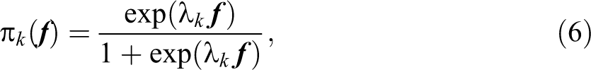
which is monotonic in f and with domain in the interval [0,1].

In the presence of binary and continuous observed variables and under a maximum likelihood estimation approach, the factor scores may be estimated via the expected posterior method described in Muthén (2012) and applied in Mplus, Version 7.4.

SAE Using EBLUP

A class of models for SAE is the mixed effects models where we include random area-specific effects in the models and take into account the between-area variation.

Notation

Let $d = 1, \dots, D$ denote small areas for which we want to compute estimates of the target population parameter for each d, in our case the population mean ${\bar{F}}_{d}$ of the factor score. For a sample $s \subset Ω$ of size n drawn from the target population of size N, the nonsampled units, $N - n$ are denoted by r. Hence, $s_{d} = s \cap Ω_{d}$ is the subsample from the small area d of size n_d , $n = \sum_{d = 1}^{D} n_{d}$ , and $s = \cup_{d} s_{d} \cdot r_{d}$ denotes the nonsampled units for the small area d of $N_{d} - n_{d}$ dimension.

Model-based Prediction Using EBLUP

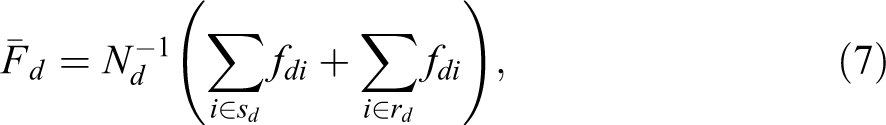
We consider the SAE problem for the mean under the EBLUP approach in the BHF model. Focusing on the population parameter of factor score means ${\bar{F}}_{d}, d = 1, \dots, D$ , and as the population mean is a linear quantity, we can write the following decomposition:

{\bar{F}}_{d} = N_{d}^{- 1} (\sum_{i \in s_{d}} f_{d i} + \sum_{i \in r_{d}} f_{d i}),

where f_di is the population factor score for unit i within small area d assuming that the factor model is implemented on the whole population.

When auxiliary variables are available at the unit level, the BHF model can be used in order to predict the out-of-sample units. Considering the data for unit i in area d being $(f_{d i}, x_{d i}^{T})$ where $x_{d i}^{T}$ denotes a vector of p auxiliary variables, the nested error regression model is the following:

\begin{array}{l} f_{d i} = x_{d i}^{T} β + u_{d} + e_{d i}, i = 1, \dots, N_{D}, d = 1, \dots, D, \\ u_{d} \sim iid N (0, σ_{u}^{2}), e_{d i} \sim iid N (0, σ_{e}^{2}), independent . \end{array}

In this model, there are two error components, u_d and e_di , the random effect and the residual error term, respectively.

According to Royall (1970), we can write the best linear unbiased predictor (BLUP) for the mean as follows:

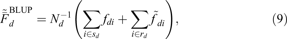
{\tilde{\bar{F}}}_{d}^{BLUP} = N_{d}^{- 1} (\sum_{i \in s_{d}} f_{d i} + \sum_{i \in r_{d}} {\tilde{f}}_{d i}),

where ${\tilde{f}}_{d i} = x_{d i}^{T} \tilde{β} + {\tilde{u}}_{d}$ is the BLUP of $f_{d i}$ , and ${\tilde{u}}_{d} = γ_{d} ({\bar{f}}_{d s} - {\bar{x}}_{d s}^{T} \tilde{β})$ the BLUP of u_d . Here, ${\bar{f}}_{d s} = n_{d}^{- 1} \sum_{i \in s_{d}} f_{d i}$ , ${\bar{x}}_{d s} = n_{d}^{- 1} \sum_{i \in s_{d}} x_{d i}$ , and $γ_{d} = \frac{σ_{u}^{2}}{σ_{u}^{2} + \frac{σ_{e}^{2}}{n_{d}}} \in (0, 1)$ . $γ_{d}$ is the shrinkage estimator measuring the unexplained between-area variability on the total variability.

Since in practice the variance components $σ_{e}^{2}$ and $σ_{u}^{2}$ are unknown, we replace these quantities by estimates, so we calculate the EBLUP of the mean:

{\hat{\bar{F}}}_{d}^{EBLUP} = N_{d}^{- 1} (\sum_{i \in s_{d}} f_{d i} + \sum_{i \in r_{d}} {\hat{f}}_{d i}),

where ${\hat{f}}_{d i} = x_{d i}^{T} \hat{β} + {\hat{u}}_{d}$ is the EBLUP of $f_{d i}$ . For details on $\hat{β}$ and ${\hat{u}}_{d}$ , we refer to Rao and Molina (2015). As shown in Rao and Molina (2015), ${\hat{\bar{F}}}_{d}^{EBLUP}$ can be also written as follows:

{\hat{\bar{F}}}_{d}^{EBLUP} = \frac{n_{d}}{N_{d}} {\bar{f}}_{d s} + {({\bar{X}}_{d p} - \frac{n_{d}}{N_{d}} {\bar{x}}_{d s})}^{T} \hat{β} + (1 - \frac{n_{d}}{N_{d}}) {\hat{u}}_{d} .

${\bar{X}}_{d p}$ denotes the means of the auxiliary variable in the population for the dth area.

If the sample size in a small area is zero, it holds that ${\hat{\bar{F}}}_{d}^{EBLUP} = {\bar{X}}_{d p} \hat{β} = {\hat{\bar{F}}}_{d}^{Synthetic}$ where ${\bar{X}}_{d p}$ denotes the means of the covariates in the population.

MSE Estimation

The MSE of equation (11) can be estimated via analytical approximations or resampling techniques. Prasad and Rao (1990) proposed an analytical approximation of MSE and González-Manteiga et al. (2008) proposed bootstrap techniques. Moreover, when large sample analytical approximations are available, the bootstrap might provide more accurate estimation alternatives to analytical approximations due to its second-order accuracy (González-Manteiga et al. 2008). Here, we suggest the use of a bootstrap method to estimate the MSE of equation (11). The bootstrap method proposed by González-Manteiga et al. (2008) has been adapted for the case of using factor score means as the dependent variable in the SAE models in order to take into account the variability arising from the factor analysis models. The steps are provided in Online Appendix A, and we evaluate our proposed algorithm via an extension to the simulation in Bootstrap MSE Estimation section. Analytical approximations of the MSE estimation of equation (11) under factor analysis models are a subject for future work.

Simulation Study

The simulation study was designed to assess the behavior of the EBLUP estimation of factor score means under a factor analysis model. We compare this approach with a weighted average of a dashboard of standardized univariate EBLUPs calculated from the original variables. We use a simple average and a weighted average where the weights are obtained by the factor loadings. We also assess the bootstrap MSE estimation for the EBLUP of factor score means which will be used in the application in Economic Well-being in Tuscany: A Multidimensional Approach section.

The simulation is based on generating one population and drawing 500 simple random samples without replacement (SRSWOR) which is a mixture between a design- and model-based simulation approach where model assumptions are generally met and we mainly focus on sample variability. Drawing SRSWOR random samples from the population will result in the real setting of unplanned domains (zero sample sizes) within our small areas. Although EU-SILC may have complex survey designs, one important feature in the Italian EU-SILC for Tuscany is that every household (and hence adult in the household) has an equal inclusion probability equal probability of selection method sampling (EPSEM) design, and hence, the simulation results based on an equal probability design are in line with the real data application. It is common to find in the literature other examples of simulation studies where simple random sampling is used to obtain unplanned domains, for example, Giusti et al. (2013) used this approach when investigating a range of estimators also based on the EU-SILC. The subject of complex survey designs in SAE is a topic of ongoing research.

Generating the Population

A single population is generated from a multivariate mixed-effects model, the natural extension of the BHF model (Fuller and Harter 1987) with N = 20,000, D = 80, and 130 ≤ N_d ≤ 420. N_d is generated from the discrete uniform distribution, $N_{d} \sim U (a = 130, b = 420)$ , with $\sum_{d = 1}^{D} N_{d} = 20, 000$ where the parameters are obtained from the Italian EU-SILC 2009 data set used in the application in Economic Well-being in Tuscany: A Multidimensional Approach section. Here, the multivariate model that we use to generate the population for the original variables (observed variables Y ) is:

\begin{array}{l} y_{d i} = x_{d i}^{T} β + u_{d} + e_{d i}, i = 1, \dots, N_{D}, d = 1, \dots, D, \\ u_{d} \sim iidMVN (0, Σ_{u}), e_{d i} \sim iidMVN (0, Σ_{e}), independent . \end{array}

$y_{d i}$ denotes a 3 × 1 vector of observed responses for unit i belonging to area d.

Two uncorrelated covariates are generated from the Normal distribution:

X_{1} \sim N (9.93, {4.98}^{2}), X_{2} \sim N (57.13, {17.07}^{2}) .

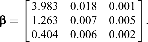
These parameters reflect two real variables in the Italian EU-SILC 2009 data set: the years of education and age (although we use here a normal [nontruncated] distribution). We selected K=3 response variables from the Italian EU-SILC 2009 data: the log of income, squared meters of the house, and the number of rooms, and fit regression models using the covariates X ₁ and X ₂.

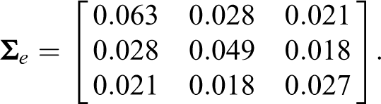
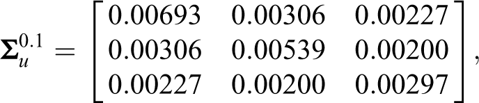
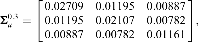
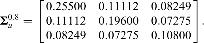
From these models, we estimate the β coefficient matrix and standard errors to build the simulation population by the model in equation (12). The $β (3 \times 3)$ matrix of coefficients is given by:

β = [\begin{matrix} 3.983 & 0.018 & 0.001 \\ 1.263 & 0.007 & 0.005 \\ 0.404 & 0.006 & 0.002 \end{matrix}] .

The response vector was generated according to the following variance components, where the correlation was set at 0.5 as derived from the Italian EU-SILC 2009 data:

Σ_{e} = [\begin{matrix} 0.063 & 0.028 & 0.021 \\ 0.028 & 0.049 & 0.018 \\ 0.021 & 0.018 & 0.027 \end{matrix}] .

We control the intraclass correlation (ICC) ρ defined as $ρ_{y_{k}} = σ_{u y_{k}}^{2} / (σ_{u y_{k}}^{2} + σ_{e y_{k}}^{2})$ , for the kth component of Y and obtain the variance–covariance matrices of the correlated random effects. We chose three levels of ICCs: 0.1, 0.3, and 0.8 and obtain the following matrices:

Σ_{u}^{0.1} = [\begin{matrix} 0.00693 & 0.00306 & 0.00227 \\ 0.00306 & 0.00539 & 0.00200 \\ 0.00227 & 0.00200 & 0.00297 \end{matrix}],

Σ_{u}^{0.3} = [\begin{matrix} 0.02709 & 0.01195 & 0.00887 \\ 0.01195 & 0.02107 & 0.00782 \\ 0.00887 & 0.00782 & 0.01161 \end{matrix}],

Σ_{u}^{0.8} = [\begin{matrix} 0.25500 & 0.11112 & 0.08249 \\ 0.11112 & 0.19600 & 0.07275 \\ 0.08249 & 0.07275 & 0.10800 \end{matrix}] .

We first estimate the factor analysis model on the population to derive the population factor scores $f_{i}, i = 1, \dots, N$ according to equation (4). These will be treated as true values in our simulation study.

We note that although factor analysis models have been developed for multilevel structures within domains, it is not possible to use these models for unplanned domains given a random sample due to small and zero sample size domains. Thus, two-level factor analysis models in SAE is a subject for future work.

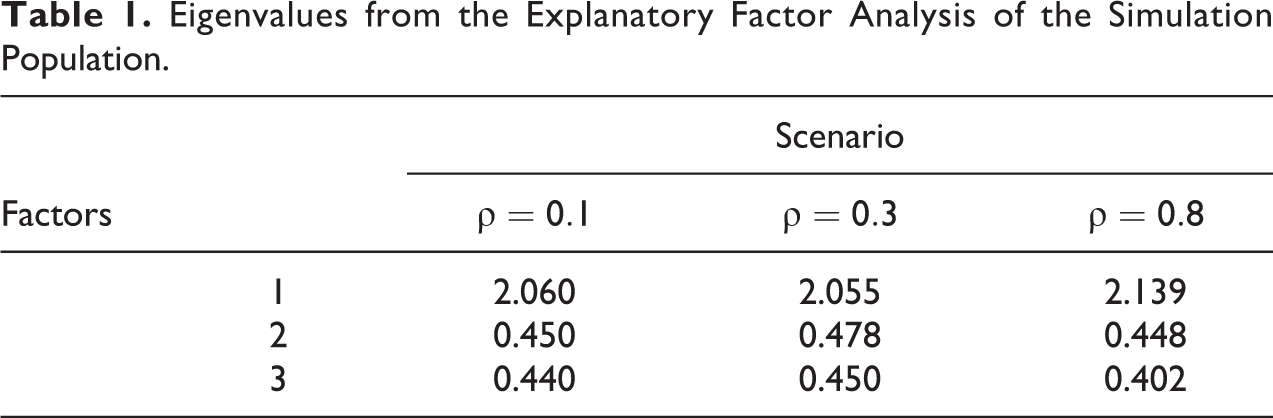
To derive the population factor scores, we first estimate an explanatory (unrestricted) factor analysis (EFA) model on the whole population, allowing for all possible factors. The EFA is estimated to check and identify the underlying relationships between observed variables (Norris and Lecavalier 2009). The EFA results show that the first factor explains a large amount of the total variability. Table 1 shows the estimated eigenvalues under different scenarios and Figure 1 the scree plots. The eigenvalue represents the variance of factor m and measures the variance in all the variables which is accounted for by that factor. With a large eigenvalue for the first factor, we then fit a one-factor CFA model on the population and estimate the population-based factor scores. The CFA one-factor model provides good fit statistics: root mean squared error of approximation (RMSEA = 0) and comparative fit index (CFI = 1), Tucker Lewis Index $[TLI = 1]$ (Hu and Bentler 1999).

Table 1.

Eigenvalues from the Explanatory Factor Analysis of the Simulation Population.

Factors		Scenario
Factors		$ρ = 0.1$	$ρ = 0.3$	$ρ = 0.8$
	1	2.060	2.055	2.139
	2	0.450	0.478	0.448
	3	0.440	0.450	0.402

Figure 1.

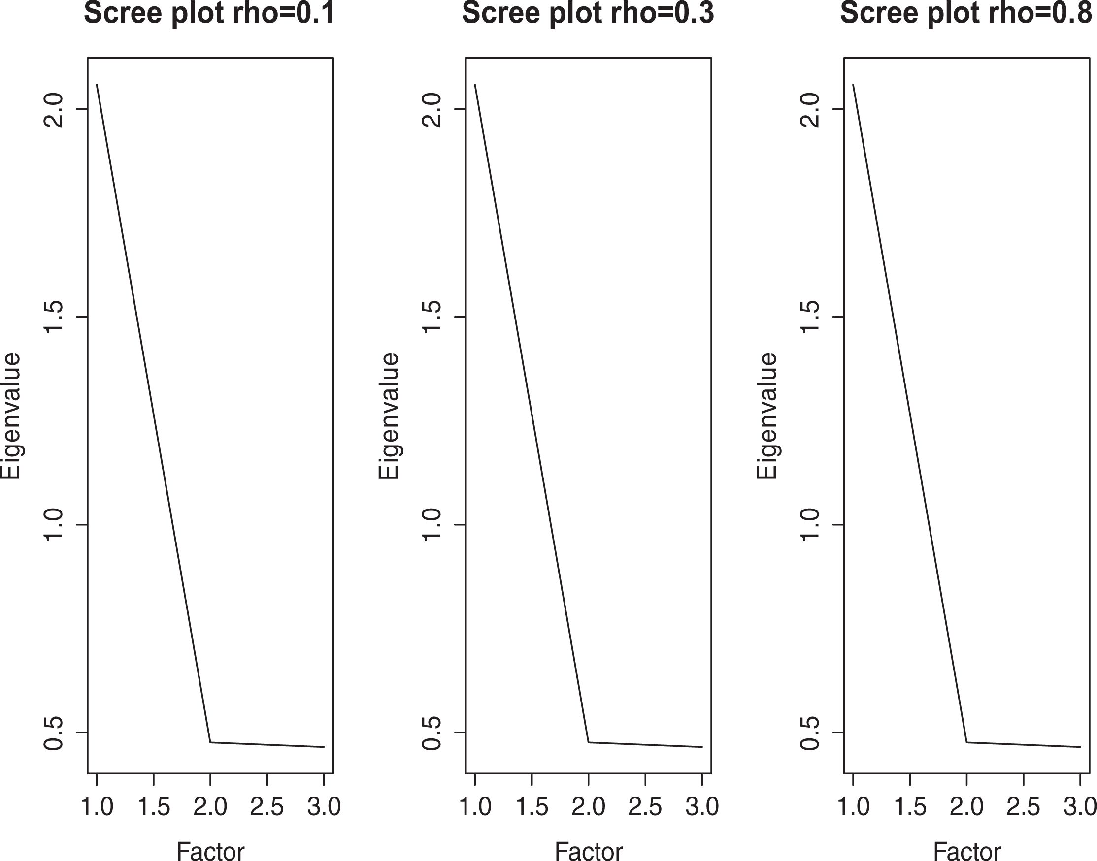
Scree plots from the explanatory factor analysis of the simulation population.

We now define the following “true” values for each of the small areas d from our simulated population for $i = 1, \dots, N$ , area $d = 1, \dots, D$ , and variables $k = 1, \dots, K$ :

the factor score means in area d: ${\bar{F}}_{d} = N_{d}^{- 1} \sum_{i} f_{d i}$ ,

simple average of the observed variable standardized means in area d: ${\bar{Y}}_{d}^{S_Averages} = \frac{\sum_{k = 1}^{K} {\bar{Y}}_{d k}^{*}}{K}$ ;

weighted average of the observed variables standardized means in area d using the factor loadings: ${\bar{Y}}_{d}^{W_Averages} = \frac{\sum_{k = 1}^{K} {\hat{λ}}_{k} {\bar{Y}}_{d k}^{*}}{\sum_{k = 1}^{K} {\hat{λ}}_{k}}$ .

${\bar{Y}}_{d k}^{*}$ denotes the standardized (mean zero and unit variance) true mean in area d and variable k where the standardization is obtained by subtracting the overall mean across all the areas and dividing by the standard deviation. ${\hat{λ}}_{k}$ denotes the estimated loading related to the kth variable in the population obtained from the above CFA.

We highlight again that under factor analysis model assumptions the factor scores are strongly linearly related to the observed variables and have the same economic interpretation as the observed variables.

Simulation Steps

The simulation study consists of the following steps:

draw S = 1,…,500 samples using simple random sampling without replacement (note that this results in unplanned domains with small or zero sample size);

fit the one-factor CFA model on each sample and estimate the EBLUP of factor score means for each area d in each sample. We also calculate Horvitz–Thompson (HT; Horvitz and Thompson 1952) direct estimates of the factor score means for those areas with a nonzero sample size. In addition, the EBLUP for each of the original variables is also estimated in order to construct a simple average of the standardized small area EBLUPs and a weighted average using the factor loadings;

As the true values are known from the simulation population, we are able to calculate the root mean squared error (RMSE) and the relative bias (RBIAS) for each area d for the three types of estimates: EBLUPs of factor score means and the simple and weighted average of EBLUPs. For example, for the EBLUPs of factor score means the RMSE is:

RMSE ({\hat{\bar{F}}}_{d}^{EBLUP}) = \sqrt{S^{- 1} {\sum_{s = 1}^{S} ({\hat{\bar{F}}}_{d s}^{EBLUP} - {\bar{F}}_{d})}^{2}},

and the RBIAS is:

RBIAS ({\hat{\bar{F}}}_{d}^{EBLUP}) = S^{- 1} \sum_{s = 1}^{S} \frac{({\hat{\bar{F}}}_{d s}^{EBLUP} - {\bar{F}}_{d})}{{\bar{F}}_{d}},

For the overall comparison across all areas, we rank the small areas according to the estimates averaged across the 500 samples and compare each to the ranking in the population. We also examine the average of the RMSE and RBIAS across all areas.

We estimate the EBLUP for each original variable separately on each of 500 samples, and then standardize them and construct weighted and simple averages. These are compared to the true values in the simulation population. The weighted mean in area d after standardizing the EBLUP estimates estimated on each sample s is given as follows:

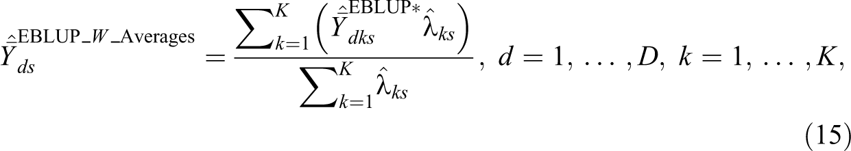
{\hat{\bar{Y}}}_{d s}^{EBLUP_W_Averages} = \frac{\sum_{k = 1}^{K} ({\hat{\bar{Y}}}_{d k s}^{EBLUP*} {\hat{λ}}_{k s})}{\sum_{k = 1}^{K} {\hat{λ}}_{k s}}, d = 1, \dots, D, k = 1, \dots, K,

where k denotes the kth variable and ${\hat{λ}}_{k s}$ the factor loading estimated on the sth sample for the kth variable, and the standardized EBLUP of the mean is calculated as follows: ${\hat{\bar{Y}}}_{d k s}^{EBLUP *} = ({\hat{\bar{Y}}}_{d k s}^{EBLUP} - M_{k s}^{EBLUP}) / S D_{k s}^{EBLUP}$ , where $M_{k s}^{EBLUP} = D^{- 1} {\sum_{d} \hat{\bar{Y}}}_{d k s}^{EBLUP}$ and $S D_{k s}^{EBLUP} = \sqrt{{(D - 1)}^{- 1} \sum_{d} {({\hat{\bar{Y}}}_{d k s}^{EBLUP} - M_{k s}^{EBLUP})}^{2}}$ .

In the following tables and figures, we dropped the subscript d as we show the estimates averaged across all small areas.

Results: Factor Scores versus Weighted and Simple Averages of Standardized EBLUPs

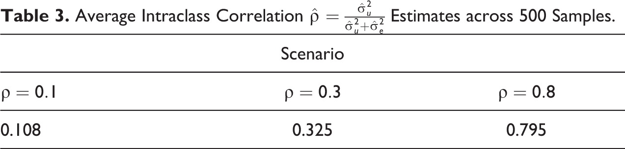
In this section, we show the main results of the simulation study. Table 2 contains the average eigenvalues across 500 samples under the EFA model and can be compared to Table 1 obtained from the simulation population. We can see that we are able to obtain good estimates for the eigenvalues across the samples. In parentheses, we show the ratios between the sample and population eigenvalues. Table 3 presents the ICC coefficients estimated from the SAE model (averaged across 500 samples) showing that we approximate the known ICC coefficients as defined in the simulation population.

Table 2.

Average Eigenvalues across 500 Samples from Explanatory Factor Analysis Model.

Factors		Scenario
Factors		$ρ = 0.1$	$ρ = 0.3$	$ρ = 0.8$
	1	2.058 (0.999)	2.050 (0.998)	2.135 (0.998)
	2	0.445 (0.989)	0.473 (0.990)	0.442 (0.987)
	3	0.442 (1.005)	0.455 (1.011)	0.405 (1.007)

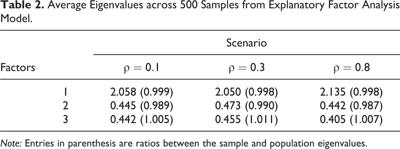
Note: Entries in parenthesis are ratios between the sample and population eigenvalues.

Table 3.

Average Intraclass Correlation $\hat{ρ} = \frac{{\hat{σ}}_{u}^{2}}{{\hat{σ}}_{u}^{2} + {\hat{σ}}_{e}^{2}}$ Estimates across 500 Samples.

Scenario
$ρ = 0.1$	$ρ = 0.3$	$ρ = 0.8$
0.108	0.325	0.795

For each of the three estimates in small area d averaged across the 500 samples, we compare the ranking of the small area domain estimates with the true ranking based on true area means according to our simulation population using a Spearman’s correlation coefficient. These are shown in Table 4. The EBLUPs of the factor score means show an improvement and higher correlation to the true means in the population compared to the averages of EBLUPs, especially for the case of ρ = 0.1.

Table 4.

Spearman’s Correlation Estimates for the Three Approaches.

Approach	Scenario
Approach	$ρ = 0.1$	$ρ = 0.3$	$ρ = 0.8$
${\hat{\bar{Y}}}^{E B L U P_S_A v e r a g e s}$	.780	.996	.999
${\hat{\bar{Y}}}^{E B L U P_W_A v e r a g e s}$	.793	.996	.998
${\hat{\bar{F}}}^{E B L U P}$	.986	.997	.999

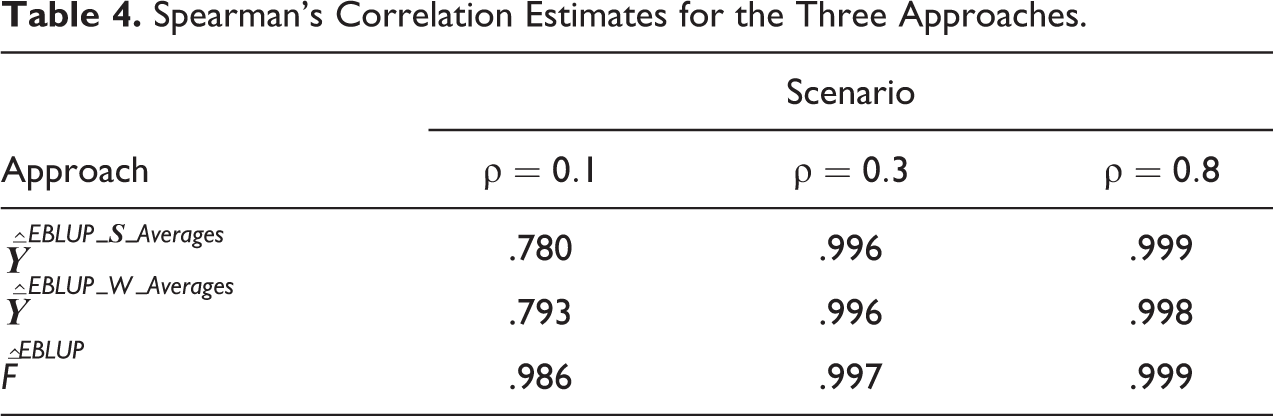
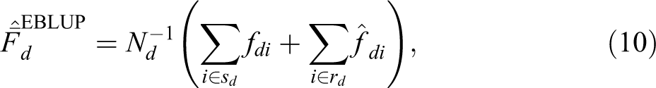
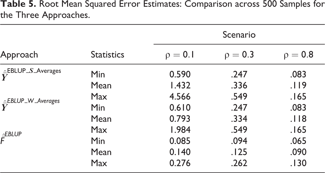
Figure 2 shows the individual RMSE of the small areas for those areas with nonzero sample sizes. In line with the SAE literature, the EBLUP approach produces estimates with lower variability than direct HT estimates. Table 5 shows the overall RMSE comparison defined in (10) across 500 samples for the EBLUPs of factor scores and simple and weighted standardized EBLUPs. We do not show the overall RBIAS across the samples and areas since the estimates are all unbiased. 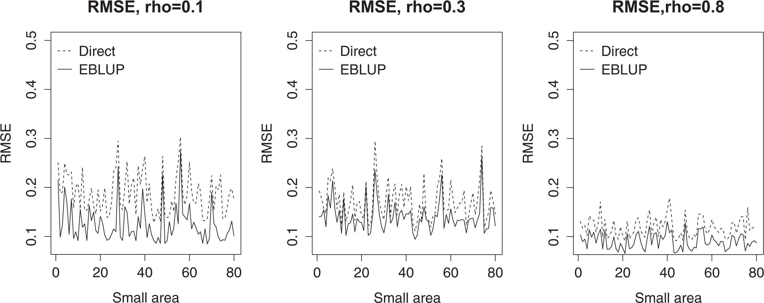In contrast to Figure 2, Table 5 presents the minimum, mean, and maximum RMSE across all areas including those areas that had zero sample size and hence the synthetic estimator ${\hat{\bar{F}}}_{d}^{Synthetic} = {\bar{X}}_{d p} \hat{β}$ where ${\bar{X}}_{d p}$ denotes the means of the covariates in the population is used as the final estimator. The maximum values in Table 5 are generally obtained for those areas with zero or very small sample sizes. The larger the sample size, the smaller the RSME. The overall RMSEs for the EBLUP factor score means are lower than in the case of the simple and weighted averages of the dashboard of single EBLUPs for all levels of ICCs, even after taking into account the extra modeling step of estimating factor scores. Hence, applying the EBLUP method on factor score means provides more precise estimates while reducing the data dimensionality of multiple observed variables.

Figure 2.

Root mean squared error for direct estimates and empirical best linear unbiased prediction of factor score means for small areas with n_d > 0.

Table 5.

Root Mean Squared Error Estimates: Comparison across 500 Samples for the Three Approaches.

		Scenario
Approach	Statistics	$ρ = 0.1$	$ρ = 0.3$	$ρ = 0.8$
${\hat{\bar{Y}}}_{}^{EBLUP_S_Averages}$	Min	0.590	.247	.083
	Mean	1.432	.336	.119
	Max	4.566	.549	.165
${\hat{\bar{Y}}}_{}^{E B L U P_W_A v e r a g e s}$	Min	0.610	.247	.083
	Mean	0.793	.334	.118
	Max	1.984	.549	.165
${\hat{\bar{F}}}_{}^{E B L U P}$	Min	0.085	.094	.065
	Mean	0.140	.125	.090
	Max	0.276	.262	.130

Bootstrap MSE Estimation

In the application, we will use the algorithm defined in Online Appendix A to estimate the MSE of the EBLUP of the factor score means using a modified parametric bootstrap which take into account the variability arising from the factor analysis model. We extend here the simulation for the case of the ICC of 0.3 to assess the properties of our proposed bootstrap MSE estimation.

We compare the bootstrap RMSE according to the algorithm in Online Appendix A with the empirical RMSE (ERMSE) obtained across the 500 samples calculated as ERMSE. We consider the ERMSE as the “true” MSE and assess whether our proposed modified parametric bootstrap MSE estimator is unbiased.

Figure 3 shows the ratio between the parametric bootstrap RMSE averaged across the 500 samples under two settings: (1) treating the factor scores as fixed and (2) accounting for the variability of the factor analysis model, against the ERMSE. It can be seen that the RMSE estimated via parametric bootstrap without accounting for the factor model is underestimated with an RBIAS of −34.6 percent across the small areas. However, the RBIAS across the small areas when accounting for the variability in the factor analysis model is negligible at 4.0 percent.

Figure 3.

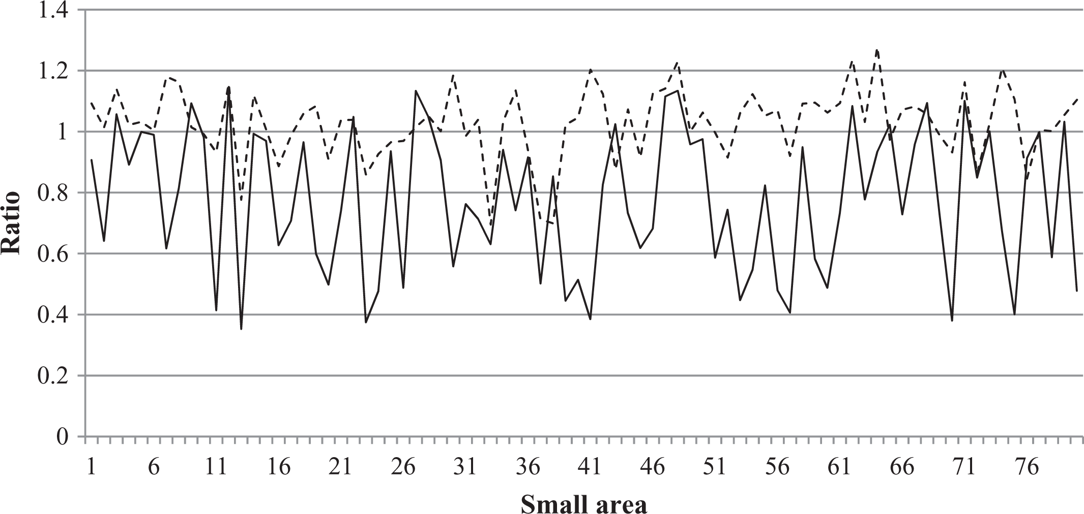
Ratios between bootstrap root mean squared error (RMSE) and empirical RMSE estimated via bootstrap taking into account the factor analysis model variability (---) and bootstrap ignoring the factor analysis model variability (__).

To illustrate this point further, Figure 4 presents the coverage rate comparisons of the parametric bootstrap estimated MSE taking into account the factor analysis model variability and ignoring the factor analysis model variability. There are significantly smaller coverage rates if we ignore the factor analysis model variability. The coverage rate when taking the variability into account is relatively stable at 95 percent.

Figure 4.

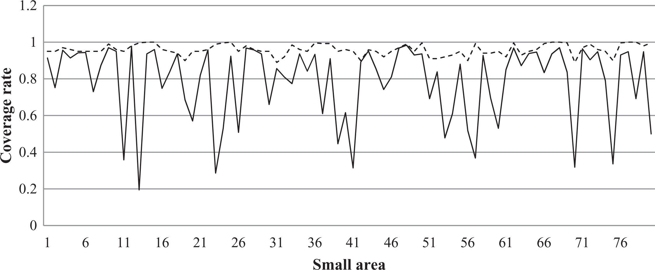
Coverage rates comparisons: bootstrap root mean squared error estimated taking into account the factor analysis model variability (---) and bootstrap ignoring the factor analysis model variability (__).

Therefore, we conclude from this extension to the simulation study that treating the factor scores as fixed in the standard parametric bootstrap approach leads to a severe underestimation in the RMSE and our modified parametric bootstrap in Online Appendix A performs well.

Final Remarks of the Simulation Study

The use of factor scores provides better rankings to true values compared to weighted and simple averages of single variables, especially for the case of small ICCs which are more common in real settings. Furthermore, it can be seen that factor scores provide estimates with lower variability (in terms of RMSE) than weighted and simple averages of single variables for estimating multidimensional phenomena at the small area level. We also conclude that it is crucial to consider the variability arising from the factor analysis model in the parametric bootstrap MSE estimation; otherwise, the true MSE will be underestimated.

Based on these results, we use the EBLUP of the factor score means approach to reduce the dimensionality of observed variables in a real application using the Italian 2009 EU-SILC data for the Tuscany region and the modified parametric bootstrap procedure for MSE calculations in Economic Well-being in Tuscany: A Multidimensional Approach section.

Economic Well-being in Tuscany: A Multidimensional Approach

The aim of this section is to demonstrate how we can provide estimates of an economic well-being indicator following the BES guidelines for Tuscany municipalities. In our application, we use data from the EU-SILC 2009 and the 2001 General Census of Population and Housing. We note that the EU-SILC 2009 data were collected several years after the census and this is a limitation of the study since we assume stationarity of growth between the periods. Obviously, the economic and financial crisis occurring in 2008 violates this assumption and further studies are needed with more current covariates. Nevertheless, the application is useful to demonstrate how small area estimates can be calculated for a multidimensional indicator. The specification of the main R functions used in this analysis are presented in Online Appendix C.

Data and Variables

Income and economic resources can be seen as conditions by which an individual is able to have a sustainable standard of life. One of the dimensions in the Italian Equitable and Sustainable Well-being (BES) framework is dedicated to economic well-being (ISTAT 2015). It consists of 10 single economic-related indicators (a dashboard of indicators). In this work, we focus on a subset of these highly correlated variables:

severe material deprivation according to Eurostat;

equivalized disposable income;

housing ownership;

housing density.

Online Appendix B in Figure B1 contains the variables nomenclature for the 2009 Tuscany EU-SILC data set used in our study and descriptive statistics of these study variables which are explained in the next sections.

Material deprivation can be defined as the inability to afford some items considered to be desirable, or even necessary, to achieve an adequate standard of life. Indicators related to this are absolute measures useful to analyze and compare aspects of poverty in and across EU countries (Eurostat 2012). According to Eurostat, material deprivation in the EU can be measured by the proportion of people whose living conditions are severely affected by a lack of basic resources. Technically, the severe material deprivation rate shows the proportion of people living in households that cannot afford at least four of the following nine items because of financial difficulty:

mortgage or rent payments, utility bills, hire purchase installments, or other loan payments;

one-week holiday away from home;

a meal with meat, chicken, fish, or vegetarian equivalent every second day;

unexpected financial expenses;

a telephone (including mobile telephone);

a color TV;

a washing machine;

a car;

heating to keep the home sufficiently warm.

It can be argued that some of these indicators (e.g., 5 and 6) are nowadays less relevant than in the past. Nevertheless, these indicators are still used to describe the difficulties that households face in achieving a standard of life considered to be sufficient by society. This index is described in Table B3 in Online Appendix B. Disposable household income is the sum of gross personal income components plus gross income components at the household level minus employer’s social insurance contributions, interest paid on mortgage, regular taxes on wealth, regular interhousehold cash transfer paid, and tax on income. In order to take into account differences in household size and composition, we consider disposable equivalized income I^DE defined as follows:

I_{i}^{D E} = \frac{I_{i}^{D}}{n_{i}^{E}}, i = 1, \dots, N,

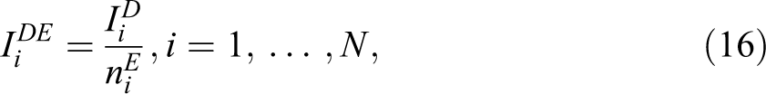
where i = 1,…, n denotes households, $I_{i}^{D}$ is the disposable household income, and $n_{i}^{E}$ is the equivalized household size calculated in the following way (Haagenars, Klaas, and Zaidi 1994):

n_{i}^{E} = 1 + 0.5 \cdot (H M_{14 +} - 1) + 0.3 \cdot H M_{13 -},

where HM ₁₄₊ and HM ₁₃₊ are the numbers of household members aged 14 and over and 13 or younger at the end of the income reference period, respectively. This so-called OECD modified scaling procedure is crucial to taking into account the economy of scales in the household. Due to the skewness of the variable, we use the log transformation in the factor model and SAE. The histograms are in Figure B2 and descriptive statistics in Table B1 of Online Appendix B. Housing ownership is measured by a dichotomous variable (0,1) where 0 denotes that the property where the household lies is not owned. According to the 2009 Tuscany EU-SILC data, 73.96 percent of households own the property where they live (see Table B3 in Online Appendix B). Overcrowding is one of the indicators that National Statistics Institutes include in their well-being measurement frameworks. A very simple indicator of housing density is given by the ratio between the number of rooms in the household (excluding kitchen, bathroom, and rooms used for work purposes) and the household size:

{\bar{r}}_{i} = \frac{R_{i}}{M_{i}},

where i is the household, M_i denotes the number of people in the ith household, and R_i the number of rooms in the household. The histogram of this variable is in Figure B3 and descriptive statistics are in Table B2 of Online Appendix B.

EU-SILC is conducted yearly by ISTAT for Italy and coordinated by EUROSTAT at the EU level. The survey is designed to produce accurate estimates at the national and regional levels (NUTS-2).

Hence, for the Italian geography, the survey is not representative of provinces, municipalities (NUTS-3 and LAU-2 levels, respectively), and lower geographical levels. The regional samples are based on a stratified two-stage sample design. The primary sampling units (PSUs) are the municipalities within the provinces, and households are the secondary sampling units (SSUs). The PSUs are stratified according to their population size and SSUs are selected by systematic sampling in each selected PSU. Each household has an equal probability of selection. The total number of households in the sample for Tuscany is 1,448.

The 14th Population and Housing Census 2001 surveyed 1,388,252 households of persons living in Tuscany permanently or temporarily, including the homeless population and persons without a dwelling.

The Construction of the Factor Scores

The one-factor analysis model described in Using Factor Scores for Data Dimensionality Reduction section is fitted, and according to the goodness-of-fit statistics estimated on the one-factor model solution, the RMSEA = 0.047 and the CFI criteria (CFI = 0.966), the model provides good fit (Hu and Bentler 1999). This choice can be justified also substantively as our variables relate to economic well-being according to the BES framework, which is the phenomenon we want to measure.

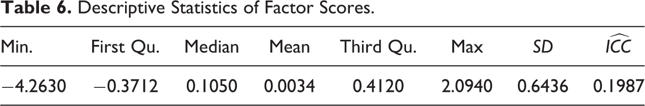
The histogram, Q–Q plot, and box-plot of the factor scores are shown in Figure 5 as well as descriptive statistics in Table 6. We see evidence of a slight skewness in the factor scores likely due to discrete variables included in the factor analysis model. One interesting thing to note based on Table B4 in Online Appendix B is that the estimated ICC for the factor scores is 0.1987 which is considerably higher than the estimated ICCs for the single study variables; thus as seen in the simulation study, we expect that the EBLUP of the factor scores will provide good rankings of the small areas compared to weighted and simple averages.

Figure 5.

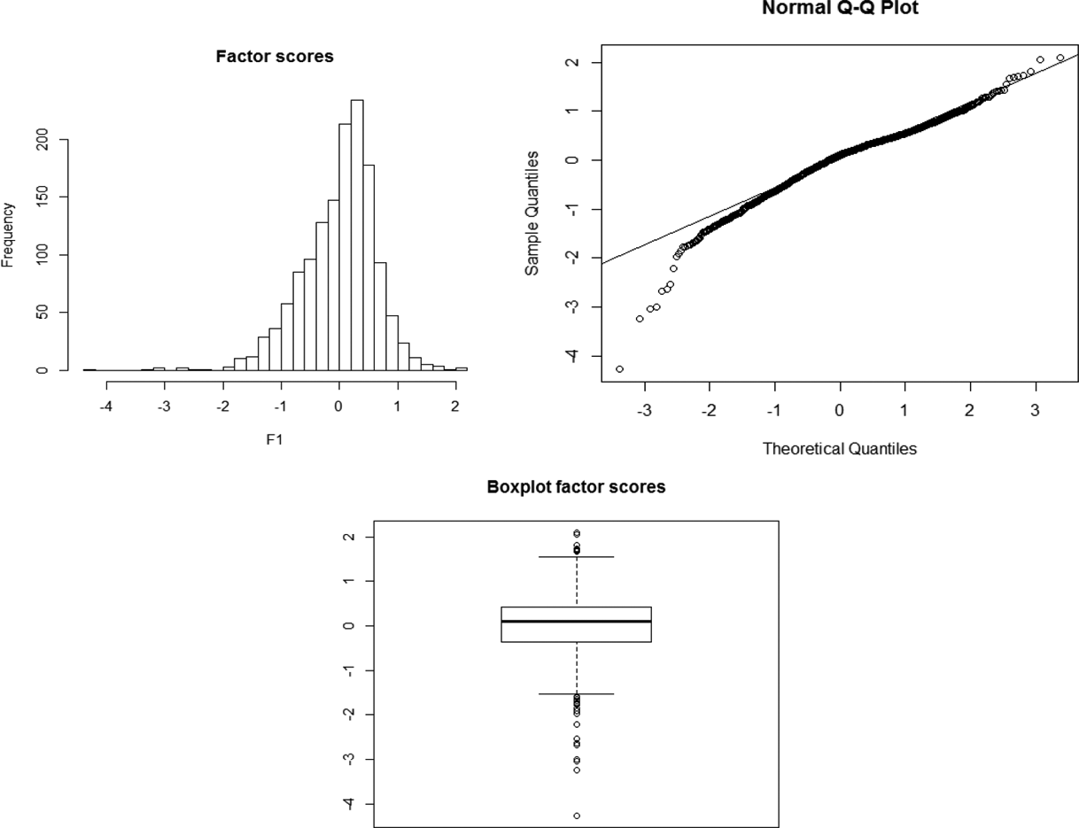
Factor scores distribution graphs.

Table 6.

Descriptive Statistics of Factor Scores.

Min.	First Qu.	Median	Mean	Third Qu.	Max	SD	$\hat{I C C}$
−4.2630	−0.3712	0.1050	0.0034	0.4120	2.0940	0.6436	0.1987

Small Area Estimates

In this application, we treat municipalities as our small areas of interest. The municipalities within Tuscany are unplanned domains in EU-SILC and only 59 of 287 were sampled. Sample sizes in municipalities range from 0 to 135 households.

First, we provide direct estimates for the small areas with $n_{d} > 0$ . After this, we build an SAE model under the BHF approach where the response variable is the factor score interpreted as the latent economic well-being construct. The exploratory variables in the model relate to the head of the household and are those common to both the survey and Census data. In particular, after a preliminary analysis of the available data, we chose gender, age, year of education, household size, size of the flat (in squared meters), and employment status as the explanatory variables.

The single EBLUPs of the dashboard indicators have been estimated to construct the simple and weighted averages, as was done in the simulation study. In the case of binary variables, the following linear logistic mixed effects model was fitted (MacGibbon and Tomberlin 1989):

logit (p_{d i}) = log (\frac{p_{d i}}{1 - p_{d i}}) = x_{d i}^{T} β + u_{d},

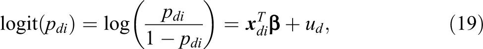
where p_di is the probability that $y_{d i} = 1$ and $u_{d} \sim iid N (0, σ_{u}^{2})$ .

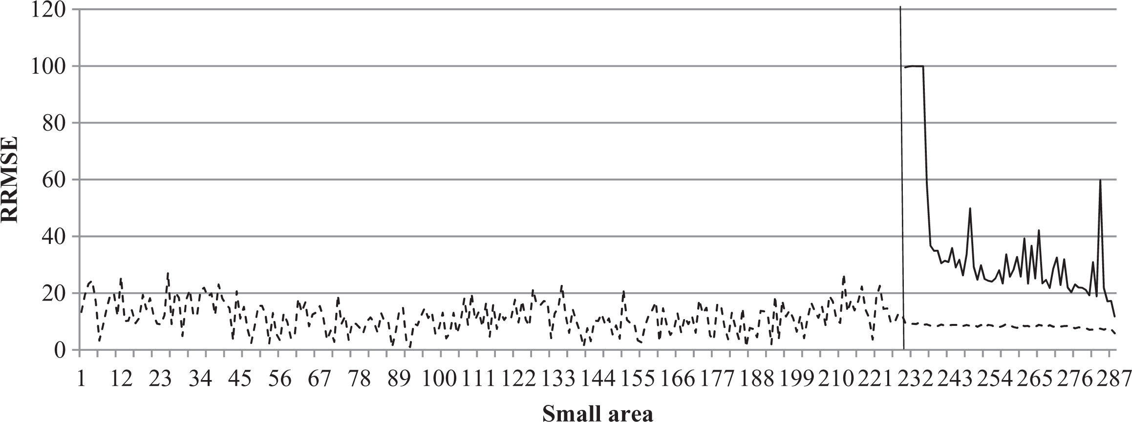
In Figure 6, we compare the relative root mean squared error (RRMSE) of the EBLUPs of factor score means with the coefficients of variation of the direct estimates for the sampled areas (to the right of the vertical line). We also include in Figure 6 the RRMSE for the nonsampled areas where $n_{d} = 0$ (to the left of the vertical line). Here, the estimates of the MSE for the predictions are obtained via the modified parametric bootstrap with $B = 500$ bootstrap samples as described in Online Appendix A. We can see the gain in efficiency (in terms of reduction in the RRMSE) obtained by the EBLUP compared to the direct estimates and in particular the RRMSEs are below 10 percent. In addition, even when the synthetic estimators are used in those areas with zero sample sizes, we still obtain an RRMSE that is below 20 percent. We note that an estimator with an RRMSE below 20 percent are considered reliable estimates (Australian Bureau of Statistics 2015).

Figure 6.

Relative root mean squared error direct estimates (__) and empirical best linear unbiased predictions (---) ordered by growing sample size.

To facilitate the interpretation and provide a comparison between the different economic well-being indicators obtained from the EBLUP factor score means and the simple and weighted averages of the dashboard of EBLUPs, we have normalized the EBLUPs using the “Min-Max” method (OECD-JRC 2008), with range [0, 1]. For the factor score EBLUPs, the normalization (denoted with a “*”) is as follows:

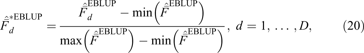
{\hat{\bar{F}}}_{d}^{*EBLUP} = \frac{{\hat{\bar{F}}}_{d}^{EBLUP} - min ({\hat{\bar{F}}}_{}^{EBLUP})}{max ({\hat{\bar{F}}}_{}^{EBLUP}) - min ({\hat{\bar{F}}}_{}^{EBLUP})}, d = 1, \dots, D,

where ${\hat{\bar{F}}}_{}^{EBLUP} = {col}_{1 \leq d \leq D} {\hat{\bar{F}}}_{d}^{EBLUP}$ . And similarly, for the simple and weighted averages of the dashboard of standardized EBLUPs.

Table 7 shows the percentiles for the latent economic well-being indicator based on the normalized EBLUP factor scores and the normalized averages of the dashboard of EBLUPs. Figures 7 and 8 depict the maps of the quartiles of the EBLUPs under the different approaches for the Tuscany region.

Table 7.

Percentiles for the Transformed Latent Economic Well-being Indicator Based on the Empirical Best Linear Unbiased Prediction (EBLUP) of Factor Score Means and Simple and Weighted Averages.

Percentile	0%	25%	50%	75%	100%
EBLUP	.0000	.5110	.5468	.5819	1.0000
Simple	.0000	.4297	.5297	.6061	1.0000
Weighted	.0000	.4796	.6006	.7184	1.0000

Figure 7.

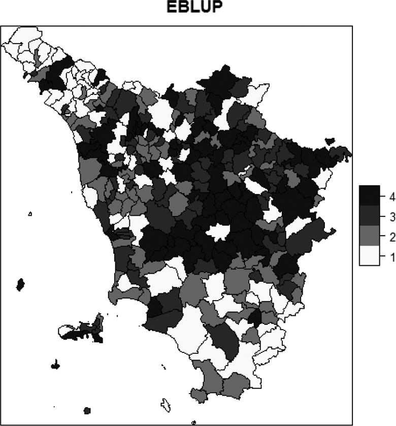
Latent economic well-being indicator based on transformed empirical best linear unbiased prediction of factor scores means (1 = first quartile, 2 = second quartile, 3 = third quartile, 4 = fourth quartile).

Figure 8.

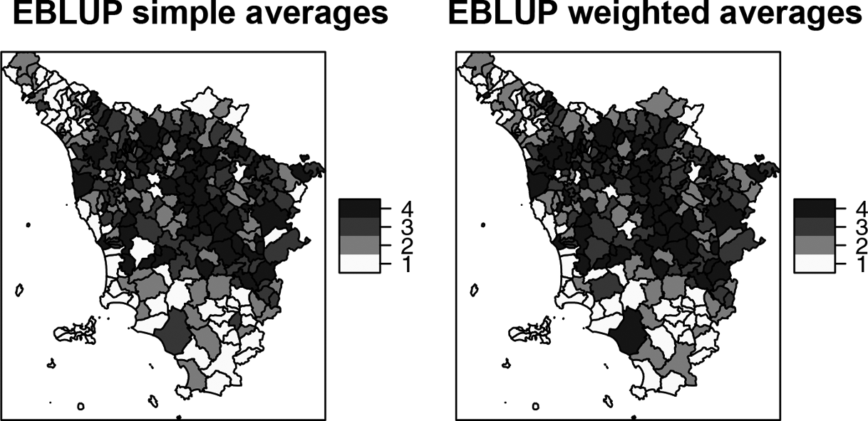
Latent economic well-being indicator based on simple and weighted averages of single empirical best linear unbiased predictions (1 = first quartile, 2 = second quartile, 3 = third quartile, 4 = fourth quartile).

In the maps of Figures 7 and 8, a darker color denotes a better well-being phenomenon. Looking at these figures, we can draw some interesting conclusions on economic well-being in the Tuscany region.

The municipalities located in the Massa-Carrara province, which is based in the North of Tuscany (i.e., Pontremoli and Zeri municipalities), and municipalities based in Grosseto province (south of Tuscany), are the poorest ones. The small areas based in the Florence province are wealthy municipalities, as well as the ones located in the center of the region (Siena province). The lowest point estimates of the latent economic well-being indicator are estimated for Carrara and Seravezza municipalities and the highest values for Firenze and Arezzo municipalities. Our results based on the EBLUPs of the factor scores in Figure 7 are more comparable with other SAE studies on welfare and poverty in Tuscany (Giusti et al. 2015; Marchetti, Tzavidis, and Pratesi 2012) compared to the averages of a dashboard of EBLUPs in Figure 8, though previous SAE studies consider only income variables rather than a composite indicator used here. This is not surprising given the low ICCs for each of the individual EBLUPs that form the dashboard which may result in more distortions on the rankings, particularly since some of the individual EBLUPs are based on discrete variables.

Model Diagnostics

We assess the fit of the model by analyzing the level-1 and level-2 standardized residuals. In particular, the Q–Q plots of the residuals, shown in Figures 9 and 10, show the leverage measures versus standardized scaled residuals from the linear model. Both figures show a presence of outliers in the left tail, although the factor scores distribution is approximately symmetric. Figure 10 also shows the contour of the Cook’s distance which does not deviate much from zero, and hence, we can conclude that the outliers are not influential.

Figure 9.

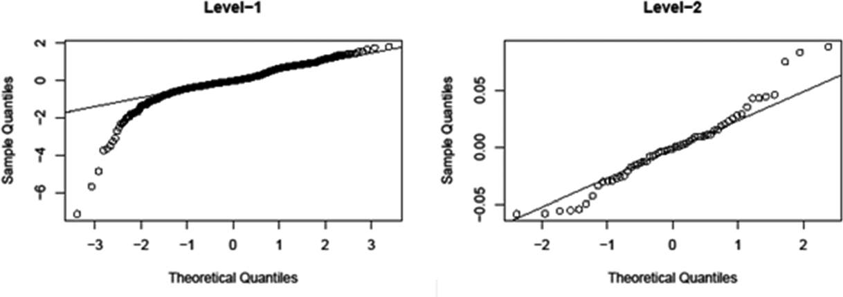
Q–Q plots for the level 1 and level 2 residuals of the Battese, Harter, and Fuller model fitting.

Figure 10.

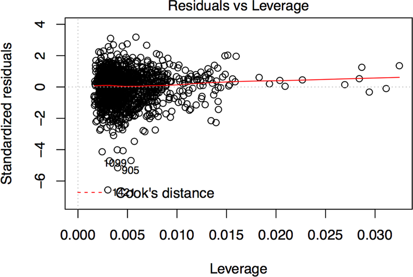
Standardized residuals versus leverage measure.

Conclusion and Discussion

In this article, we evaluated a method to estimate the mean of a latent economic well-being indicator at the local level for Tuscany using factor scores to reduce data dimensionality. We focused on the factor scores because they can be seen as a latent economic well-being composite variable. The simulation study demonstrated that factor score means provide a better ranking of the small areas compared to the true population means as measured by the Spearman’s correlation coefficient, especially when ICCs are small, which is common in real settings. The simple and weighted averages of univariate standardized EBLUPs also provide good rankings for the higher ICCs that were examined. In addition, the use of factor scores provided more precise estimates in terms of the MSE for an estimate of a multidimensional phenomenon compared to the averages of the EBLUPs. The use of factor analysis models and factor scores has important advantages and implications in data dimensionality reduction: it avoids arbitrary weighting of single indicators and it generates continuous composite scores, which can be modeled using model-based SAE methods. Since the factor scores are strongly linearly related to the multidimensional observed variables, this leads to easier interpretation.

Another important point studied in this article is the MSE estimation of EBLUPs of factor score means. In this work, we proposed a modification to the González-Manteiga et al. (2008) parametric bootstrap algorithm to account for the additional variability added to the small area estimates by using factor scores obtained from a factor analysis model as the dependent variable. This has been tested via simulation and we showed that if the variability arising from the factor analysis model is ignored, the MSE is underestimated and therefore biased. For more theoretical details on the bootstrap, we refer to González-Manteiga et al. (2008). Analytical MSE approximations are left for future work.

There are several areas where this work could be extended. Future work might consider other geographical levels, such as Sistemi Locali del Lavoro—Labor Local System, by looking at the flow of daily travel home/work (commuting) detected during the General Census of Population and Housing. Further interesting applications would involve comparisons between Italian regions in the North, Central, and South.

Another worthwhile extension is accounting for more than one factor. When the goal is to reduce the dimensionality of the original data by identifying latent factors, one might face the issue of identifying multiple factors. Multiple latent factors can arise, particularly when we have many indicators referring to the same phenomenon which can be grouped substantively into subdomains. For example, if the goal is to study housing quality, we may want to consider the following dimensions: type of dwelling and tenure status, housing affordability, and housing quality (e.g., overcrowding, housing deprivation, problems in the residential area). For multiple latent factors, we may have factor scores that are correlated, and hence, future research should explore the use of the multivariate mixed effects model (Fuller and Harter 1987). Datta, Day, and Basawa (1999) showed that the use of the multivariate mixed effects model might lead to gains in efficiency in terms of MSE for the EBLUP compared to the BHF model. Therefore, the multivariate SAE method might provide better dashboard estimates and averages if the correlation between the single variables is taken into account. These extensions are currently being carried out in Moretti, Shlomo, and Sakshaug (2017).

Supplemental Material

Supplemental Material, Appendices_SMR_826160 - Small Area Estimation of Latent Economic Well-being

Supplemental Material, Appendices_SMR_826160 for Small Area Estimation of Latent Economic Well-being by Angelo Moretti, Natalie Shlomo, and Joseph W. Sakshaug in Sociological Methods & Research

Footnotes

Declaration of Conflicting Interests

The author(s) declared no potential conflicts of interest with respect to the research, authorship, and/or publication of this article.

Funding

The author(s) disclosed receipt of the following financial support for the research, authorship, and/or publication of this article: This work was supported by Economic and Social Research Council (ES/J500094/1).

ORCID iD

Angelo Moretti

Supplemental Material

Supplemental material for this article is available online.

References

Australian Bureau of Statistics. 2015. “Survey of Disability, Ageing and Carers, 2012. Modelled Estimates for Small Areas, Projected 2015.” Retrieved April 30, 2017 (https://www.health.gov.au/internet/main/publishing.nsf/Content/98DCE47FC10BDD51CA257F15000413F5/$File/SDAC%202012%20Modelled%20Estimates%20for%20Small%20Areas%20projected%202015_Explanatory%20Notes%20-%20Release%201.pdf).

Bartholomew

David J.

Deary

Ian J.

Lawn

Martin

. 2009. “The Origin of Factor Scores: Spearman, Thomson and Bartlett.” British Journal of Mathematical and Statistical Psychology 62:569–82.

Bartholomew

David J.

Steele

Fiona

Moustaki

Irini

Galbraith

Jane I.

. 2008. Analysis of Multivariate Social Science Data. New York: Chapman & Hall/CRC Statistics in the Social and Behavioural Sciences Series.

Battese

George. E.

Harter

Rachel M.

Fuller

Wayne A.

. 1988. “An Error-components Model for Prediction of County Crop Areas Using Survey and Satellite Data.” Journal of the American Statistical Association 83(401):28–36.

Bell

Sherry M.

McCallum

Steve R.

Cox

Elizabeth

. 2003. “Toward a Research-based assessment of Dyslexia: Using Cognitive Measures to Identify Reading Disabilities.” Journal of Learning Disabilities 36(6):505–16.

Betti

Gianni

Gagliardi

Francesca

. 2017. “Extension of JRR Method for Variance Estimation of Net Changes in Inequality Measures.” Social Indicators Research 137(1):45–60.

Betti

Gianni

Gagliardi

Francesca

Verma

Vijay

. 2017. “Simplified Jackknife Variance Estimates for Fuzzy Measures of Multidimensional Poverty.” International Statistical Review 86(1):68–86.

Datta

Gauri S.

Day

Bannmo

Basawa

Ishwar

. 1999. “Empirical Best Linear Unbiased and Empirical Bayes Prediction in Multivariate Small Area Estimation.” Journal of Statistical Planning and Inference 75:269–79.

DiStefano

Christine

Zhu

Min

Mindrila

Diana

. 2009. “Understanding and Using Factor Scores: Considerations for the Applied Researcher.” Practical Assessment, Research and Evaluation 14(20):1–11.

10.

Eurostat. 2012. “Measuring Material Deprivation in the EU.” Methodologies and Working papers, 2012. Retrieved February 13, 2017 (http://ec.europa.eu/eurostat/documents/3888793/5853037/KS-RA-12-018-EN.PDF/390c5677-90a6-4dc9-b972-82d589df77c2).

11.

Ferro Luzzi

Giovanni

Fluckiger

Yves

Weber

Sylvain

. 2008. A Cluster Analysis of Multidimensional Poverty in Switzerland in Kakwani, Nanak. and Jacques Silber. 2008. Quantitative Approaches to Multidimensional Poverty Measurement. Basingstoke, England: Palgrave Macmillan.

12.

Fuller

Wayne A.

Harter

Rachel M.

. 1987. “The Multivariate Components of Variance Model for Small Area Estimation.” Pp. 103–23 in Small Area Statistics, edited by Richard

Platek

Rao

J. N. K.

Sarndal

Carl-Erik.

Singh

M. P.

. New York: Wiley.

13.

Gasparini

Leonardo

Escudero

Walter Sosa

Marchionni

Mariana

Olivieri

Sergio

. 2011 “Multidimensional Social Poverty in Latin America and the Caribbean: New Evidence from the Gallup World Poll.” Journal of Economic Inequality 11(2):1–20.

14.

Giusti

Caterina

Masserini

Lucio

Pratesi

Monica

. 2015. “Local Comparisons of Small Area Estimates of Poverty: An Application within the Tuscany Region of Italy.” Social Indicators Research 131(1):1–20.

15.

Giusti

Caterina

Tzavidis

Nikos

Pratesi

Monica

Salvati

Nicola

. 2013. “Resistance to Outliers of M-Quantile and Robust Random Effects Small Area Models.” Communications in Statistics—Simulations and Computations 43(3):549–68.

16.

González-Manteiga

Wenceslao

Lombardía

Maria J.

Molina

Isabel

Morales

Domingo

Santamaría

Laureano

. 2008. “Bootstrap Mean Squared Error of a Small-area EBLUP.” Journal of Statistical Computation and Simulation 78:443–62.

17.

Haagenars

Aldi J. M.

Klaas

de Vos

Zaidi

Ashar

. 1994. Poverty Statistics in the Late 1980s: Research Based on Micro-data. Luxembourg, Europe: Office for Official Publications of the European Communities.

18.

Hershberger

Scott L.

2005. “Factor Scores.” Pp. 636–44 in Encyclopedia of Statistics in Behavioral Science, edited by Everitt

B. S.

Howell

D. C.

. New York: John Wiley.

19.

Horvitz

Daniel G.

Thompson

Donovan J.

. 1952. “A Generalization of Sampling without Replacement from Finite Universe.” Journal of the American Statistical Association 47:663–85.

20.

Litze

Bentler

Peter M.

. 1999. “Cutoff Criteria for Fit Indexes in Covariance Structure Analysis: Conventional Criteria versus New Alternatives.” Structural Equation Modeling 6(1):1–55.

21.

Härdle

Wolfgang K.

Simar

Léopold

. 2012. Applied Multivariate Statistical Analysis. Verlag Berlin Heidelberg: Springer.

22.

ISTAT. 2015. “BES 2015. Il benessere equo e sostenibile in Italia.” Report by ISTAT and CNEL in 2015. (http://www.istat.it/it/files/2015/12/Rapporto_BES_2015.pdf In Italian).

23.

Johnson

Richard A.

Wichern

Dean W.

. 1998. Applied Multivariate Analysis. 4th ed. New York: Prentice Hall.

24.

Kaplan

David

. 2009. Structural Equation Modeling. Foundations and Extension. 2nd ed. Thousand Oaks, CA: Sage.

25.

Kawashima

Noriaki

Shiomi

Kunio

. 2007. “Factors of the Thinking Disposition of Japanese High School Students.” Social Behaviour and Personality 35(2):187–94.

26.

Krishnakumar

Jaya

Nagar

Anirudh Lal

. 2008. “On Exact Statistical Properties of Multidimensional Indices Based on Principal Components, Factor Analysis, MIMIC and Structural Equation Models.” Social Indicators Research 86:481–96.

27.

Lemmi

Achille

Cheli

Bruno

. 2006. Fuzzy Set Approach to Multidimensional Poverty Measurement. Berlin, Germany: Springer.

28.

MacGibbon

Brenda

Tomberlin

Thomas J.

. 1989. “Small Area Estimation of Proportions Via Empirical Bayes Techniques.” Survey Methodology 15:237–52.

29.

Marchetti

Stefano

Tzavidis

Nikos

Pratesi

Monica

. 2012. “Non-parametric Bootstrap Mean Squared Error Estimation for M-quantile Estimators of Small Area Averages, Quantiles and Poverty Indicators.” Computational Statistics and Data Analysis 56:2889–902.

30.

Mardia

Kanti V.

Kent

John T.

Bibby

J. M.

. 1979. Multivariate Analysis. London: Academic Press.

31.

Moretti

Angelo

Shlomo

Natalie

Sakshaug

Joseph W.

. 2017. “Multivariate Small Area Estimation of Multidimensional Latent Economic Wellbeing Indicators.” The Cathie Marsh Institute for Social Research Working Papers Series.

32.

Muthén

Bengt O

. 2012. Mplus Technical Appendices. Los Angeles, CA: Muthén and Muthén.

33.

Muthén

Linda K.

Muthén

Bengt O.

. 2012. Mplus User’s Guide. 7th ed. Los Angeles, CA: Author.

34.

Nardo

Michela

Saisana

Michaela

Saltelli

Andrea

Tarantola

Stefano

. 2005. “Tools for Composite Indicators Building.” European Commission, report EUR 21682 EN (Joint Research Centre, Ispra, Italy).

35.

Norris

Lecavalier

. 2009. “Evaluating the Use of Exploratory Factor Analysis in Developmental Disability Psychological Research.” Journal of Autism and Developmental Disorders 40(1):8–20.

36.

OECD. 2013. OECD Framework for Statistics on the Distribution of Household Income, Consumption and Wealth OECD Statistics Report. Available at: http://www.oecd.org/statistics/framework-for-statistics-on-the-distribution-of-household-income-consumption-and-wealth-9789264194830-en.htm.

37.

OECD-JRC. 2008. “Handbook on Constructing Composite Indicators: Methodology and User Guide.” OECD Statistics Report. Available at: http://www.oecd.org/els/soc/handbookonconstructingcompositeindicatorsmethodologyanduserguide.htm.

38.

Prasad

N. G. Narasimha

Rao

J. N. K.

. 1990. “The Estimation of Mean Squared Error of Small-area Estimators.” Journal of the American Statistical Association 85:163–71.

39.

Rao

J. N. K.

Molina

Isabel

. 2015. Small Area Estimation. New York: Wiley.

40.

Ravallion

Martin

. 2011. “On Multidimensional Indices of Poverty.” Journal of Economic Inequality 9(2):235–48.

41.

Royall

Richard M.

1970. “On Finite Population Sampling Theory under Certain Linear Regression.” Biometrika 57:377–87.

42.

Saisana

Michaela

Tarantola

Stefano

. 2002. State-of-the-art Report on Current Methodologies and Practices for Composite Indicator Development, EUR 20408 EN.

43.

Skrondal

Anders

Laake

Petter

. 2001. “Regression among Factor Scores.” Psychometrika 66(4):563–75.

44.

Smith

Tom

Noble

Michael

Noble

Stefan

Wright

Gemma

McLennan

David

Plunkett

Emma

. 2015. The English Indices of Deprivation 2015. Technical Report. (https://www.gov.uk/government/publications/english-indices-of-deprivation-2015-technical-report).

45.

Yalonetzky

Gaston

. 2012. “Conditions for the Most Robust Multidimensional Poverty Comparisons Using Counting Measures and Ordinal Variables.” ECINEQ Working Paper, 2012-2257.

Supplementary Material

Please find the following supplemental material available below.

For Open Access articles published under a Creative Commons License, all supplemental material carries the same license as the article it is associated with.

For non-Open Access articles published, all supplemental material carries a non-exclusive license, and permission requests for re-use of supplemental material or any part of supplemental material shall be sent directly to the copyright owner as specified in the copyright notice associated with the article.

0.00 MB

4.74 MB