
Abstract
Mixed-mode designs are increasingly important in surveys, and large longitudinal studies are progressively moving to or considering such a design. In this context, our knowledge regarding the impact of mixing modes on data quality indicators in longitudinal studies is sparse. This study tries to ameliorate this situation by taking advantage of a quasi-experimental design in a longitudinal survey. Using models that estimate reliability for repeated measures, quasi-simplex models, 33 variables are analyzed by comparing a single-mode CAPI design to a sequential CATI-CAPI design. Results show no differences in reliabilities and stabilities across mixed modes either in the wave when the switch was made or in the subsequent waves. Implications and limitations are discussed.
Keywords
Introduction
Surveys are a mainstay institution in modern society, being essential for politics, policy, academic and marketing research, and mass media. In this context, the dropping response rates are threatening external validity (De Leeuw and de Heer 2002). In parallel, the economic downturn adds pressure on survey agencies to decrease the overall price of surveys. In response to this data collection agencies are looking to both old solutions, such as increasing the number of contact attempts, and to newer ones, such as mixing modes, tailoring designs (Dillman, Smyth, and Christian 2008), or using social media (Groves 2011).
Mixing modes is one of the most important solutions considered in this context, as it potentially leads to decreased overall cost without threatening data quality. This is done by maximizing responses in cheaper modes while using the more expensive modes in order to interview the hard-to-contact or unwilling respondents. In addition, the modes combined in this kind of design may lead to different coverage and nonresponse biases that can compensate each other. But, although mixing modes offers a good theoretical solution to saving costs, its impact on data quality is still marred with unknowns.
More recently, longitudinal studies are also considering mixing modes as a solution to saving costs. The British Cohort Studies (e.g., National Child Development Study) and Understanding Society are such examples (Couper 2012), the former already collecting data using mixed modes while latter is considering it. Unfortunately, there are still many unknowns regarding mixing modes in this context. One important risk for this survey design in longitudinal studies is the potential increase in long-term attrition (Lynn 2013) and its subsequent impact on both external validity and power. Additionally, mixing modes can lead to (different) measurement bias. This may, in turn, cause measurement inequivalence compared with both previous waves and different modes.
Another aspect of the mixed-mode design that has been relatively ignored in the literature so far and is especially important in longitudinal studies is the impact on reliability. Although cross-sectional mode comparisons usually concentrate on bias, this represents only a part of the measurement issue. Different reliabilities in mixed modes may be a threat to the longitudinal comparability of panel studies, confounding true change with change in random errors. More generally, reliability is an essential component of overall validity (Lord and Novick 1968), as the random errors attenuate the relationship with other criterion variables. Empirically distinguishing between reliability and validity would help us understand the processes resulting from mixing modes and find possible solutions to minimize the differences across mode designs.
This article aims to tackle part of these issues by analyzing the impact of mixing modes on data quality in a longitudinal study using a quasi-experimental design. The Understanding Society Innovation Panel (USIP), a national representative longitudinal study aimed at conducting methodological experiments, included a mixed-mode design in its second wave. Here a sequential mixed-mode design using computer-assisted telephone interview (CATI) and computer-assisted personal interview (CAPI) was randomly allocated and compared to a CAPI single-mode design. This context gives the opportunity to use models that take advantage of the longitudinal character of the data (i.e., quasi-Markov simplex models [QMSM] and latent Markov chains [LMC]) in order to compare the reliability of the two mode designs. The two models define reliability as the proportion of variance of the observed items that is due to the true score, as opposed to random error, and is consistent with classical test theory (CTT; Lord and Novick 1968).
Background
The Impact of Mixing Modes and Reliability
Mixing modes in surveys is becoming an increasingly important topic, as it may offer some of the methodological solutions needed in the present context. There are three main reasons why this design is attractive. First, it can decrease coverage error if the different modes reach different populations. A similar effect is obtained by minimizing nonresponse error. This is done by starting with a cheaper mode and sequentially using the more expensive modes to convert the hard-to-contact or unwilling respondents (De Leeuw 2005). This would result in more representative samples as people who would not be reached by a certain mode would be included in the survey by using the other one. By using a combination of modes, it is also believed that we could reduce costs by interviewing as many people as possible with the cheaper modes.
Modes can be mixed at various stages of the survey in order to achieve different goals. De Leeuw (2005) highlights three essential stages when these can be implemented: recruitment, response, and follow-up. Combining these phases with the different types of modes results in a wide variety of possible approaches that try to minimize costs, nonresponse, and measurement bias. The most important phase for our purposes is the second one (i.e., response), the mode used in this stage leading to the most important measurement effects. Therefore, this article concentrates on this aspect of mixed modes.
Although mixing modes is attractive for the reasons listed earlier, this approach also introduces heterogeneity that can affect data quality and substantive results. A large number of studies have tried to compare the modes and explain the differences found between them, but there are still many unknowns regarding the mechanisms through which these appear. Tourangeau, Rips, and Rasinski (2000) provide one possible framework for understanding these. They propose three main psychological mechanisms through which modes lead to different responses. The first one is impersonality and it is affected by the respondents’ perceived risk of exposing themselves due to the presence of others. The second dimension is perceived legitimacy of the survey and of the interviewer. The final one is the cognitive burden that each mode inflicts on the respondent. These can have an impact on any of the four cognitive stages of the response process: comprehension, retrieval, making judgments, and selection of a response (Tourangeau et al. 2000:7). This framework will be used in order to understand the mechanisms that may lead to differences across mode design.
When evaluating the impact of mixing modes on measurement, the analysis usually concentrates either on missing data or on response styles such as acquiescence, primacy/recency, or nondifferentiation (see Betts and Lound 2010; Dex and Gumy 2011; Roberts 2007, for an overview). Although response styles are important, reliability is an aspect that is often ignored in the mixed-mode literature. As mentioned in the introduction, reliability is an important part of overall validity of the measurement (Lord and Novick 1968), as it can attenuate the relationship with other (criterion) variables. Thus, differences in covariances between mode designs may be due to the different proportions of random error rather than bias per se. This may prove to be an important distinction if we aim to understand the mechanisms that are leading to biased responses in different mode designs.
Furthermore, reliability is essential for longitudinal surveys. If different mode designs are implemented during the lifetime of a panel study, the different reliability coefficients across modes can lead to artificial increase or decrease in estimates of change. These, in turn, have effects on the substantive results provided by the data. Understanding the level of reliability and the differences between modes on this indicator would help us comprehend to what degree this is an important issue.
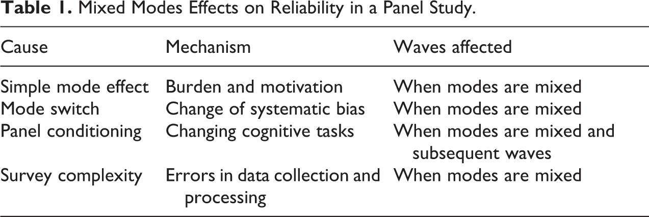
Considering the present theoretical framework, the reliability of the data in longitudinal studies can be influenced by four distinct factors. The first one is driven by the fact that cheaper modes are usually used in the mixed-mode design. The mechanism is the direct effect of collecting data in an alternative mode that increases the respondent burden and decreases motivation. An example of this is CATI, which uses only the auditory communication channel, thus increasing the burden on the respondent (De Leeuw 2005). Telephone interviews are also on average shorter compared to CAPI (e.g., Holbrook, Green, and Krosnick 2003), thus causing further cognitive burden. In addition, the distance to the interviewer, both physical and social, means that the respondent is less invested in the completion of the questionnaire, thus leading to lower quality data and more drop-offs. All these effects can lead to the increase of mistakes when responding to questionnaires using CATI and, therefore, to different degrees of reliability across modes.
The second mechanism is through the different systematic errors specific to each mode. In order to illustrate the process, I use recency (e.g., McClendon 1991; the tendency to select the last category) and primacy (e.g., Krosnick and Alwin 1987; tendency to select the first category) response styles as examples. We know that we can expect higher degrees of primacy in visual modes, such as CAPI with show cards, while recency is stronger in the modes that use only the auditory channel, such as CATI (Groves and Kahn 1979; Holbrook et al. 2007; McClendon 1991). If the mode-specific effects are stable in time, then models that estimate reliability, such as the quasi-simplex models, would overestimate reliability by including the systematic bias in the true score. Switching the mode, and changing the response style that is linked with it, leads to the movement of the variance due to the response style from the true score to the random error part of the model (i.e., the disturbance of the true score). Therefore, in the wave when the mode is switched, we expect lower reliability as the mode-specific systematic error is separated from the true score. This is true for all response styles that are mode-specific and stable in time. This is also true for all the systematic mode-specific effects caused by satisficing (Krosnick 1991; Krosnick, Narayan, and Smith 1996). In this framework, respondents who have lost the motivation to complete the questionnaire in an optimized way will choose to bypass some of the mental steps needed in the response process. Satisficing can be either weak, such as selection of first category or acquiescence, or strong, like social desirability or the random coin flip (Krosnick 1991). Thus, if the modes lead to a stable satisficing process, then we would expect a decrease in reliability proportional with the size of the mode-specific response bias and the proportion of the sample that responds using the new mode.
The third mechanism through which reliability can be influenced by mixing modes in longitudinal studies is panel conditioning. This is the process through which subjects change their responses because of the exposure to repeated measurements in time. This results in increased reliability and stability of items and decrease in item nonresponse (e.g., Chang and Krosnick 2009; Jagodzinski, Kuhnel, and Schmidt 1987; Sturgis, Allum, and Brunton-Smith 2009). Therefore, changing the mode of interview may lead to the decrease in this effect if the mode change leads to the practice of a different cognitive task. If this is true, then the reliability for the mixed-mode design should be smaller in subsequent waves (Dillman 2009).
The last factor leading to lower reliability in a mixed-mode design is the overall increase of the survey complexity. This, in turn, can lead to an increase in errors both during the fieldwork and during the processing of the data. If this is true, then we would expect differences in reliability between the two mode designs especially in the waves when we have multiple modes and less so in subsequent waves. Table 1 summarizes the possible effects of mixing modes on reliability in panel data compared to a single-mode design.
Mixed Modes Effects on Reliability in a Panel Study.
So far, relatively few studies have concentrated on quality indicators like reliability or validity in the mixed-modes literature (e.g., Jäckle, Roberts, and Lynn 2006; Chang and Krosnick 2009; Révilla 2010, 2012; Vannieuwenhuyze and Révilla 2013). For example, Révilla (2010) has found small mean differences in the reliabilities of items measuring dimensions such as political trust, social trust, or satisfaction using a multitrait-multimethod design. The highest difference was found between a CATI and computer-assisted Web interview mode in the political trust model. Unfortunately, these results are confounded with selection effects. A similar approach was applied using an instrumental variable that aimed to bypass this issue (Vannieuwenhuyze and Révilla 2013). Although some methodological limitations remain, initial results show small to medium measurement effects and relatively large selection effects. This article will contribute to this literature by adding a new analytical model that takes advantage of the longitudinal data and offers an estimation of reliability.
Reliability in Panel Data
In order to evaluate the effect of the mixed-mode design on the data quality, I concentrate on evaluating the impact on reliability. Using CTT, we can define the reliability as the percentage of variance of the observed variable that is due to the true score as opposed to variance caused by random error (Lord and Novick 1968). There are a number of models that aim to separate random measurement and true scores such as multitrait-multimethod (Campbell and Fiske 1959), confirmatory factor analysis (CFA; Bollen 1989), or the QMSM (Alwin 2007; Heise 1969; Wiley and Wiley 1970).
Considering the characteristics of our data, four waves of panel data, I concentrate on the strand of literature that tries to explain reliability using repeated measures as opposed to multiple items (Alwin 2007). A first attempt of assessing reliability using these kinds of measures was made by Lord and Novick (1968) who highlighted that by using two parallel measures we could estimate reliability. This term refers to measures that have equal true scores and equal variances of the random errors. If this is true, then the correlation between the two measures is a correct estimation of reliability. But, as the authors themselves highlight (Lord and Novick 1968:134), this approach assumes the absence of memory, practice, fatigue, or change in true scores. Especially, the latter and the former make this estimation of reliability unfeasible for most social science applications.
In order to overcome the assumptions of the test–retest approach, a series of models that take into account the change in time of the true scores were put forward. They usually assume an autoregressive change in time where the true score Ti is influenced only by Ti − 1 and no other previous measures. As a result, these models need at least three waves to be identified. In addition, they still need to make the assumption of equal variance of random error in order to be estimated (van de Pol and Langeheine 1990; Wiley and Wiley 1970). On the other hand, they offer two important advantages (Alwin 2007:103). First, they are able to separate random error from the specific variance of the true score. Second, under certain conditions, they can rule out systematic error as long as it is not stable in time.
In the next subsections, I present two such models. Although they are conceptually similar, imposing comparable assumptions and leading to estimates of reliability, they are developed from distinct statistical traditions and for different types of variables. As a result, QMSM can be used for continuous and ordinal variables by considering the true score continuous, while the LMC model has been developed to deal with categorical variables and views the true scores as discrete.
QMSM
The QMSM is composed of two parts. The first one, the measurement component, is based on CTT and assumes that the observed score Ai
is caused by a true score, Ti
, and random measurement error,


In addition to the measurement part, the model includes a structural dimension that estimates the relationships between the true scores. As a result of the autoregressive (simplex) change in time of the true scores, we have the following equations:


where β i, i − 1 is the regression slope of Ti − 1 on Ti and di is the disturbance term. The former can be interpreted as stability in time of the true score while the latter can also be interpreted as the specific variance of the true score at each wave. The model can be seen in Figure 1.
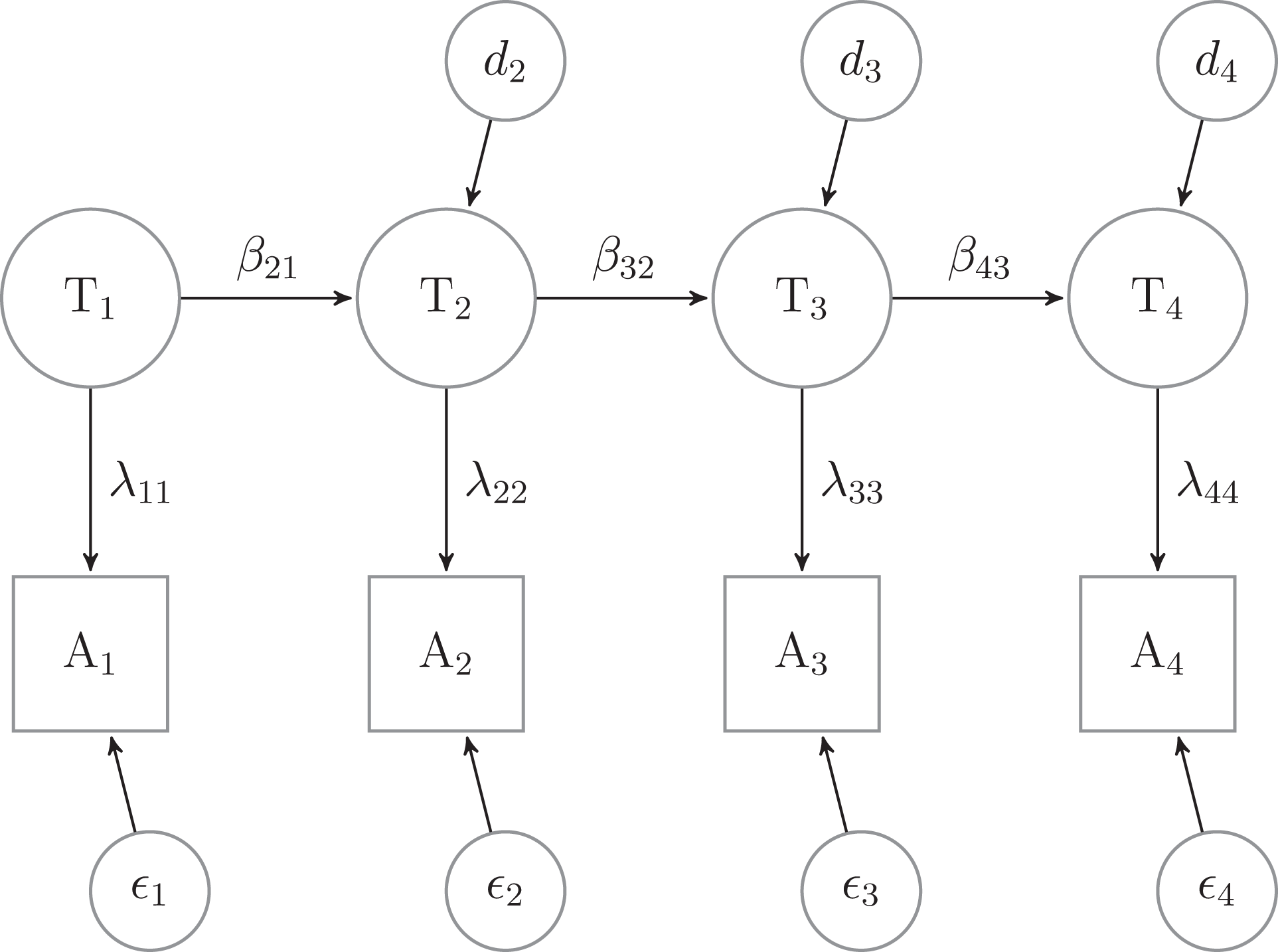
Quasi-Markov simplex model for four waves.
In order to identify the model, we need to make two assumptions. The first one constrains the unstandardized λ ii to be equal to 1:

In addition, I constrain the variance of the random errors, θ i , to be equal in time (Wiley and Wiley 1970)

Although the two assumptions have two different roles, they are both needed for identification purposes. The first one, equation (8), is necessary in order to give a scale to the latent variables (Bollen 1989) and is the standard practice in the CFA framework. The second assumption, equation (9), was proposed by Wiley and Wiley (1970) in their seminal article. The authors suggest that this assumption is sound theoretically, as the random error is a product of the measurement instrument and not of the population. And, albeit this assumption has been previously criticized (e.g., Alwin 2007:107), it is still less restrictive than that proposed by Heise (1969)—namely, that the reliability should be considered equal in time.
Given the previous equations and the definition of reliability in CTT, the percentage of variance explained by the true score (Lord and Novick 1968), I propose the following measures of reliability for each of the four waves: 1
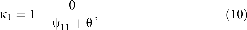
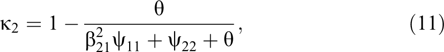
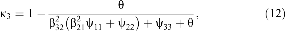

where
The QMSM has a series of assumptions that are needed in order to converge and give correct estimates of reliability and stability. In addition to those mentioned earlier, some of these include the following: The random errors and the time-specific true scores are not serially correlated, the random errors are not correlated with the true scores, and the true scores have a lag-1 time dependence.
LMC
Although the QMSM provides a reliability estimate for continuous and ordered variables, it cannot do so in the case of discrete, unordered, variables. In this case, a more appropriate model would need to take into account each cell of the variable. Such a model was applied to reliability analyses in panel data by Clogg and Manning (1996) and can be considered a LMC model based on the Langeheine and van de Pol (2009) typology. For simplicity, I consider all variables to be dichotomous, although the model can be easily extended to variables with more categories. I also assume that the true score has the same number of categories as the observed one, this being a typical approach to these types of models (Clogg and Manning 1996; Langeheine and van de Pol 2009; van de Pol and Langeheine 1990).
Let i, j, k, and l be the levels of a dichotomous variable A measured at four points in time: A
1, A
2, A
3, and A
4. By levels, I refer to the observed response to the item (e.g., answering “yes” may be level 1 and “no” may be level 2). The cell probability (ijkl) is denoted by
This notation can be included in an autoregressive model (i.e., quasi-simplex) with four latent variables:
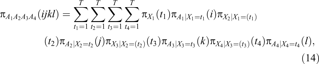
where X
1 − X
4 are the true scores at the four time points,
The reliability in this context can be calculated using the conditional odds ratio between Xi and Ai :
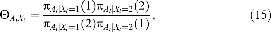
where
This can be transformed using Yule’s Q into a measure of association similar to R 2 (i.e., it is a proportional reduction in error; Alwin 2007; Clogg and Manning 1996; Coenders and Saris 2000):

Thus,
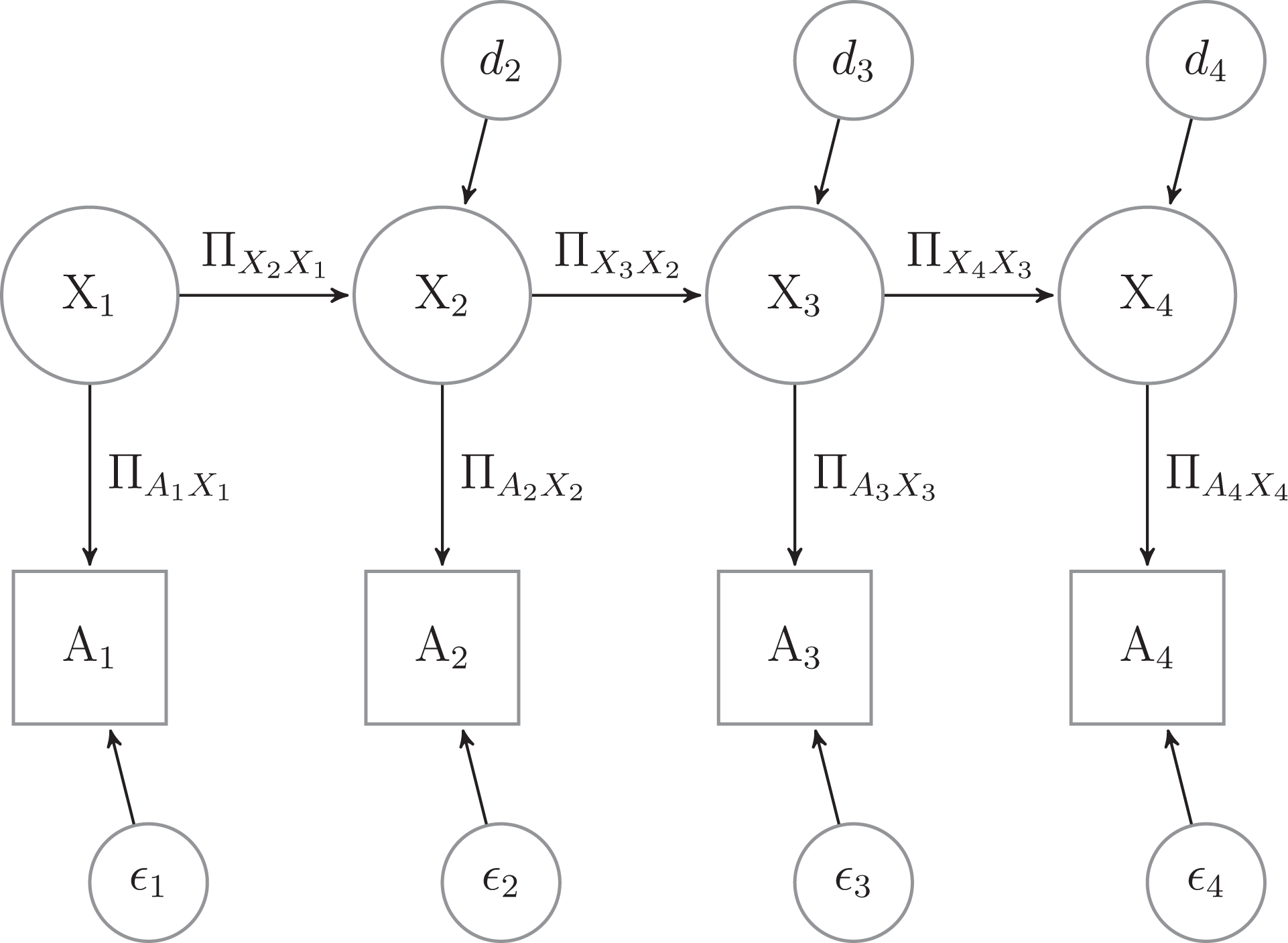
Latent Markov chain with four waves.
In order to identify these models, two important constraints are needed. The first one is time-homogeneity of latent transition probabilities (Alwin 2007; van de Pol and Langeheine 1990):

where

These assumptions imply that, unlike the QMSM, we can only have one estimate of reliability and one of stability 2 for each variable when using LMC. And, even if the two models give similar estimates of reliability, the assumption of equal reliabilities in time of LCM, equation (18), is conceptually different from the assumption of equal error variance in time of the QMSM, equation (9). As a result, the reliabilities of the two types of models will not be compared.
One possible risk of the LMC approach is the resulting high value of the reliabilities. Alwin (2007) highlights that in this kind of model, reliability is also a result of the number of categories of the observed variable. Therefore, in the case of items with two categories, high levels of reliability are expected. This is not a limitation of the method, as long as it can discriminate the mode design effect on reliability and stability.
Concluding the presentation of the two analytical approaches, I would also like to highlight that despite the similarity between QMSM and LMC, both conceptually and in one of the assumptions, they are two distinct approaches that come from different statistical traditions (Alwin 2007). In this article, I see this as an advantage, as it gives us two different ways of identifying the impact of mixing modes on measurement.
Furthermore, although I believe that reliability is an important quality indicator, it also needs to be highlighted that the models used here ignore the part of the variance that is systematic bias. Although a considerable part of the mixed-mode literature talks about types of systematic errors that manifest differently between modes, such as primacy/recency or social desirability (see Betts and Lound 2010; Dex and Gumy 2011; Roberts 2007, for an overview), the two models used here, QMSM and LMC, ignore the bias as long as it is stable in time. Thus, part of the mode-specific systematic bias is transferred to d 2. Keeping this limitation in mind, I propose three hypotheses.
Hypotheses
As motivated in The Impact of Mixing Modes and Reliability subsection, there are four main reasons why mixing modes would lead to a decrease in reliability in the respective wave. First, using a mode that leads to an increase in burden and a decrease in motivation for the respondent will lead to more mistakes and inconsistencies. Furthermore, as long as a mode-specific systematic bias exists, the change of mode for a part of the sample will lead to a decrease in reliability by moving this part of variance from the true score into the time-specific disturbance term. Third, changing modes can have an impact on panel conditioning, thus decreasing reliability and stability. Finally, the overall increase in complexity of data collection and processing due to the mixed-mode design will lead to the addition of random errors.
I also expect a decrease in stability when the mode switches in the mixed-mode design. This can be caused by the move of the mode-specific variance to either random error or to time specific true score. Thus, for the mixed-mode design, I expect lower stabilities from wave 1 to wave 2, when some respondents change from CAPI to CATI, and from wave 2 to wave 3, when the same respondents move from CATI to CAPI.
Additional impact of mixing modes on reliability is possible in subsequent waves. This effect is important for longitudinal studies, as it threatens comparability with previous waves even if the mode switch is temporary. One possible mechanism through which this may take place is panel conditioning. The change of mode can lead to a different type of cognitive task which, in turn, may stop the increase of reliability in subsequent waves.
Method
Data
The USIP is a yearly panel study that started in 2008 and is financed by the U.K. Economic and Social Research Council (Understanding Society: Innovation Panel, Waves 1-4, 2008-2011). The survey is used for methodological experiments. It uses a stratified and geographically clustered sample in order to represent England, Scotland, and Wales. Using the Postcode Address File, it applied systematic random sampling after stratifying for the density of the manual and nonmanual occupations in order to select 120 sectors. Within each of these sectors, 23 addresses were selected. The total number of selected addresses was 2,760. In wave 4, a refreshment sample of 960 household was added, consisting of an additional 8 addresses in each of the 120 sectors. Throughout the survey, all residents over age 16 were interviewed using CAPI. In this analysis, I will be using waves 1–4, which have been collected between 2008 and 2011. Wave 1 had an initial household-level response rate of 59.5 percent followed by household response rates conditional on previous wave participation (plus noncontacts and soft refusals in the previous wave) of 72.7 percent, 66.7 percent, and 69.9 percent, respectively, for subsequent waves (McFall et al. 2013). The household response rate for the wave 4 refreshment sample was 54.8 percent (McFall et al. 2013). The individual sample size for the full interview varies from a maximum of 2,384 in wave 1 to a minimum of 1,621 in wave 3.
One of the characteristics that was manipulated in the experiments of the USIP is the mode design. For example, in wave 2 of the survey, a CATI-CAPI sequential mixed-mode design was implemented for two-thirds of the sample and a CAPI single-mode design was used for a third. Furthermore, the sequential design was equally divided in a “telephone light” group and a “telephone intensive” group. In the case of the former, if one individual from the household refused or was unable/unwilling to participate over the telephone, the entire family was transferred to a CAPI interview while in the latter group such a transfer was made only after trying to interview all adults from the household using CATI (Burton, Laurie, and Uhrig 2010). Although this design decision is interesting, I consider the two CATI approaches together and refer to them as the CATI-CAPI mixed-mode design as opposed to the CAPI single-mode design.
Because the allocation to the mode design was randomized, we can consider the resulting data as having a quasi-experimental design. Using the notation introduced by Campbell and Stanley (1963), I can represent the data as seen in Table 2. The two groups have similar mode design (i.e., observations and are noted as O in the table) with the exception of wave 2, when the CATI-CAPI sequential design was introduced for a portion of the sample (highlighted by X in the table). In addition, the two groups are randomized (highlighted in the table by the use of R in the first column), as a result they should be comparable and all differences between them should be caused by the mode design.
Quasi-experimental Design of Mixed Modes in USIP.

Note: USIP = Understanding Society Innovation Panel; CAPI = computer-assisted personal interview; CATI = computer-assisted telephone interview.
In order to evaluate the impact of the mixed-mode design on the reliability of the items, I have selected all the items that were measured in the USIP in all four waves. A Stata.ado file that automatically evaluates the names of the variables in all four waves was used. Additional rules for selecting variables were applied. As a result, all variables that had less than 100 cases for each wave on the pooled data were eliminated. Variables that are not the direct results of data collection (e.g., weighting) or variables without variance (i.e., one category with 100 percent) were also eliminated.
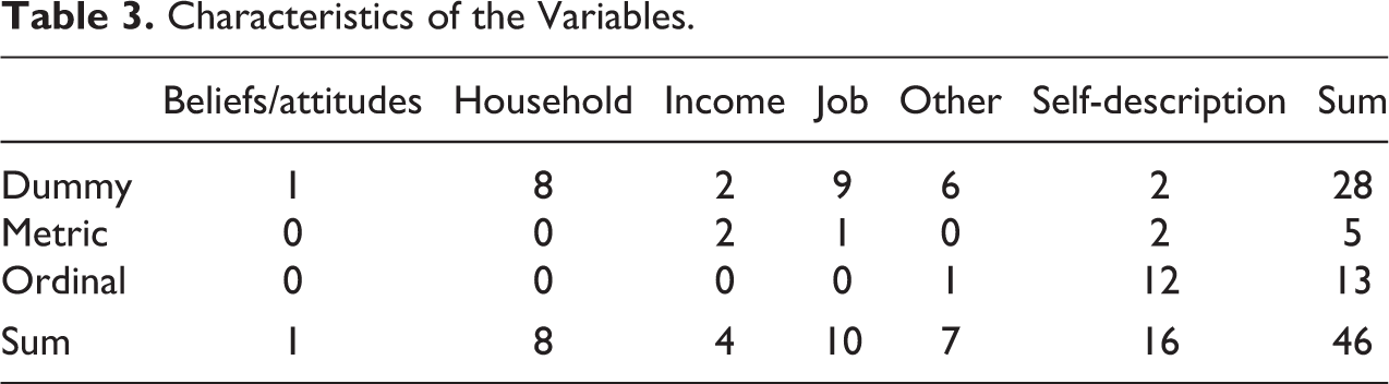
After this selection and the elimination of nominal variables, 3 a total of 46 variables remained. Of these 18 are analyzed using QMSM and 28 dummy variables using LCM. And while the dummy variables cover a wider range of topics, from beliefs and self-description to income and job, the metric and ordinal variables are concentrated on certain themes. The ordinal variables are mainly composed of the SF12, a health scale that measures both physical and psychological well-being (Ware et al. 2007). The continuous variables, on the other hand, measure total income, net and gross, self-description, namely height and weight, and the number of hours worked in a typical week. Each of these 46 variables will be analyzed using one of the two methods presented earlier in order to estimate differences in reliability and stability between the two mode designs (Table 3). 4
Characteristics of the Variables.
The data management and part of the analyses were made using Stata 12. The bulk of the analyses were done using Mplus 7 and the runmplus.ado.
Analytical Approach
For both types of analytical approaches, I used Bayesian Information Criterion (BIC) to compare the different models:

where k is the number of free parameters to be used and n is the sample size. This information criterion controls for both sample size and model complexity. Moreover, it does not assume the models are nested and it can be used consistently both for the QMSM and for the LMC. With this measure, a smaller value represents an improvement in model fit, as it minimizes the log likelihood.
Before exploring more the ways in which mode influence measurement, I need to highlight an important caveat. Although theoretically it makes sense to distinguish between measurement and selection effects in mode differences, these are harder to distinguish empirically. A small number of articles have tried to do this so far (Lugtig et al. 2011; Schouten et al. 2013; Vannieuwenhuyze and Loosveldt 2012; Vannieuwenhuyze, Loosveldt, and Molenberghs 2010). Usually, they do so either through a very complex survey design (e.g., Schouten et al. 2013) or by using a number of assumptions (e.g., Lugtig et al. 2011; Vannieuwenhuyze and Loosveldt 2012). In order to simplify the analyses, I will not distinguish between measurement and selection effects. Using the random allocation to mode, the total effect of the mixed-mode design can be estimated. As a result, differences between the two mode designs in reliability can be seen as a total effect that includes selection, measurement, and their interaction.
QMSM
The QMSM will be analyzed in a sequential order from the most general, less restricted, to the most constrained model. The first model (model 1) assumes that the unstandardized loadings are equal to one, equation (8), and that random measurement error is equal in time, equation (9), within mode design. Thus, nothing is constrained equal across the two mode designs. The next four models stem from the definitions of the reliabilities for the four time points. As a result, model 2 assumes that the variance of the true score in wave 1 (ψ11) and the variance of the random error (θ) are equal across designs. If this is true, then the reliability for wave 1 (
Although QMSM represents one of the best models we have for measuring reliability with repeated items, it is marred with estimation issues. Two of these are the negative variances and standardized stability coefficients over 1.0 (Jagodzinski and Kuhnel 1987; Van der Veld and Saris 2003). While Coenders et al. (1999) and Jagodzinski and Kuhenl (1987) explore the causes of these issues, I propose a possible solution here. Instead of estimating the models using maximum likelihood methods, I employ Bayesian estimation. This has the advantage that it needs smaller sample sizes and does not result in unacceptable coefficients (Congdon 2006). Although these advantages are important, the Bayesian estimation has two drawbacks: It cannot use weights and multigroup comparisons have not yet been implemented in the software used. The latter is especially important, as I aim to compare the two mode designs. In order to bypass this issue, I have taken advantage of the fact that this estimation algorithm can deal with missing data using the Full Information procedure (Enders 2010; Muthén and Muthén 2012). Using this approach, all the information in the data is used for the analysis. We can take advantage of this and model two parallel QMSM for the two groups, although there are no common cases, by imposing the lack of any relationship between them. 5 I will be using the Bayesian implementation in Mplus 7 with the following parameters: four chains, thinning coefficient of five, convergence criteria of 0.01, and a maximum of 70,000 iterations and a minimum of 30,000 (Muthén and Muthén 2012).
LMC
The estimation procedure for LMC will include three distinct models. These start once again from the least restrictive and progresses to the most restrictive model. As a result, model 1 will assume that both the transition probabilities in time and the reliabilities are equal in time within mode design, equations (17) and (18). Model 2 imposes the additional restriction that the reliability is the same for the two mode designs (i.e.,
By comparing the three models using the BIC, we are able to see which model fits the data best. If model 1 is the best fitting one, then we conclude that both the reliabilities and the transition probabilities from one wave to another (i.e., stabilities) are different across modes. On the other hand, if model 3 is the best fitting one, then we can assume that both the reliability and the stability are equal across the two mode designs. If model 2 is the best fitting one, then we can assume that the reliabilities are equal but the stability of the true scores is not.
In order to estimate the model, I use Robust Maximum Likelihood estimation with 500 maximum number of iterations and random starts: 200 initial stage random starts and 20 final stage optimizations. In order to be consistent, I use no weights but the Full Information procedure will be applied.
Analysis and Results
Previous research has highlighted that the QMSM is an unstable model and can sometimes either not converge or give out of bounds coefficients (e.g., Jagodzinski and Kuhnel 1987; Van der Veld and Saris 2003). Although using the Bayesian approach bypassed most of these issues, 6 it did prove problematic for three of the continuous variables, two items measuring income and one measuring weight. While the models converged when analyzed by mode design, our parallel quasi-simplex chains approach did not lead to convergence even when increasing the maximum number of iterations or the thinning coefficient. As a result, I could compare the reliabilities and stabilities across modes for these variables but I would not be able to use the same approach as presented in the QMSM subsection under Methodology section. Consequently, these three variables will be ignored in the following analyses. Similar issues have arisen in the case of LMC. Of the initial 28 items, 10 have issues in convergence, involving either a nonpositive definite first-order derivative product matrix or a nonpositive definite Fisher information matrix. One of the solutions proposed, increasing the number of random starts, did not prove successful in any of the models. The items were concentrated on two main topics. Four of them were measuring attributes linked with the household and were derived from household-level information. Four of the items were measuring job and income-related aspects, such as whether the respondents are full-time or part-time employed. These 10 variables will also be ignored in the following analyses. Therefore, our actual variable sample size is 33, 13 being ordinal variables, 2 continuous, and 18 dichotomous.
The sample sizes of the analyses are moderately high because of the Full Information procedure. Thus, for QMSM, the median is 1,790 and the minimum 1,020. On the other hand, the sample sizes are somewhat smaller for the LMC, reaching 534 cases for a variable measuring if the respondent is living in the household with the partner, but still with a median of 1,775 individuals included per analysis.
QMSM
Concentrating on the 15 ordered variables, 12 of them measure health-related aspects while the other 3 measure height, number of work hours, and when they last weighed themselves. Each of these items was analyzed five times, each time imposing a new constraint, as presented in the QMSM subsection under Methodology section. This procedure results in 75 models. Within each variable, I compared the BIC of the five models. A decrease in this coefficient indicating an improvement in the model fit while controlling for sample size and model complexity.
Looking at the mean goodness of fit of the models as constraints are added, I observe that moving from model 1 to model 2 leads to a mean decrease in BIC of 33. Similar results are found by adding the constraints of model 3. Adding the mode equality of model 5 to model 4 leads to a further mean BIC improvement of 27. Overall, each constraint leads to improvement of fit and usually model 5 proves to be the best fitting one. This implies that there is no difference between the two mode designs in reliability or stability for the ordered variables.
Table 4 presents the exceptions to the linear decrease in BIC with the additional constraints. If we look in the sequence of models for the best fitting one and consider that as the best representation of the data, then Height is the only variable that does not have model 5 as the best fitting model. In this case, model 2 appears to be the most appropriate representation of the data. Therefore, in the case of Height, either the reliability or the stability to wave 2 is different between the two mode designs. Looking in more detail at the estimates of model 2 for height, we observe that although reliabilities are very similar, 0.974 for the single-mode design versus 0.976 for the mixed mode, the difference in the stability 7 of the true score from wave 1 to wave 2 is bigger, being 0.966 for the former and 0.997 for the latter. Therefore, it appears that the stability of the Height variable from wave 1 to wave 2 is significantly higher in the CATI-CAPI mixed-mode design than in the CAPI design.
BIC Differences within Variables.
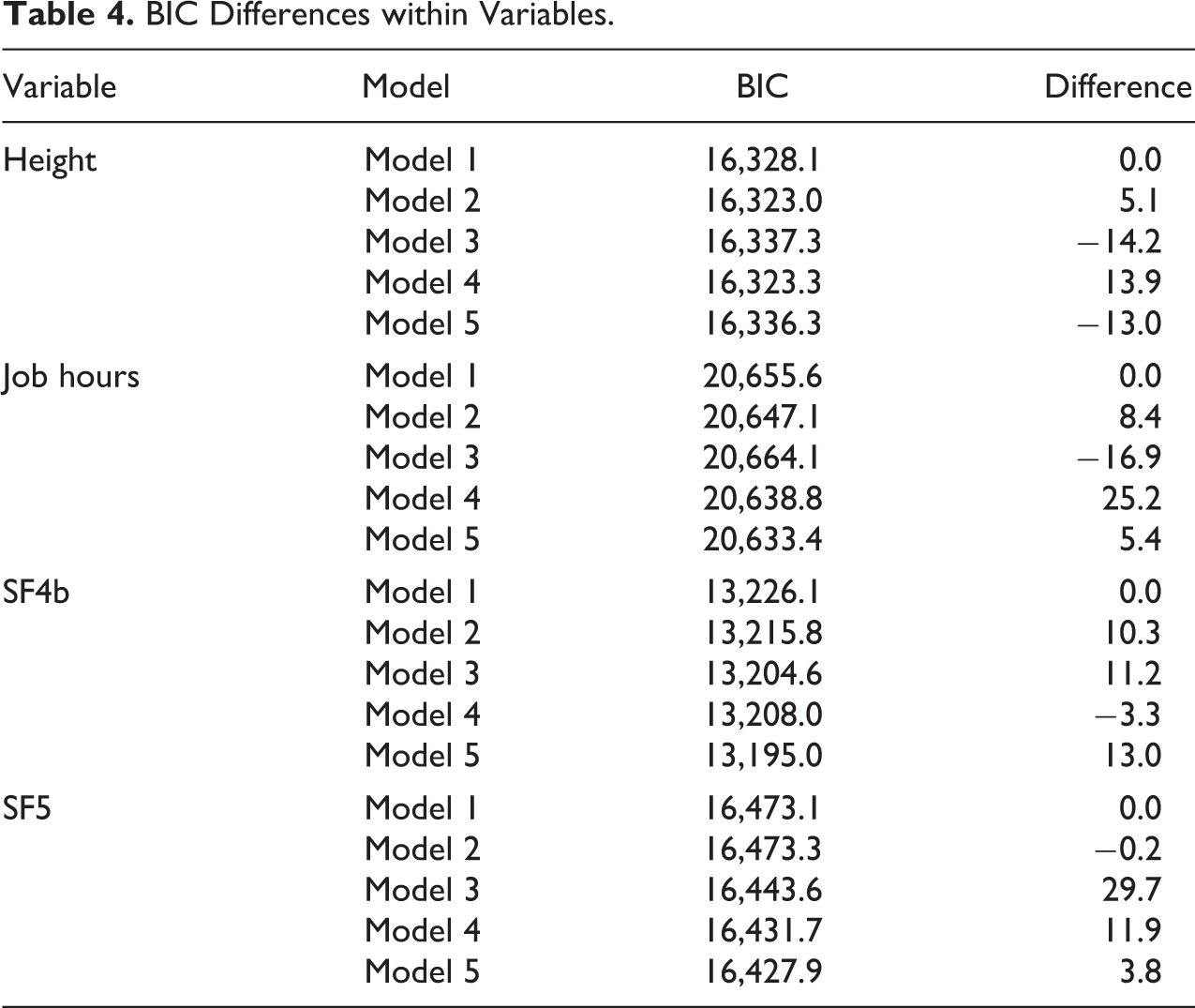
A somewhat similar pattern is indicated by the other three variables presented in Table 4, although they point to model 5 as the best fitting model. For example, in the case of model 2 for Job hours, we see that even if the single-mode design shows somewhat larger reliability for wave 2, 0.931 versus 0.924, the stability from wave 1 to wave 2 for the mixed-mode design is considerably higher, 0.867 versus 0.726. Similarly, in the case of model 3 of SF4b, reliability in wave 3 is higher for the CAPI design, 0.566 as opposed to 0.445, but the stability from wave 2 to wave 3 is lower, 0.580 versus 0.940. Similar results can be seen for SF5 for wave 1 in model 1, although with smaller differences (Figure 3).
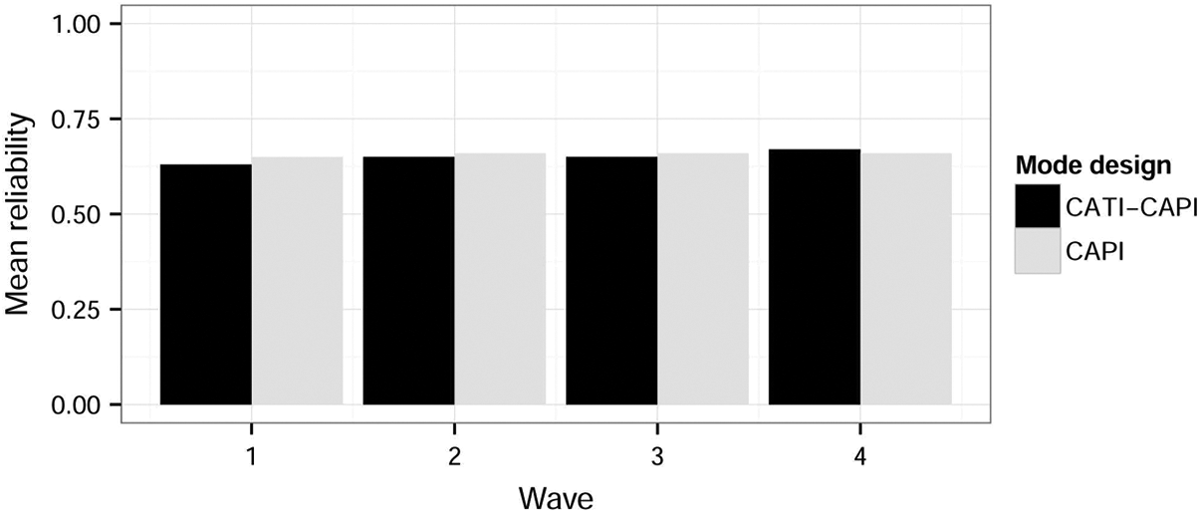
Mean reliability ordered variables (model 1).
Looking at the overall reliability patterns, we observe very small differences between the groups with a moderate mean level of reliability for all the ordered items analyzed. Additionally, Figure 4 shows the change over time in the mean stability of the items. Here, we also find very small differences between the groups, with an overall increase of stability in time. This is an expected result and can be explained in terms of both panel conditioning (Sturgis et al. 2009) and as a selection in time of “good” respondents (Brehm 1993). Running the same analyses on a balanced panel led to similar increase in stability over time. This provides an argument for panel conditioning as opposed to selection.
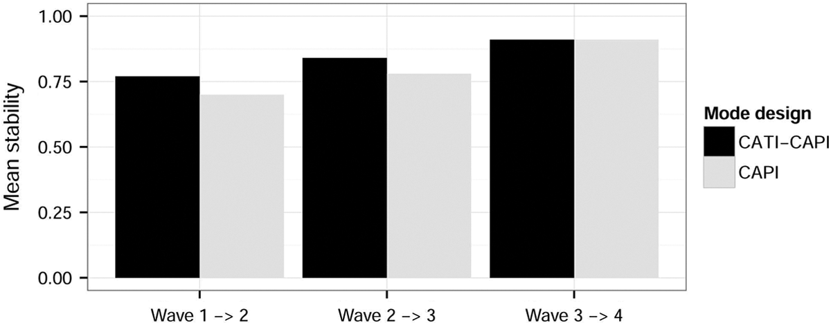
Mean stability ordered variables (model 1).
LMC
In addition to the QMSM, I have analyzed 18 dichotomous variables. For each of these, I estimated three models, as presented in the LMC subsection, resulting in 54 models. Overall, similar results have been found. On average, the constraints of model 2, equal reliabilities in time, bring a mean improvement in BIC of 18. A similar result appears when the additional constraint of equal stability across modes designs is imposed. The linear improvement of fit with the two additional constraints is true for all the variables analyzed.
Looking at the mean reliabilities and stabilities, we find similar results as in the case of QMSM. The models indicate high reliabilities that are consistent across the two mode designs. For both of them, the mean reliability is 0.98. A similar conclusion can be reached in the case of stability. On average, the mixed-mode group had a stability of 7.4 while the one for the single-mode design was 9.5 on a log odds scale. These high levels of stability indicate that there is little time-specific change in true score for the variables measured here. This may be caused by a number of factors, two of the most important ones being the fact that change is dependent on the number of categories of the variables (i.e., fewer categories imply smaller probability of change) and that the variables analyzed here may have small degrees of change in time. As the BIC results indicate, the differences between the two mode designs in stability and reliability do not withstand.
Conclusions and Discussion
The Impact of Mixing Modes and Reliability subsection argued that mixing modes will have a detrimental impact on reliability, especially when one of the modes brought additional respondent burden and lead to a decrease in motivation. The results of our analyses do not confirm this hypothesis. In the case of QMSM, I have found only 1 of the 15 variables that did not indicate model 5 as the best fitting one. A similar result was found when using LMC. Here, model 3 was always the best fitting one, indicating once again that stability and reliability are equal between mode designs. This implies that for almost all the variables analyzed here, the reliability and stabilities were equal across modes.
By using the QMSM, I was also able to analyze the impact of mixing modes on subsequent waves with regard to reliability. I have argued in The Impact of Mixing Modes and Reliability subsection that mixing modes may lead to a decrease (or lack of increase) in reliability compared to a single-mode design. One potential explanation for such an effect is panel conditioning, the mixing of modes leading to a different type of cognitive task that, in turn, would decrease the impact of training. Our results do not support this hypothesis. No differences in reliabilities between the two mode designs in waves 3 and 4 are observed. The result of no differences across mode designs regarding panel conditioning is the first one of its kind, to the knowledge of the author, and may indicate that at least on this dimension, longitudinal reliability, and for these types of variables panel studies are “safe” from mixed-mode specific effects.
Furthermore, Hypothesis 2 has also been rejected by the data. A decrease in stabilities was expected because some of the respondents changed the modes used. The two mode switches implied by the mixed-mode design, from CAPI to CATI (wave 1 to wave 2) and from CATI to CAPI (wave 2 to wave 3), did not have a significant impact on the stability of the true score. This can be either due to the lack of differences between the two groups or because the model already takes into account the random error characteristic to each mode design.
Looking in more detail at the panel conditioning, I have found mixed results. The finding of constant reliability in time is an unexpected one, as previous research has shown effects of panel conditioning (e.g., Jagodzinski et al. 1987; Sturgis et al. 2009). Although an effect of panel conditioning on reliability was not present, there was one on stability. Thus, stability of the true scores increases in time even if no mode differences are apparent. Because similar results were found when a balanced panel was analyzed conditioning appears more plausible than selection.
Although the overall results in the QMSM indicate that reliability and stability are similar across the two mode designs, there are a few exceptions worth mentioning. First, only one variable did not indicate model 5 as the best fitting one. In this case, the higher stability in the mixed-mode design seems to be the main driver. Similarly, three other variables did not show linear improvement of fit although model 5 still was the best fitting one. In these cases, a pattern of higher reliability for the single-mode design versus higher stability for the mixed-mode design appeared. This is an unexpected result and further research is needed in order to see if this is a substantially important result or an artifact of the statistical modeling.
Although the results are not definitive and further replications are needed, these results indicate that reliability may not be the main threat to cross mode designs comparisons. If these results are replicated, then selection (Lynn and Kaminska 2013; Vannieuwenhuyze and Révilla 2013) and response styles (e.g., Jäckle et al. 2006) may prove to be more important issues than reliability. Although the analyses show that random error is the same in the two mixed-mode designs, the same cannot be claimed about systematic error that is stable in time (e.g., Billiet and Davidov 2008). In order to capture this variance, alternative approaches are needed, such as multitrait-multimethod (Saris, Satorra, and Coenders 2004) or modeling of response styles (Billiet and Davidov 2008; Billiet and McClendon 2000).
The study has also contributed to the methodological field by proposing two important solutions to some of the estimation issues that have marred QMSM (Jagodzinski and Kuhnel 1987; Van der Veld and Saris 2003). First, I have proposed Bayesian estimation as a way to avoid out of bounds coefficients. This has proved successful, as all the models that used this approach converged with coefficients inside the theoretical limits. In addition, a solution to the lack of multigroup modeling when using this estimation method has been proposed. Taking advantage of the Full Information method used for missing data, I have modeled two parallel quasi-simplex chains and constrained all covariances between them to zero. This has proved successful for all but three items. Although these have converged when analyzed by mode, they did not when using this method. More research is needed to understand exactly why this happened.
A series of limitations of the study also need to be highlighted. First, I do not make the distinction between selection and measurement effects but talk about the total effect of mixing modes. Using the random allocation to the design, I am able to show the total effects of mixing modes. These results are correct as long as the measurement and selection effects do not impact reliability in opposite directions. Furthermore, I cannot say anything about the decomposition into measurement and selection effects.
Another limitation refers to the modeling approach used here. The QMSM modeling may result in the overestimation of reliability if response styles are stable over time. Previous research has indicated that this may be the true in some cases. For example, Billiet and Davidov (2008) show that the acquiescence factor modeled using two balanced sets of items tapping Distrust in Politics and Perceived Ethnic Threat is stable over time. If this is true for response styles that affect the items tested here, then the QMSM may provide overestimated reliability coefficients. Although this may be an important threat in normal analytical designs, it should be highlighted that our conclusions are biased only if the response-style stability is different for the two mode designs.
Additionally, our results are also confounded with the different attrition patterns created by the mixed-mode design in wave 2. Previous results have shown that the two mode designs lead to different response rates and some minor differences in attrition patterns and response bias (Lynn 2013). Although the Full Information method assumes Missing At Random, this is true only if the missing mechanism is included in the model (Enders 2010). The models used here imply that the missing pattern respects a 1-lag Markov chain. If this is not true and the unexplained missing data are linked with reliability, then it will confound our results. In order to gauge the degree to which response rates and attrition may be issues, I have compared our results to those from using a balanced panel. No differences were apparent.
Another potential limitation of the study may be the high levels of reliability and stability in LMC. These bring doubts regarding its usefulness as an instrument for measuring data quality for dichotomous variables. Even if it is very attractive due to the lack of distributional assumptions, it may also prove not sensitive enough to find differences across groups, especially where big discrepancies are not obvious. Nevertheless, the model has been previously able to find heterogeneity between groups (e.g., van de Pol and Langeheine 1990) and the results found here may only be caused by the small differences across the variables compared (Clogg and Manning 1996; Langeheine and van de Pol 2009). This last argument being also supported by the general consistency of the LMC with the QMSM.
Finally, the analyses presented in this article did not take into account the different subgroups that may be more susceptible to these design changes. As such, possible extensions of this article can look in more detail at special subgroups, such as respondents with low cognitive abilities or language skills, or at more attitudinal and sensitive questions as these may prove to be more susceptible to mode design effects. Such development should also be encouraged for different types of mixed-mode designs and for different cultural backgrounds.
Footnotes
Acknowledgment
I would like to thank all the people who helped with this article: Peter Lynn, Nick Allum, Peter Lugtig, Noah Uhrig, and Jakob Peterson.
Declaration of Conflicting Interests
The author(s) declared no potential conflicts of interest with respect to the research, authorship, and/or publication of this article.
Funding
The author(s) disclosed receipt of the following financial support for the research, authorship, and/or publication of this article: This work has been supported by a +3 ESRC scholarship (PG124701).