
Abstract
This article examines the impact of homeownership on subjective well-being and how it varies by location, age and income in Australia. We apply panel data models with instrumental variables within a two-stage modelling framework and find that homeownership, particularly outright ownership, positively affects subjective well-being – as measured by life, financial, home and neighbourhood satisfaction – relative to renting. However, these effects are not homogeneous. Outright owners in major urban locations enjoy higher financial satisfaction but poorer neighbourhood satisfaction than their counterparts outside major urban locations. The subjective well-being gap between owners and renters widens as age increases within the age range of 30s to 60s. However, the presence of mortgage debt depresses the financial satisfaction associated with homeownership. Beyond age 50, the existence of a mortgage debt burden cancels any positive financial satisfaction effects that homeownership has relative to renting. As income increases, the positive effects of homeownership on subjective well-being diminishes in the domain of financial satisfaction This reflects greater diversification in high-income households’ asset portfolios compared to low-income households’ portfolios. We discuss the policy implications of these heterogeneous effects.
Introduction
This article examines the links between homeownership and subjective well-being (SWB) in Australia and whether these links are moderated by location, age and income. We therefore, estimate tenure effects across four SWB domains in the form of life, financial, home and neighbourhood satisfaction.
For Australians, homeownership is assumed to be a universal aspiration and is widely held as a social ideal reflecting adulthood, prosperity and individual liberties (Colic-Peisker et al., 2015). Given the perceived benefits of owner-occupation, it is traditionally expected that homeownership will improve overall life satisfaction (Rohe and Stegman, 1994). As noted by van Praag et al. (2003), life satisfaction is a composite of different SWB domains. Thus, homeownership may have heterogeneous effects across different SWB domains. For example, long-run increases in real housing prices and the growing financialisation of housing assets (Aalbers, 2016; Adkins et al., 2021) may boost the financial satisfaction of homeowners relative to renters with similar incomes (Manturuk et al., 2012). Also, the quality of owner-occupied dwellings is, on average, higher than that of rental dwellings (e.g. Boehm and Schlottmann, 2008; Elsinga and Hoekstra, 2005), which might generate higher satisfaction with the home. Homeownership is linked to stronger social capital (Bloze and Skak, 2015; Leviten-Reid and Matthew, 2018), which can boost neighbourhood satisfaction.
On a national scale, homeownership has become a cornerstone of economic and social policy. Residential property assets amounted to AU$7779 billion or two-thirds of total asset holdings in households’ balance sheets in 2020 (Australian Bureau of Statistics (ABS), 2021). The trade-off between homeownership and the welfare (Castles, 1998) is deeply entrenched in the design of the Australian retirement income system. Fiscal policy measures preference the accumulation of wealth in the owner-occupied home through generous tax-transfer concessions. Government age pensions have remained at low levels by international standards based on the assumption that low-income retirees can live on small pensions due to low housing costs associated with outright ownership in retirement. This significantly reduces after-housing cost poverty among older Australians (Yates and Bradbury, 2010). Due to the importance of housing asset-based welfare in retirement, homeownership is dubbed the fourth pillar of Australia’s retirement incomes system, the other three pillars being a publicly provided age pension, mandatory private superannuation saving and voluntary saving (Bradbury, 2013; Saunders et al., 2022).
This article makes an important policy contribution by presenting evidence on the benefits of homeownership through a well-being lens. In recent decades, there has been concern that financial metrics alone are insufficient indicators of policy success. The idea of SWB was popularised among economists like Easterlin, who published seminal work examining the relationship between income and happiness and found that a rise in average income does not necessarily lead to an increase in SWB (Easterlin, 1973, 1974). There is now growing acceptance that well-being is an important measure of whether citizens’ lives are improving due to policy interventions (OECD, 2019).
Within the literature, there exists a vast pool of studies on the links between tenure and SWB. However, the evidence base is heavily weighted towards studies focused on a binary own–rent divide, and assumes that the links between homeownership and SWB are homogenous, relying on a single SWB measure to derive conclusions. We expand the breadth and nuance of the existing evidence base in three ways. First, we distinguish across three tenures, that is, outright ownership, mortgaged ownership and renting. Second, we model the heterogeneity of the homeownership–SWB links across four SWB domains. Third, we uncover varying impacts of homeownership on SWB by location, age and income. We set out four hypotheses below.
Hypotheses
The existing literature generally agrees that a positive SWB gap exists between owners and renters; that is, owners’ SWB exceeds renters’ SWB. We extend the existing evidence base by testing four hypotheses in relation to this SWB gap.
H1: SWB is higher for owners than renters. However, among owners, SWB is higher for outright owners than mortgagors
The first hypothesis is underpinned by the phenomenon of growing mortgage debt burdens. As the cost of accessing homeownership has increased with soaring house prices, growing numbers of Australians now carry mortgage debt in later life. Our own calculations from the Australian Surveys of Income and Housing show that among homeowners aged 25–34 years old, the share holding a mortgage climbed from 79% to 96% between 1990 and 2017. Among homeowners aged 55–64 years, the share of mortgagors rose from 15% to 51%. Among mortgagors, loan-to-value ratios (LVRs) also rose across all age groups.
H2: The positive SWB gap between owners and renters is smaller outside major urban locations than within major urban locations
The second hypothesis relates to the trade-off between home purchase affordability and location. Young first homebuyers are increasingly pushed to the urban fringe to purchase where housing is more affordable (Burke et al., 2014). However, fringe suburbs are often plagued by poor access to essential services and job opportunities reflecting smaller population numbers.
H3: The positive SWB gap between owners and renters widens as age increases
Financial deregulation in recent years has prompted the growing use of in situ mortgage equity withdrawal that allows homeowners to draw down on their housing equity to fund spending needs. Existing studies show that this may be used to support spending needs associated with child-raising in mid-life, but is especially important in old age as a resource to fund health and aged care needs, and the home maintenance needed to support ageing in place (Ong et al., 2015). This resource is not available to renters.
H4: The positive SWB gap between owners and renters narrows as income increases
The asset portfolios of low-to-middle-income households tend to be dominated by housing wealth, while higher-income households’ portfolios are less reliant on housing (Skott, 2013). Thus, we expect the SWB benefits of homeownership to decline relative to renting as income increases.
Literature review
SWB is multi-faceted and can be measured in various ways (Clapham et al., 2018). Studies modelling links between housing and SWB mostly focus on questions around satisfaction (particularly in the field of economics) or self-assessed mental and physical health (particularly in social epidemiology). Given our study’s focus, we present a literature review on the links between housing tenure and satisfaction, typologising the review by each of the four satisfaction measures in the domains of life, financial, home and neighbourhood.
Among the four satisfaction measures, overall life satisfaction has been most widely investigated. Studies generally find a positive link between homeownership and life satisfaction. Examples include Hu (2013) and Zhang et al. (2018) in China, Rohe and Stegman (1994) and Rohe and Basolo (1997) in the USA, Ruprah (2010) in Latin America and Zumbro (2014) in Germany. In Europe, Angel and Gregory (2023) find that owner-occupiers have higher life satisfaction than private renters in the UK and Austria, despite the two countries having different welfare regimes and tenure structures. However, Odermatt and Stutzer’s (2022) recent study finds that homebuyers systematically overestimate the long-term life satisfaction gained from owner-occupation. Other studies highlight moderating effects. For instance, Zumbro (2014) found that the links between homeownership and life satisfaction are moderated by dwelling conditions. Other studies test for the moderating effects of gender, city, age and income by running their models in these subsamples but find little difference across the subsample groups (Hu, 2013; Zhang et al., 2018).
The literature also shows a positive link between homeownership and financial satisfaction, but there are some caveats. Manturuk et al. (2012) find that among low-income owners and renters experiencing similar financial hardship levels, the former are more financially satisfied. Tharp et al. (2020) show that in the USA, homeownership has a positive association with financial satisfaction, though this is partly offset by the presence of mortgage debt. Plagnol (2011) also find a positive effect between homeownership and financial satisfaction, but this effect is smaller than owning financial assets. André et al. (2019) focus on post-divorce SWB among Australians and find that the role of homeownership as a buffer for financial (and life) satisfaction after divorce is limited.
In regard to housing satisfaction, the literature heavily favours the proposition that homeownership leads to higher housing satisfaction than renting. See, for instance, Hu (2013) and Zhang et al. (2018) in China, and Diaz-Serrano (2009) and Elsinga and Hoekstra (2005) in the EU.
Studies on the associations between homeownership and neighbourhood satisfaction also typically unearth positive associations, including Brounen et al. (2012) in Rotterdam, Grinstein-Weiss et al. (2011) for low- and-moderate-income households in the USA, and Ma et al. (2018) in Beijing. However, some studies show that various factors moderate this positive link. Brounen et al. (2012), using data from the city of Rotterdam, show that the positive links between ownership and neighbourhood satisfaction are significantly moderated by neighbourhood safety. Greif (2015) found that because homeownership increases residents’ sensitivity to local area conditions, it enhances neighbourhood satisfaction in advantaged communities but depresses neighbourhood satisfaction in distressed communities in Los Angeles. Parkes et al. (2002) show that English homeowners’ neighbourhood satisfaction levels are reduced in areas with lower owner-occupier shares, reflecting concerns with poor social interaction.
The background literature is clearly extensive. However, a significant opportunity exists to enhance the nuance of the evidence base, which our study offers. First, the majority of studies are interested in the own–rent divide but ignore the divide between outright owners and mortgagors despite growing mortgage indebtedness in nations such as Australia. Examples include Diaz-Serrano (2009) in Europe; Greif (2015), Grinstein-Weiss et al. (2011) in the USA; Zhang et al. (2018) in China; and Zumbro (2014) in Germany. We distinguish across three tenures – outright owners, mortgagors and renters. Second, we extend the currently narrow evidence base that highlights the influence of moderators on the ownership–SWB link via interaction terms in econometric models. In a third contribution, we investigate SWB measures across multiple dimensions by exploring satisfaction with one’s life, finances, home and neighbourhood within one study. While most studies focus on one or two satisfaction domains, the breadth of our comparisons across the same sample will highlight the extent to which homeownership affects satisfaction in one domain but not another while holding the sample composition constant.
Methodology
Data and sample
The analysis draws from the 2002–2018 Household, Income and Labour Dynamics in Australia (HILDA) Survey, Australia’s only nationally representative longitudinal dataset. 1 The survey is particularly suited for this study as it contains a comprehensive range of information relating to respondents’ socio-demographic, income, wealth, housing characteristics, and health.
The main variables for our analysis are SWB, for which respondents are asked to answer their satisfaction in each of multiple domains on an ordinal scale of 0 (totally dissatisfied) to 10 (totally satisfied). Further discussion of the strengths and limitations of these satisfaction variables is presented in the Online Supplemental Section S1.
Another key variable is housing tenure. We pool person-periods from independent adult respondents aged 21 years and over who are either homeowners or private renters. For each person, waves in which they are in public housing, rent-free or in the parental home are excluded due to highly subsidised or negligible housing costs. Waves in which a single person is living with other unrelated singles in a group household are also excluded as their dwelling’s legal owner cannot be identified consistently. We also exclude a small number of waves in which a person lives in a mobile dwelling, for example, a tent or caravan. Filtering these observations allows us to classify housing tenure into three categories; renters, owners without a mortgage (outright owner), and owners with a mortgage (mortgagor).
Modelling strategy
The standard approach to modelling ordered categorical variables, such as HILDA’s satisfaction variables, is the ordered logit or ordered probit model. Both models postulate that the observed ordered categorical outcome
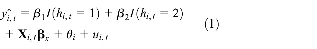
where
Equation (1) also includes the time-invariant individual-specific effect,
The ordered SWB outcome

where k = 0, …, 10 and
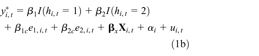
We consider two specifications of equation (1). The first is a ‘restricted’ model which specifies the coefficients of two binary tenure variables
where
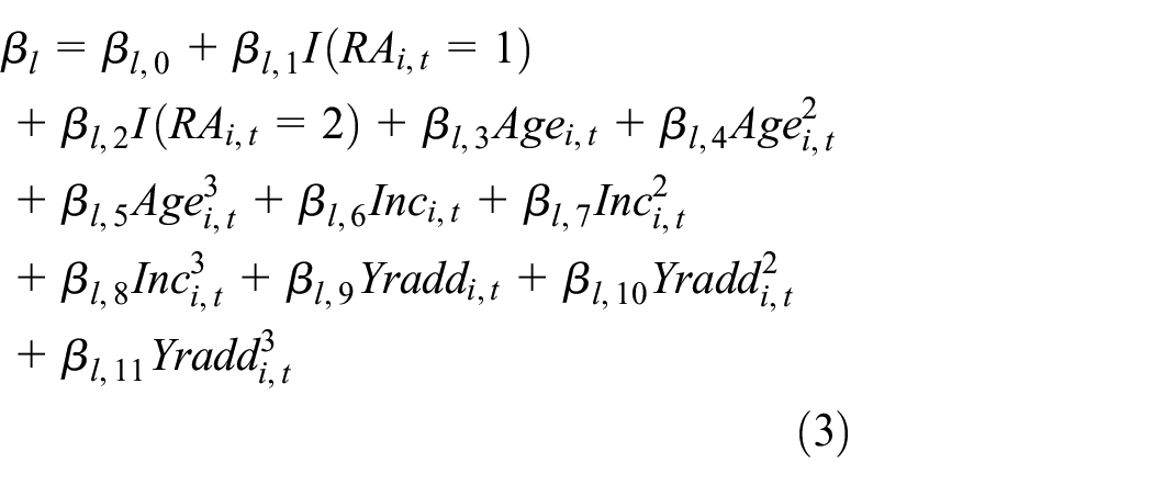
The effects of other covariates are specified as,
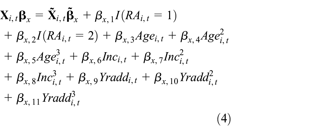
where
Hypothesis testing
We address H1 in two ways. First, we test the significance of the housing tenure coefficients,
Estimation issues
Estimation of model (1) is subject to two major econometric issues. The first is the endogeneity of the housing tenure variable,
To address the first issue, we apply the two-stage residual inclusion (2SRI) method (Terza et al., 2008), which yields a biased yet consistent estimate of the coefficients in model (1). Following this method, we first estimate an auxiliary model where the two endogenous housing tenure variables are regressed on a set of covariates and instrumental variables (IVs). An IV is an exogenous variable, that is correlated with the endogenous housing tenure variables but not with the idiosyncratic error on the right-hand side of (1).
We draw on IVs capturing receipt of parental transfers, the occupation of the respondent’s father when the respondent was growing up, and the user cost of homeowning. The first two variables reflect the respondent’s chances of receiving financial assistance from their parents with home purchase. Various studies have confirmed the importance of intergenerational transfers in assisting with home purchase (Helderman and Mulder, 2007; Köppe, 2018), yet they have no direct impacts on well-being (Ong et al., 2018). The user cost of homeowning is a key predictor of tenure choice. It captures the annual cost of owning a property expressed as a percentage of the house value. 5 It is also a key input into the relative cost of owning versus renting, which is widely used as an instrument for homeownership (Brounen et al., 2012; Manturuk et al., 2009).
The housing tenure variable takes three discrete values. Thus, we employ a multinomial logit model in the first stage of 2SRI. The model specifies the probability of individual i falling into category l (l = 1, 2) of housing tenure as,
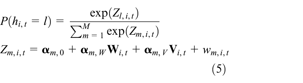
where
In the second stage, we calculate, for each of the two homeownership categories (l = 1 and 2), the predicted probability
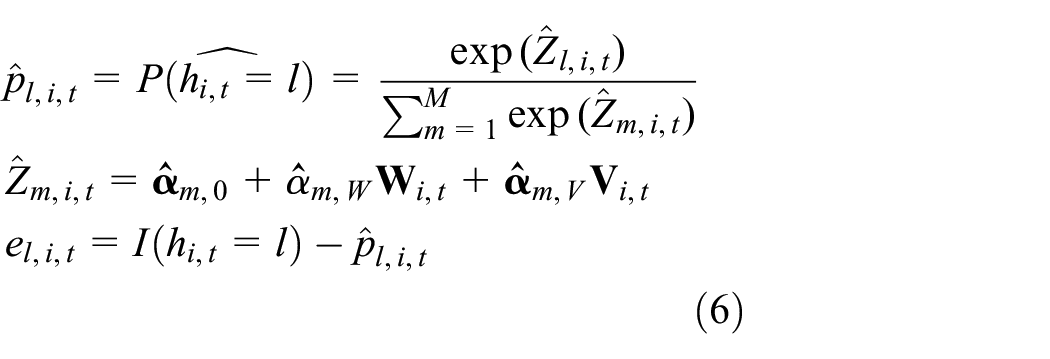
Then, we estimate the ordered logit model (1) by including the residuals on the right-hand side of the equation,
Intuitively, the predicted probability
To address the second issue, model (1b) is estimated by Baetschmann et al.’s (2015) blow-up and cluster (BUC) estimator. 7 The BUC estimator is based on conditional maximum likelihood (CML) estimator, which estimates the coefficients in the fixed-effects ordered logit model by dichotomising the ordered categorical variable at an arbitrary chosen cutoff point. The CML estimator is consistent but loses efficiency as it utilises only one cutoff point. The BUC estimator improves efficiency by maximising the sum of the conditional likelihoods created by dichotomising the ordered outcome at multiple cutoff points.
Findings
Housing tenure equation
The random-effect multinomial logit model of housing tenure choice in the first stage of 2SRI exhibits a close fit to the observed housing tenure data, with an overall predictive accuracy of 92.8%. At the bottom of Table 1, the IVs’ joint significance is not rejected, validating the variables’ relevance in predicting housing tenure status. Many of the IVs are also individually significant predictors of housing tenure. In Table 1, the receipt of parental transfers above AU$10,000 raises the odds of mortgaging, relative to the reference category of renting, by 88%. In contrast, receiving a small parental transfer (AU$1–10,000) contributes adversely towards purchasing a home. Having a father who is a professional, community and personal service worker, machinery operator or driver, or a labourer, instead of a manager, reduces the odds of becoming a mortgagor relative to a renter by 21% to 33%. Receiving a parental transfer does not influence the odds of outright owning relative to renting. However, the father’s occupation again matters for achieving outright ownership. As expected, the user cost of owning is negatively associated with the odds of achieving mortgaging and outright ownership relative to renting.
Random-effects multinomial logit model of tenure choice, instrumental variables only.
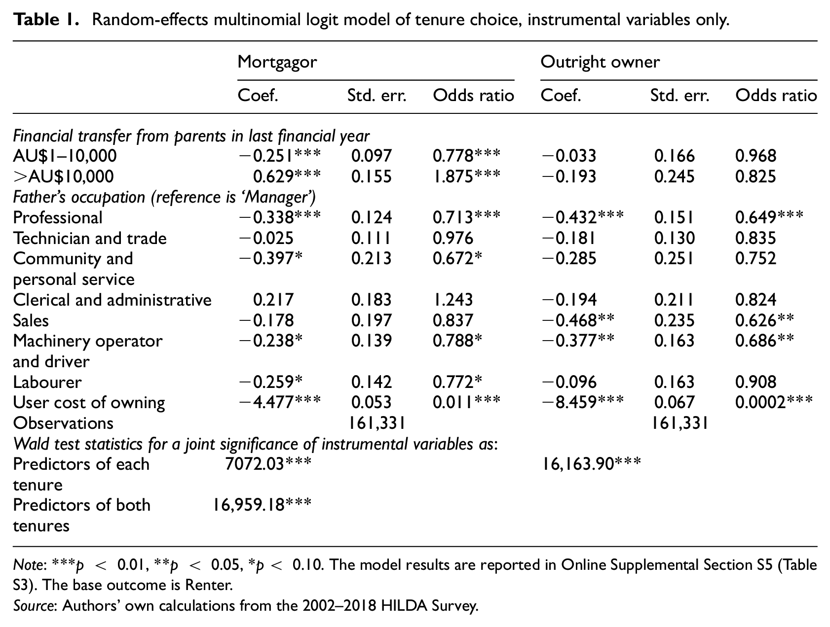
Note: ***p < 0.01, **p < 0.05, *p < 0.10. The model results are reported in Online Supplemental Section S5 (Table S3). The base outcome is Renter.
Source: Authors’ own calculations from the 2002–2018 HILDA Survey.
SWB equation – model specification and endogeneity test
Table 2 summarises the results from estimating the fixed-effects ordered logit model of four SWB domains across two specifications. Comparing the restricted and unrestricted specifications, we find that the value of the likelihood function is lower, while that of the Akaike Information Criterion is higher for the restricted model. The Wald test statistics in the table also indicate that the interaction terms between housing tenure and age, income, location and duration of current residence are jointly significant predictors of all the SWB domains, except for interaction terms involving mortgaging in the case of life satisfaction. 8 These results suggest that the effects of homeownership on four domains of SWB vary by age, income, location or duration of residence, albeit with weaker statistical support for the variational impacts of mortgaging on life satisfaction.
Summary of results from restricted and unrestricted SWB models.
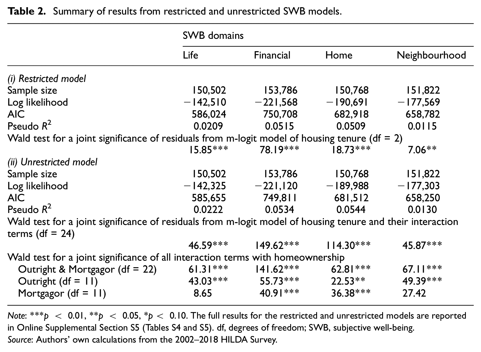
Note: ***p < 0.01, **p < 0.05, *p < 0.10. The full results for the restricted and unrestricted models are reported in Online Supplemental Section S5 (Tables S4 and S5). df, degrees of freedom; SWB, subjective well-being.
Source: Authors’ own calculations from the 2002–2018 HILDA Survey.
Table 2 also shows that the residuals from the housing tenure multinomial logit model and their interaction terms with age, income, location and duration of residence are jointly significant at a 1% level for all four SWB domains. These residuals carry information about housing tenure unrelated to the IVs or the covariates on the right-hand side of the housing tenure or SWB equations. Their significance proves the existence of endogeneity due to factors affecting both housing tenure and SWB that are not controlled for by the covariates in the SWB equations. Thus, the SWB equations estimated by the standard maximum likelihood method without including these residuals will yield biased and inconsistent estimates.
H1: SWB is higher for owners than renters. However, among owners, SWB is higher for outright owners than mortgagors
Table 3 summarises the results from statistically testing the four hypotheses. Firstly, in panel (H1-i) of Table 3, the coefficients of outright ownership and mortgaging in the restricted models of SWB are positive and significant for all SWB domains, albeit only at the 10% level for the effect of mortgaging on life satisfaction. These results support H1: homeownership increases all SWB across all four domains. The estimated coefficients are particularly large for home satisfaction, translating into odds ratios of 3.064 and 2.811 for outright owning and mortgaging, respectively. 9 That is, the odds of reporting higher home satisfaction scores relative to lower scores are around three times higher for owners than renters. The coefficient is also prominent for outright ownership on financial satisfaction, signifying the importance of homeownership in wealth accumulation.
Test statistics for hypotheses regarding homeownership’s impacts on SWB (H1) and its variation across location, age and income (H2–H4).
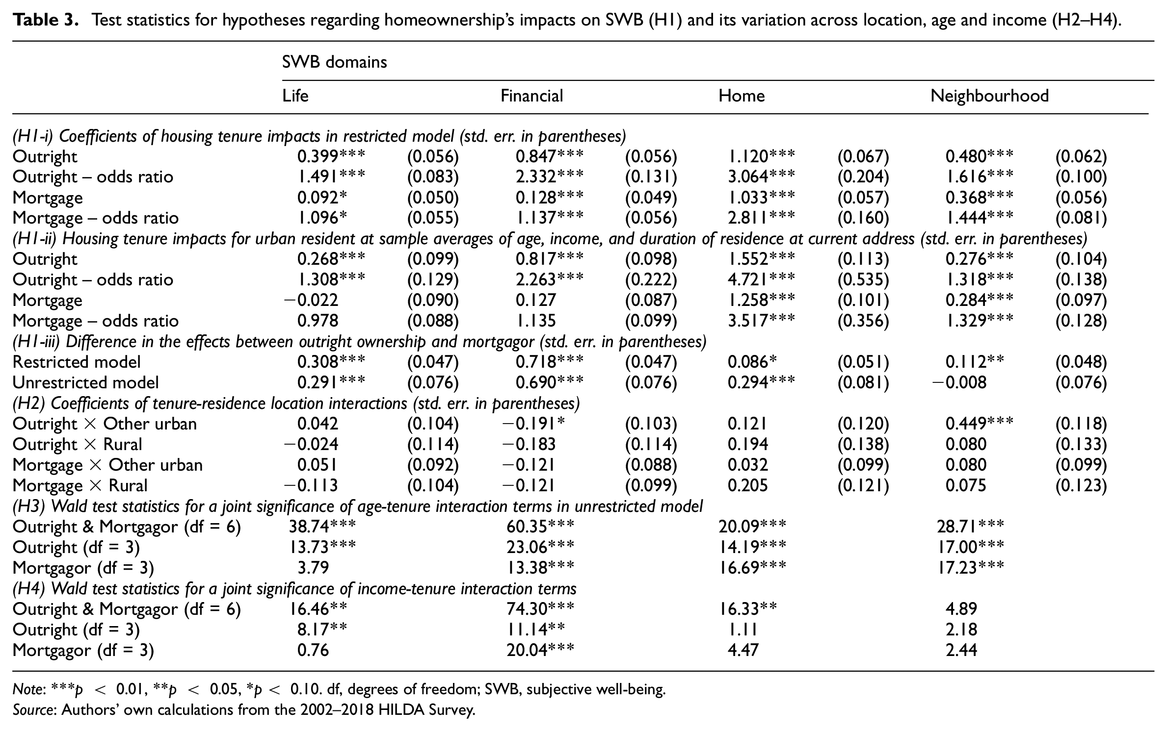
Note: ***p < 0.01, **p < 0.05, *p < 0.10. df, degrees of freedom; SWB, subjective well-being.
Source: Authors’ own calculations from the 2002–2018 HILDA Survey.
Panel (H1-ii) of Table 3 reports the unrestricted model’s predicted housing tenure impacts for an urban resident scoring sample means of age, income and duration of residence. The predicted patterns are similar to the restricted model, except that the effects of mortgaging on life and financial satisfaction are no longer significant.
For all SWB domains, the estimated coefficients are greater for outright owning than mortgaging in the restricted model. In panel (H1-iii), the differential effects evaluated at the sample means based on the unrestricted model are similar to the restricted model except that the differential effect is negative and insignificant for neighbourhood satisfaction. These results support the second part of H1; the difference in SWB between outright owning and renting is greater than mortgaging and renting, except for neighbourhood satisfaction.
H2: The positive SWB gap between owners and renters is smaller outside major urban locations than within major urban locations
The differential effect of homeownership on SWB by the location of residence is captured by the coefficients of the location-tenure interaction terms
H3: The positive SWB gap between owners and renters widens as age increases
Variation in housing tenure impacts across age is tested by the joint significance of the age–tenure interaction terms for each tenure type (l = 1 and 2) and each SWB domain. The results summarised in panel (H3) of Table 3 suggest that the effect of outright owning and mortgaging varies by age across all SWB domains, except that the variational effects of mortgaging by age are insignificant in the case of life satisfaction.
Figure 1 illustrates how the odds of achieving a higher satisfaction score relative to a lower score differs between renting and mortgaging and between renting and outright owning. It shows how these odds ratios vary by age and income while holding other predictors at their sample means. 10 In the figure, the predicted odds ratios and their 95% confidence intervals are given respectively by solid lines and grey bands for outright owners and heavy and light dotted lines for mortgagors.
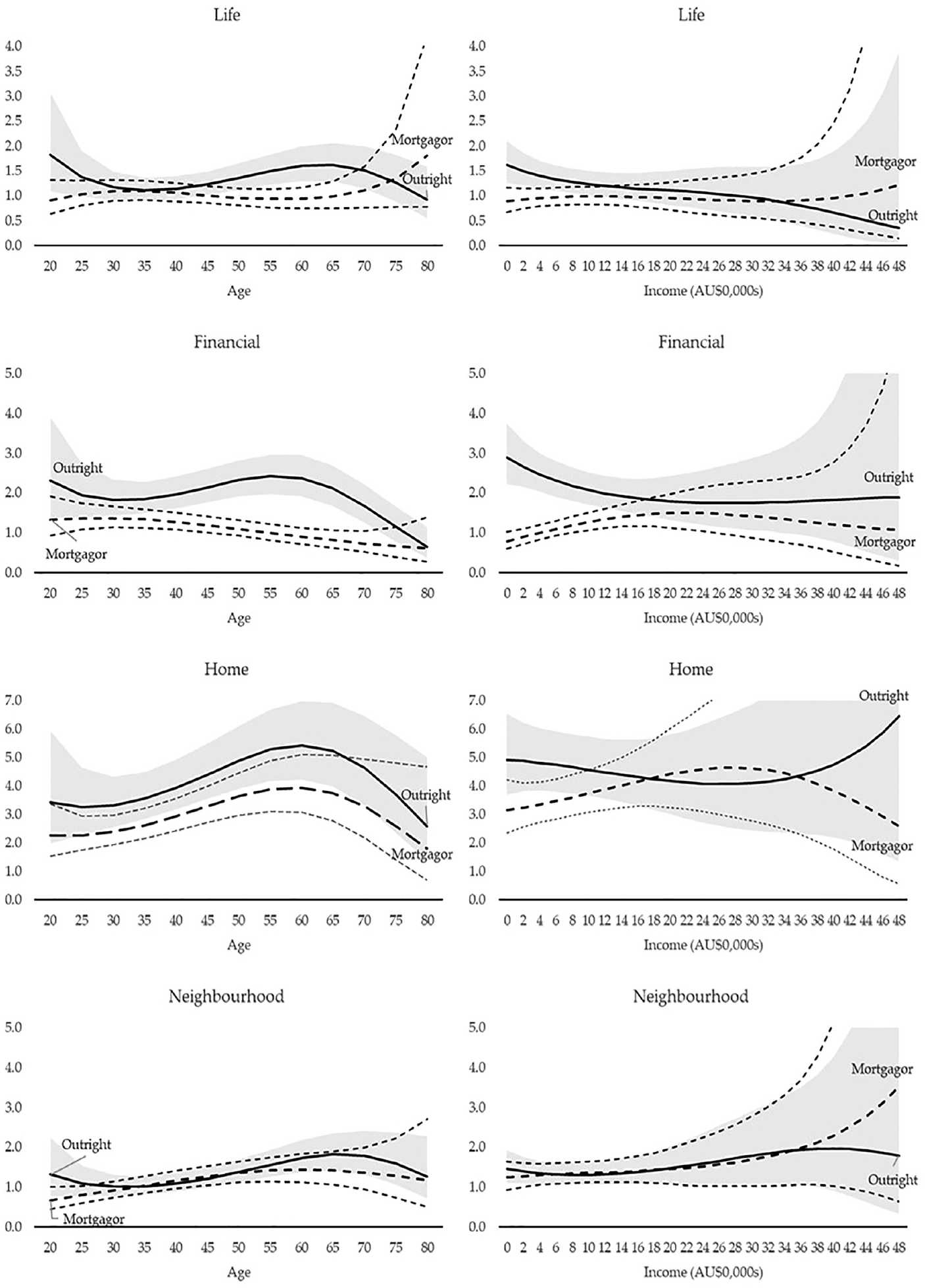
Predicted odds ratios of reporting higher SWB scores and its variation by age and income.
Before interpreting the results in Figure 1, we would note that tenure transitions are not distributed evenly across ages. Rather, as shown in Online Supplemental Section S4, as age increases, shifts from renting or mortgaging to outright owning become more likely, while shifts from mortgaging or outright owning back to renting become less likely. However, the sample still offers a healthy number of tenure transitions within each age group. Furthermore, in each of the eight panels in Figure 1, the confidence intervals usefully highlight the age and income ranges, whereby results do not fall within confidence bands.
First, on the left-hand side of Figure 1, the positive impact of homeownership is strongest in the domain of home satisfaction, where the odds of achieving a higher home satisfaction score relative to a lower score are substantially and significantly higher for outright owners and mortgagors than for renters (the odds ratio for homeowners to that for renters exceeds one) across the entire age range. For both owner tenures, the odds ratio rises from around age 30 to 60 before declining. This decline may reflect the growing physical burden of maintaining an owned home in old age, which depresses satisfaction with one’s home.
In the case of financial satisfaction, outright ownership is associated with an odds ratio above one across nearly the full age range. The positive financial satisfaction gap between outright owners and renters widens between ages 35 and 60. However, the negative impact of debt on financial satisfaction is illustrated by the positive but declining odds ratio associated with mortgaging, evident only in the 25–50 years range, where younger mortgagors feel more financially satisfied than their renting counterparts. Those carrying a mortgage debt past their prime working years have financial satisfaction levels not statistically different from renters, which possibly reflects the financial stress accompanying the need to make mortgage repayments while approaching retirement.
Positive and increasing life satisfaction is achieved only for outright owners (not mortgagors), increasing relative to renters for ages 35–65, after which the odds ratio declines but remains above one until age 75 years. Similar trends are observed for neighbourhood satisfaction associated with outright ownership. Most older people prefer to age in place, and this desire is more easily facilitated via homeownership than renting (Lee et al., 2019). However, elderly renters are primarily free from maintenance burdens that elderly homeowners carry despite growing physical limitations, potentially explaining outright owners’ diminishing life satisfaction in their 70s.
H4: The positive SWB gap between owners and renters narrows as income increases
The joint significance of income–tenure interaction terms tests the differential effects of homeownership by income level. The results reported in panel (H4) of Table 3 show a stark contrast to H3; variation across income is significant only for the effects of outright ownership on life and financial satisfaction and for mortgaging on financial satisfaction.
Figure 1 confirms these results, showing that the effects of outright ownership on life and financial satisfaction diminish monotonically with income. For financial satisfaction, the odds ratio of outright owning is significantly above one at a low-income level. It declines with income and becomes insignificantly different from one for income above AU$320,000. For mortgaging, the effect on financial satisfaction increases with income for an income range below AU$200,000, after which it declines and becomes insignificant for income above AU$240,000.
The financial satisfaction decline seems consistent with the observation that wealthier individuals have more diverse asset portfolios. According to the 2018 HILDA Survey, housing and superannuation assets made up, respectively, 66% and 10% of the total assets held by households in the AU$20,000–29,999 gross income range, while the corresponding numbers for the top end of the income distribution (with income above AU$200,000) are 39% and 20%, respectively. Thus, homeownership’s contribution to financial satisfaction is lower among those that are wealthier.
Conclusion
This article has investigated how the impact of homeownership on SWB varies by homeownership status, location, age and income in Australia. We find that homeownership, particularly outright ownership, has a positive effect on SWB – as measured by life, financial, home and neighbourhood satisfaction – relative to renting. However, as summarised below, these effects are not homogeneous. We review our findings against each hypothesis in turn.
Our findings offer support for Hypothesis 1. We find generally positive effects of homeownership on SWB, which are particularly strong in the case of home and financial satisfaction. Across all domains, the effects are generally stronger for outright ownership than for mortgaging. Hypotheses 2, 3 and 4 are only partially supported by our findings. Concerning Hypothesis 2, we find that outright owners in major urban locations enjoy higher financial satisfaction but poorer neighbourhood satisfaction than their counterparts living outside major urban locations. Regarding Hypothesis 3, the positive SWB gap between owners and renters does widen as age increases, but only over a limited age range (around the 30s to 60s). The negative impact of debt on financial satisfaction is reflected beyond age 50, where older mortgagors carrying debt past their prime working years have financial satisfaction levels not statistically different from renters. Turning to Hypothesis 4, as income increases, we find that the effects of outright ownership on life and financial satisfaction diminishes, as does the effect of mortgaging on financial satisfaction.
We highlight three relevant policy themes and link them to our key hypotheses in parentheses. First, the positive SWB impacts of homeownership are not homogeneous, so policies that seek to promote homeownership ought to be cognizant of its interactions with other factors that might depress the positive SWB impacts of ownership, such as lower house price appreciation rates outside major urban locations (Hypothesis 2), higher densities in major urban locations (Hypothesis 2) and the lack of tailored age-specific housing and care to support ageing in place for as long as possible (Hypothesis 3).
Second, the positive SWB impacts of homeownership are evident among outright ownership but much less so for mortgagors (Hypothesis 1) and, in fact, the positive financial satisfaction effects of mortgaging relative to renting disappear after age 50 (Hypothesis 3). Traditionally, this is of minor concern as mortgage debts are typically paid off by retirement. However, progressively more studies have highlighted rising mortgage indebtedness among Australian homeowners extending to those approaching and in retirement. The findings threaten the sustainability of homeownership as a key pillar of the retirement income system because the financial satisfaction premium attached to low-income homeownership is only evident in the case of outright ownership (Hypothesis 4). Thus, there is a need to further discourage the extension of debt holdings into later life when adverse life shocks, such as marital dissolution and ill-health, may derail mortgage repayment capacities.
A third and follow-on implication is the need to manage the risks of low-income homeowners whose asset portfolios, and hence their financial satisfaction, are heavily influenced by the owner-occupied home (Hypothesis 4). During a financial crisis, homeowners are often forced to sell with little time for proper planning or maximising of capital gain. It may leave some with little to no equity to rebound to homeownership, thus consigning them to the stresses of renting and dependence on rental housing assistance in old age.
Finally, we note that an obvious limitation of our study is that satisfaction indicators do not fully capture SWB, which is a multi-dimensional concept. A bank of studies exists examining the links between housing tenure and other aspects of SWB, such as mental health, including Baker et al. (2013), Mason et al. (2013) and Li et al. (2022). Thus, an important future research direction is to replicate the present study to determine whether the results hold for other SWB measures. There also remains significant scope to address potential age or cohort effects that may bias some results. Specifically, certain age groups may be over- or under-represented in the sample, and different generational cohorts would be making tenure decisions within different socio-economic backdrops, which may not have been fully accounted for in our models despite the inclusion of calendar years as predictors.
Supplemental Material
sj-docx-1-usj-10.1177_00420980231190479 – Supplemental material for Homeownership and subjective well-being: Are the links heterogeneous across location, age and income?
Supplemental material, sj-docx-1-usj-10.1177_00420980231190479 for Homeownership and subjective well-being: Are the links heterogeneous across location, age and income? by Rachel Ong ViforJ, Hiroaki Suenaga and Ryan Brierty in Urban Studies
Footnotes
Declaration of conflicting interests
The author(s) declared no potential conflicts of interest with respect to the research, authorship, and/or publication of this article.
Funding
The author(s) disclosed receipt of the following financial support for the research, authorship, and/or publication of this article: Rachel Ong ViforJ is the recipient of an Australian Research Council (ARC) Future Fellowship (project FT200100422) funded by the Australian Government. While conducting this research, Ryan Brierty has been supported by a 2021 Master of Research Stipend Scholarship and 2022 Curtin Higher Degree by Research Scholarship funded by Curtin University. This article uses unit record data from the Household, Income and Labour Dynamics in Australia (HILDA) Survey. The HILDA Project was initiated and is funded by the Australian Government Department of Social Services (DSS) and is managed by the Melbourne Institute of Applied Economic and Social Research (Melbourne Institute). The findings and views reported in this article, however, are those of the authors and should not be attributed to the Australian Government, ARC, DSS or the Melbourne Institute.
Supplemental material
Supplemental material for this article is available online.
Notes
References
Supplementary Material
Please find the following supplemental material available below.
For Open Access articles published under a Creative Commons License, all supplemental material carries the same license as the article it is associated with.
For non-Open Access articles published, all supplemental material carries a non-exclusive license, and permission requests for re-use of supplemental material or any part of supplemental material shall be sent directly to the copyright owner as specified in the copyright notice associated with the article.