Sage Journals: Discover world-class research

Abstract

Chinese

Recent years have seen growing concern about the ‘hollowing out’ of the middle class, due to processes of polarisation. In this paper, we examine different conceptualisations of polarisation, and introduce the concept of expenditure-adjusted polarisation that considers not only income, but also various key categories of expenditure at a household level: housing, groceries and meals, transport and energy. Analysing longitudinal data from the Household, Income and Labour Dynamics in Australia Survey, we show that the Australian society is significantly more polarised, with fewer middle-income households, when the relative size of income groups in a given year is based on expenditure-adjusted income rather than pre-expenditure income. Such polarisation is particularly prominent when housing expenditure is considered and has distinctive spatial patterns. In contrast, our analysis finds no evidence of a temporal pattern of polarisation in Australia between 2005 and 2019, with no substantial change in the size of income groups over time, regardless of which income measures are used. We argue that a more nuanced conceptualisation of polarisation, and its relation to processes of ‘hollowing out’ and rising inequality, is needed to inform urban scholarship and policy.

Keywords

after-housing income expenditure-adjusted polarisation HILDA housing tenure middle class

Introduction

The term polarisation is frequently used in media, political and scholarly discourses, its meaning varying from the divergence of political attitudes to ideological extremes, to changes in the socio-economic structure of society (Babones, 2008; Banerjee and Duflo, 2003). A common use of the term polarisation in economics is to denote growth in the proportion of both high- and low-income households, with a smaller proportion in the middle of the income distribution (Dinca-Panaitescu and Walks, 2015). The middle class drives consumption and entrepreneurship in the market, direct investment in public infrastructure and services such as education and health, and tax contributions which support various functions of the state (OECD, 2019). Therefore, the ‘squeezing’ or ‘hollowing out’ of the middle class has been described as a threat to the cohesion and prosperity of societies and cities.

The term social class encompasses material aspects (income and wealth) as well as non-material aspects (including relational and cultural considerations). In contrast to continuous-scale measures of individuals’ socio-economic standing, class analysis considers individuals and households in clusters (classes), and understands the structure of these clusters (such as their size, cohesion and relationship with other clusters) to be meaningful to individual identities and to social relations (Keister and Southgate, 2022). Polarisation is one lens through which the class structure can be explored.

The drivers of polarisation are subject to debate. The ‘global city’ thesis associated polarisation with globalisation (Sassen, 1991); however, recent evidence points to more complex and context-specific drivers (Hamnett, 2021). Either way, although costs of living outpacing wage growth has been acknowledged as one driver of polarisation (OECD, 2019), most analyses tend to focus on labour market drivers and changes to the occupational structure. Studies in North America and Europe attribute a hollowed out middle class to ongoing changes in the labour market and income that have been occurring since the 1970s (Autor et al., 2006; Goos et al., 2009). Coelli and Borland (2016) show that similar patterns of ‘job polarisation’, and associated changes in earnings, also occurred in Australia but predominantly during the 1980s and 1990s. Similarly, Wilkins and Wooden (2014) contend that there is little evidence of job polarisation in Australia between 2003 and 2013.

In this paper, we introduce the concept of expenditure-adjusted polarisation that recognises the uneven distribution of both income and expenditure, and their combined impact on processes of polarisation. Unlike previous literature that has emphasised the downward pressure of living costs on the middle class (OECD, 2019), our empirical study demonstrates that uneven expenditure – shaped to a large extent by urban geography and housing tenure inequalities – can propel households to either ‘slip down’ or ‘move up’ from the middle. In both cases, this can facilitate polarisation and a hollowing out of the middle class. We analyse longitudinal data covering the period of 2005–2019 from the Household, Income and Labour Dynamics in Australia (HILDA) Survey to examine variation in the size of Australia’s ‘lower’, ‘middle’ and ‘higher’ income groups, when accounting for income alone, and when deducting essential household expenditures on housing, groceries and meals, transport and energy. Our analysis shows that between 2005 and 2019, levels of income polarisation in Australia were more significant when adjusted to expenditure and showed distinctive spatial patterns when measured in pre-expenditure income, in measures adjusted to housing expenditure, and in measures adjusted to all essential expenditure. Acknowledging that income is only one aspect of social class position, we consider the implications of expenditure-adjusted income polarisation to the understanding of social class structures more broadly.

Polarisation: Pyramids, eggs and hourglasses

In the social sciences, the term ‘polarisation’ has been used to describe a concentration of people, resources or ideas across two opposite ‘poles’ or ends of a spectrum. Polarisation has also been described as a structure characterised by high levels of similarity within each cluster, and high levels of dissimilarity between clusters (Esteban and Ray, 1994). The concept has been applied in different, and at times inconsistent, ways. In this section we highlight four axes of difference in the way polarisation has been defined and measured. We then introduce a fifth axis in the concept of expenditure-adjusted polarisation, which we argue can help address a significant oversight in polarisation studies.

First, literature on political and ideological polarisation – and the related concept of affective polarisation – reflects a growing political divide within society, increased partisanship, attachment to political ingroups and hostility towards political others (Torcal and Comellas, 2022). In national politics, this often involves strengthening of political ideologies that are different from those of a so-called ‘median’ voter (Carrillo and Castanheira, 2008). Political and affective polarisation are not necessarily forms of inequality. However, some studies point to the interrelationship, whereby growing economic inequality reinforces cultural and political divides between the elite and those experiencing poverty and disadvantage (Gu and Wang, 2022). In social class terms, polarisation can be understood as increased cultural difference, and potentially also hostility, between different social classes as suggested by Holmqvist and Wiesel (2022).

Second, within analyses focused on material socio-economic polarisation, one significant distinction is between measures of polarisation focused on the distribution of people and occupations, and those focused on the distribution of income and wealth. Most studies on polarisation focus on the distribution of people across the socio-economic spectrum. Hamnett (2021), for example, describes historical changes to the social class structure of cities. Whereas pre-industrial and industrial cities’ class structure resembled a pyramid with a very small ruling class, a small middle class and a large working-class base, the post-industrial society has transformed into an egg-shaped structure due to significant expansion of the middle class and shrinking of the working-class base. However, some scholars – most notably Sassen (1991)– have argued that since the 1970s, a counter process has occurred whereby the squeezing of the middle class in global cities has transformed the egg into an hourglass. This has been described as a process of polarisation, driven by an increase in the share of high-skill and low-skill jobs and a decrease in middle-skill jobs, especially in global cities. These changes in occupational structure and earnings relate to technological change replacing routine cognitive and manual tasks previously undertaken by middle-skill workers, and also raising the productivity of high-skill workers who perform non-routine and interactive work involving information and communications technology (Autor et al., 2003).

Other measures of polarisation are concerned with the distribution of income or wealth across the socio-economic spectrum, with a particular focus on the most affluent groups (Bárcena-Martin et al., 2018; Roope et al., 2018). Polarisation, conceptualised and measured this way, is related and complementary to inequality, but also distinct from it (Chakravarty and D’Ambrosio, 2010). Measures of polarisation (such as the Wolfson Bipolarisation Index) examine the concentration of income on several focal or polar modes, whereas measures of inequality (such as the Gini coefficient) consider the overall dispersion of income distribution. However, empirically, there is often a high degree of correlation between the two (Ravallion and Chen, 1997; Rodríguez, 2006).

Third, whether income or wealth are used to measure affluence is another point of difference in the literature. While the wealth gap is typically greater than the income gap (Piketty, 2014), more studies have focused on income polarisation, partly because income data is often more readily available, and partly because of a strong focus on labour market dynamics, as discussed above. In Australia, wealth inequality, which includes housing and private financial assets including superannuation, is relatively low compared to other OECD countries (Dollman et al., 2015; Sila and Dugain, 2019). Importantly, both income and wealth are imperfect indicators of social class position, and do not capture other important dimensions of class position such as social and cultural capital, or subjective social class identification.

Fourth, most analyses focus on the temporal dimensions of polarisation, examining changes over time in the concentration of wealth or income. Others, however, are more attentive to the spatial expressions and drivers of polarisation, at global, national or urban scales. Urban geography has focused on how fundamental changes in occupational structure and income distribution have reshaped cities. Analyses have examined whether and how a more polarised socio-economic structure is reflected in the spatial organisation and dynamics within metropolitan areas. The term spatial polarisation is often used as synonymous with segregation, denoting high internal similarity and external dissimilarity between spatial clusters, at different scales (Johnston et al., 2016). Similarity and dissimilarity are typically measured in terms of the concentration of high income, or low income people in particular areas. In Australia, for example, much of this work has focused on processes of gentrification (growing concentration of higher-income workers in previously lower-income inner suburbs), and the suburbanisation of disadvantage (growing concentration of lower-income workers in middle and outer suburbs) (Gleeson and Randolph, 2002; Weller and van Hulten, 2012). In this paper, however, we expand the concept of spatial polarisation to also consider consistency in the size of the middle-income groups across different urban areas; our findings illustrate that a relatively even (or non-polarised) spatial distribution of middle-income households across the city can exist alongside a relatively uneven (or polarised) distribution of low- and high-income households.

Introducing expenditure-adjusted income polarisation

Expenditure-adjusted polarisation recognises that not only income and wealth, but also the costs of living are unevenly distributed across the population; and that this derives not only from differences in the living standards of the rich, middle and poor, but also from spatial and tenurial differences in the costs of essentials such as housing, food, energy and transport. This fifth axis relates to the notion of a ‘poverty penalty’ (Mendoza, 2011), which suggests poorer households spend more on essentials for various reasons, including living further from urban centres, increasing transport costs (Dodson and Sipe, 2008), or living in older, less energy-efficient homes, increasing energy costs (Buzar, 2007). In the United States, ‘food deserts’, characterised by poor access to healthy, affordable food, are another example of geographical poverty traps; however, their existence in other countries, including Australia, remains contested (Beaulac et al., 2009; Smoyer-Tomic et al., 2006). Having less time and ability to test the market, accessing imperfect information about the market, and being completely excluded from certain markets also contribute to the poverty penalty (Mendoza, 2011).

Importantly, even when low-income households pay less than higher-income households in absolute figures, this often equates to a larger proportion of income. In Australia, for example, households in the lowest-income quintile spent an average of 6.4% of disposable income on electricity and gas in 2018, compared to 1.5% by those in the top quintile (ACOSS and Brotherhood of St Laurence, 2018), despite having lower energy expenditure in dollar terms. Similarly, food expenditure increases with household income, as wealthier households buy higher-quality food items and more convenience foods; however, poorer households spend a greater share of their income on food than wealthier households (Kaufman et al., 1997).

While the ‘poverty trap’ is primarily concerned with low-income households – and the risk of sliding below the poverty line – there is also literature examining the impact of rising costs of living on the middle class – and the risk of sliding below a middle-class living standard. A key focus of this research has been the rising costs of health, education and housing above inflation and wage growth, disproportionately impacting on middle-class households in large urban areas (OECD, 2019: 24).

Housing is a primary driver of expenditure-adjusted polarisation, as both the largest household expenditure category, and one in which significant disparities in costs exist across geographical areas and across tenures. Hamnett (1984) and Bentham (1986) in a UK context in the 1980s, and later Winter and Stone (1998) in Australia, identified such processes as socio-tenurial polarisation. In Australia, more recent work has shown that there is a high proportion of renters and mortgaged home-owners in the lower end of the income distribution, compared with a higher proportion of outright owners in the upper end. As a consequence, expenditure on housing as a proportion of income is significantly higher for lower-income households. In turn, the gap between the highest and lowest quintiles widens substantially when measured in ‘after-housing income’ (with housing costs deducted from disposable income) compared to ‘pre-expenditure income’ (Wiesel et al., 2023). Previous research has shown the extent to which housing expenditure pulls low-income households, especially those in the private rental sector, below the poverty line (Hulse and Burke, 2000; Saunders et al., 2022).

One critical challenge in analysing expenditure-adjusted income polarisation is that high expenditure has different meanings and implications across the income spectrum. For low-income households, high expenditure on housing or groceries and meals may reflect difficulty in meeting necessary household needs and can be interpreted as evidence of disadvantage; in contrast, for wealthy households, high expenditure can suggest discretionary spending based on a desired standard of living. What counts as ‘essential’ expenditure, and what is discretionary, is also difficult to define and measure. Furthermore, high expenditure in one category can be offset by reduced expenditure in another. For example, paying more on housing in a central metropolitan location may lead to reduced expenditure on transport. This calls for analysis that examines different expenditure categories, and their interdependencies.

In the following sections we turn our attention to changing patterns of expenditure-adjusted income – in different cities, different urban locations and at different time points – and examine whether and how these reveal patterns of polarisation. What evidence is there of expenditure-adjusted polarisation in Australia, and in its major cities in particular? Does it involve a hollowing out of middle-income groups, and what happens to those households (e.g. do they ‘slip down’ or ‘move up’ from the middle)? How does expenditure-adjusted polarisation change, or how is it influenced by, the geography of cities?

Methods

Data source and study population

Data used in this analysis are from the Household, Income and Labour Dynamics in Australia (HILDA) Survey. The HILDA Survey is a broad economic and social longitudinal study, which began with a large nationally-representative sample of Australian households occupying private dwellings in 2001 (Summerfield et al., 2020). The first wave includes responses from 13,969 individuals from 7,682 households, who form the basis of the panel followed in subsequent waves. Evolution of this sample over subsequent waves reflects children born or adopted; new immigrants joining enrolled households; departure of ‘Temporary Sample Members’ who joined households after the original sampling; attrition due to survey non-response, households moving out of scope or deaths; and the addition of 2,153 new households through a sample top-up to increase representativeness in 2011. By 2019, the responding sample comprised 23,237 individuals from 9,664 households.

Aside from Figure 1, which presents trends in mean income and expenditure between 2002 and 2019, our analysis was performed on selected waves of the HILDA Survey data from 2005, 2011, 2015 and 2019, based on the availability of expenditure data across waves. Changes to the questionnaires over time meant that data on some household expenditure categories were not available in all years. Grocery and meal expenditure was absent from wave 2 and waves 6–10, while transport and energy expenditure were not included prior to wave 5. We retained one observation of a household each year, excluding observations of other household members. This selection ensured all households are weighted equally in our analysis on household-level variables. In addition, we excluded the household-year observations of those who had their residential location in a Statistical Area Level 3 (SA3) spatial unit for which fewer than 10 unique households were observed in the given wave of the HILDA Survey. We also excluded from the sample of analysis the households in the highest and lowest 1% of both equivalised and non-equivalised household income, to minimise distortion of income group cut-offs and group-level analyses associated with outliers.

Figure 1.

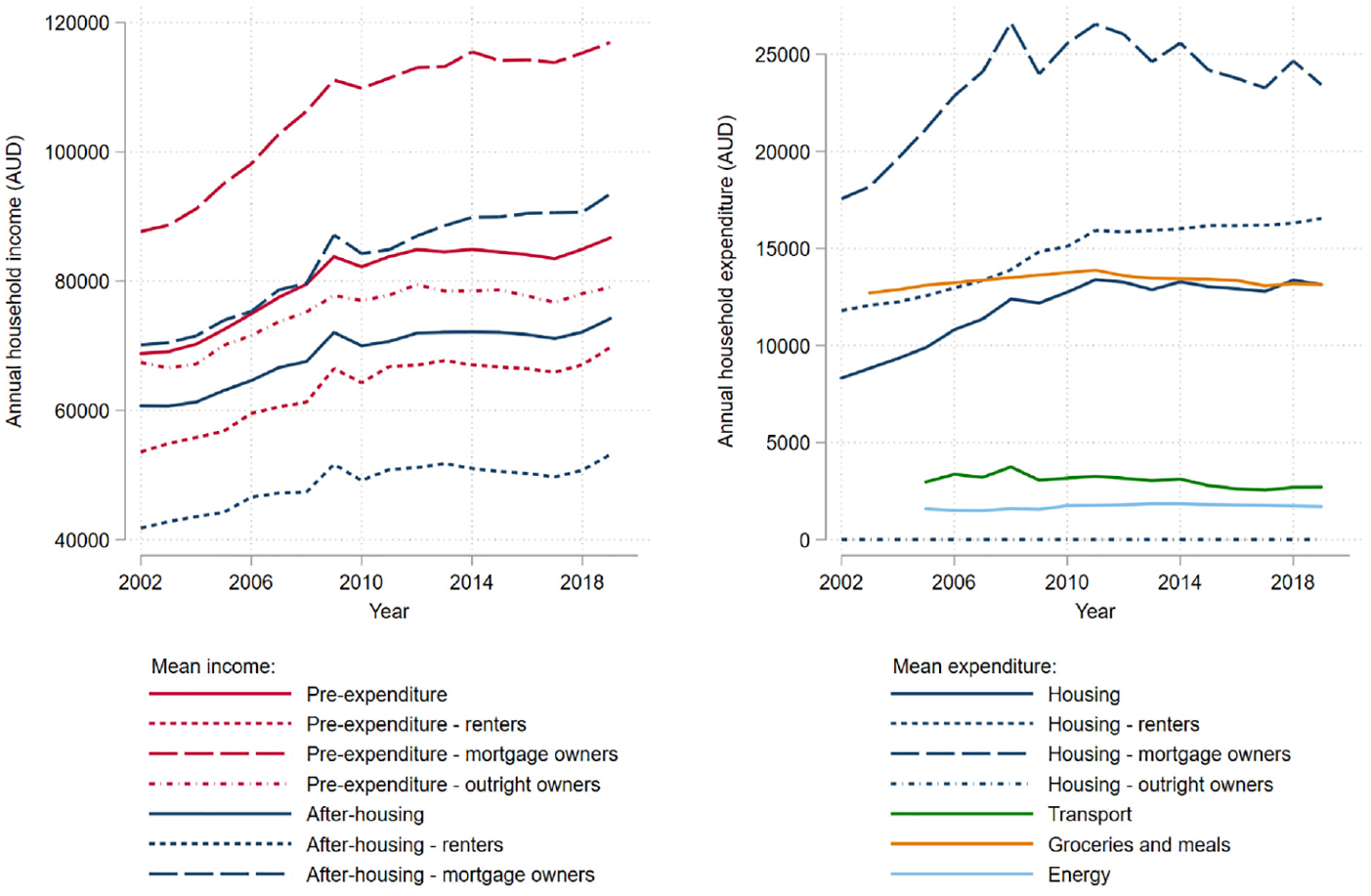
Average household income and expenditure over time.

Key variables

Table 1 presents variables considered in this study. All income variables and expenditure category variables are deflated by the consumer price index, and expressed in real terms in 2019 Australian dollars. Households are divided into three groups based on their housing tenure: renters, owners with a mortgage and outright owners. We distinguish home-owners based on whether or not they report mortgage repayments on their main home.

Table 1.

Variables considered in the analysis.

Description	Details
Pre-expenditure income	Annual household income
Real income	Adjusted for inflation
Equivalised real income	Adjusted for inflation and for number and age of household members (used in income group calculations)
Expenditure-adjusted income	Annual equivalised income less annual expenditure, both adjusted for inflation, for categories below:
a. Housing	Household rent or mortgage payments
b. Groceries and meals	All groceries and meals purchased outside the home
c. Transport	Motor vehicle fuel, public transport and taxis
d. Energy	Electricity bills, gas bills and other heating fuel
e. Essentials	Housing + Groceries and meals + Transport + Energy
Year	Year of data collection
Location	Household location, by ASGS Statistical Area Level 3 (SA3)
Housing tenure	Renter
	Owner with mortgage
	Outright owner
Income categories	Three groups, cut-offs relative to national median equivalised income
a. Lower-income	Less than 75% median household income
b. Middle-income	75–200% median household income
c. Upper-income	More than 200% median household income

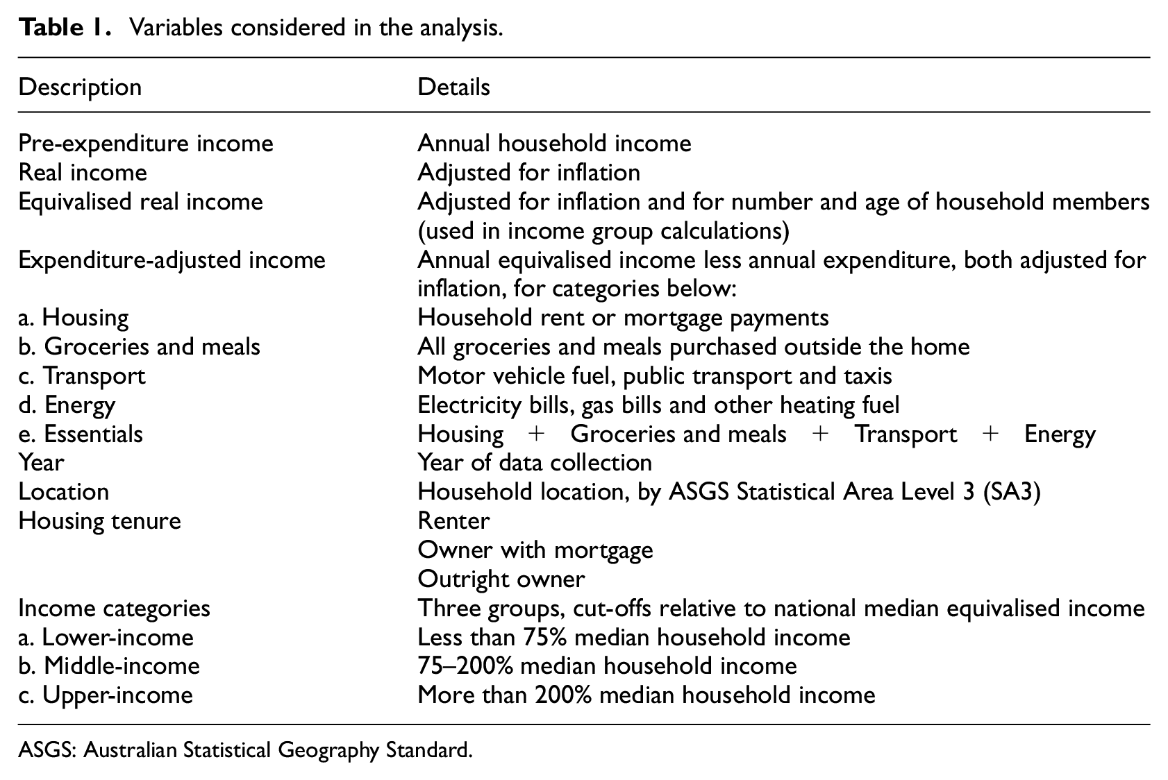
ASGS: Australian Statistical Geography Standard.

The spatial unit used is SA3, described as ‘functional areas of regional towns and cities with a population in excess of 20,000 or clusters of related suburbs around urban commercial and transport hubs within the major urban areas’ (ABS, 2021). Of 358 SA3 regions in Australia, our analysis includes households from 261 in 2005, as several SA3s, predominantly in rural areas, did not satisfy the minimum number of 10 household-year observations.

Social class encompasses economic and cultural dimensions; however, our analysis in this paper is limited to income (and expenditure) as one aspect and indicator of class position. We acknowledge that indicators used to define class structures vary widely, including across academic disciplines, but typically fall into three categories, based on (i) economic resources, including income and wealth; (ii) educational attainment or occupational status; and (iii) attitudes, behaviours or self-perception (Reeves et al., 2018). As outlined in Table 1, our analysis uses income groups, as a proxy for social class, which allows for temporal and spatial comparisons (OECD, 2019). The use of income as an indicator of class position is common practice, but we acknowledge the limitations of this approach, which excludes wealth as a component of economic resources and excludes other non-material aspects of social class. We return to the implications of these limitations in the paper’s conclusion.

Analysis

Descriptive analyses were performed to characterise the study sample, including summary statistics to reflect the distribution of the sample across states, household composition, housing tenure and mean household income and expenditure, by year.

To define income groups, we equivalised household income based on the number and age of household members. Following the OECD modified equivalence scale (Hagenaars et al., 1995), the formula used was 1 + 0.5 × (number of household members 14 yearsof age or above – 1) + 0.5 × number of household members less than 14 yearsof age. OECD (2019) thresholds were used to establish three income groups using equivalised household income: lower-income (less than 75% of national median income), middle-income (75 of age or above −200% of median) and higher-income (over 200% of median). Unlike measures which define income groups based on absolute income thresholds, or as static proportions of households within the income distribution (e.g. the middle 60% of the income distribution), the OECD (2019) thresholds allow analysis of changes in the relative size of lower, middle- and higher-income groups. Their consistency in the measurement of relative poverty also allows comparison between different societies, and between different points in time.

Income categories were also defined using alternative measures of household income: total disposable income (pre-expenditure) and with selected categories of expenditure deducted (expenditure-adjusted). Cut-offs were defined separately for each income measure and for each year. For example, income categories for after-housing income were established relative to the median national after-housing income in each of the four waves of included questionnaire data (i.e. 2005, 2011, 2015 and 2019). Income categories based on pre-expenditure income and after-housing income were also established for a sub-sample of households in Greater Melbourne and Greater Sydney. We examined how the size of income categories vary between income measures, over time, between locations and according to housing tenure. Results are reported based on percentage point (pp) differences.

We also assessed spatial and temporal patterns in the percentage of middle-income households at SA3-level in Greater Melbourne and Greater Sydney. Maps were generated to reflect the percentage of middle-income households by SA3 in 2019, as well as the percentage point change over this time period, using (i) pre-expenditure income, (ii) after-housing income and (iii) after-essentials income. This illustrates the complex patterns of spatial polarisation which are only apparent when expenditure is accounted for.

Results

The number of households included in the analyses ranged from 6,777 to 9,175 across the four waves of survey data, with an increase in 2011 corresponding to the recruitment of additional households in this year (Table 2). Mean household size was stable across the four waves, at 2.4–2.5 members (SD 1.4). The prevalence of home ownership decreased from 68.6% in 2005 to 63.3% in 2019.

Table 2.

Overview of the study sample, by year.

	Year of data collection
	2005	2011	2015	2019
Number of households (#)	6,777	9,088	9,203	9,175
Number of included SA3 regions (#)	261	277	281	283
Location of study sample (%)
New South Wales
Greater Sydney	16.8	17.3	16.5	15.4
Rest of state	14.2	13.5	13.3	13.5
Victoria
Greater Melbourne	17.2	16.9	17.4	17.7
Rest of state	7.1	7.1	7.6	7.8
Queensland
Greater Brisbane	8.8	9.4	9.9	10.4
Rest of state	11.4	11.6	11.7	11.4
South Australia
Greater Adelaide	6.5	6.7	6.8	6.6
Rest of state	2.9	2.7	2.6	2.5
Western Australia
Greater Perth	7.8	7.7	7.1	7.4
Rest of state	2.1	1.7	1.5	1.6
Tasmania	3.1	3.1	3.1	3.2
Northern Territory	0.4	0.5	0.6	0.6
Australian Capital Territory	1.8	1.9	2.0	2.0
Household characteristics
Number of members, mean (SD)	2.5 (1.4)	2.5 (1.4)	2.4 (1.4)	2.4 (1.4)
By housing tenure (%)
Renting	31.4	34.7	36.1	36.7
Own with mortgage	29.7	31.4	31.7	32.1
Own outright	38.9	33.9	32.2	31.2
Mean annual income ($)*
Overall income	72,490	83,791	84,510	86,695
Overall income, equivalised	44,121	50,799	51,605	53,275
Mean annual expenditure ($)*
Housing	9,894	13,389	13,027	13,132
Renting	12,557	15,933	16,171	16,550
Owners (overall)	9,175	12,769	12,005	11,880
Owners with mortgage	21,161	26,554	24,181	23,430
Groceries and meals	13,104	13,882	13,411	13,140
Transport	2,974	3,267	2,786	2,706
Energy	1,584	1,764	1,802	1,708

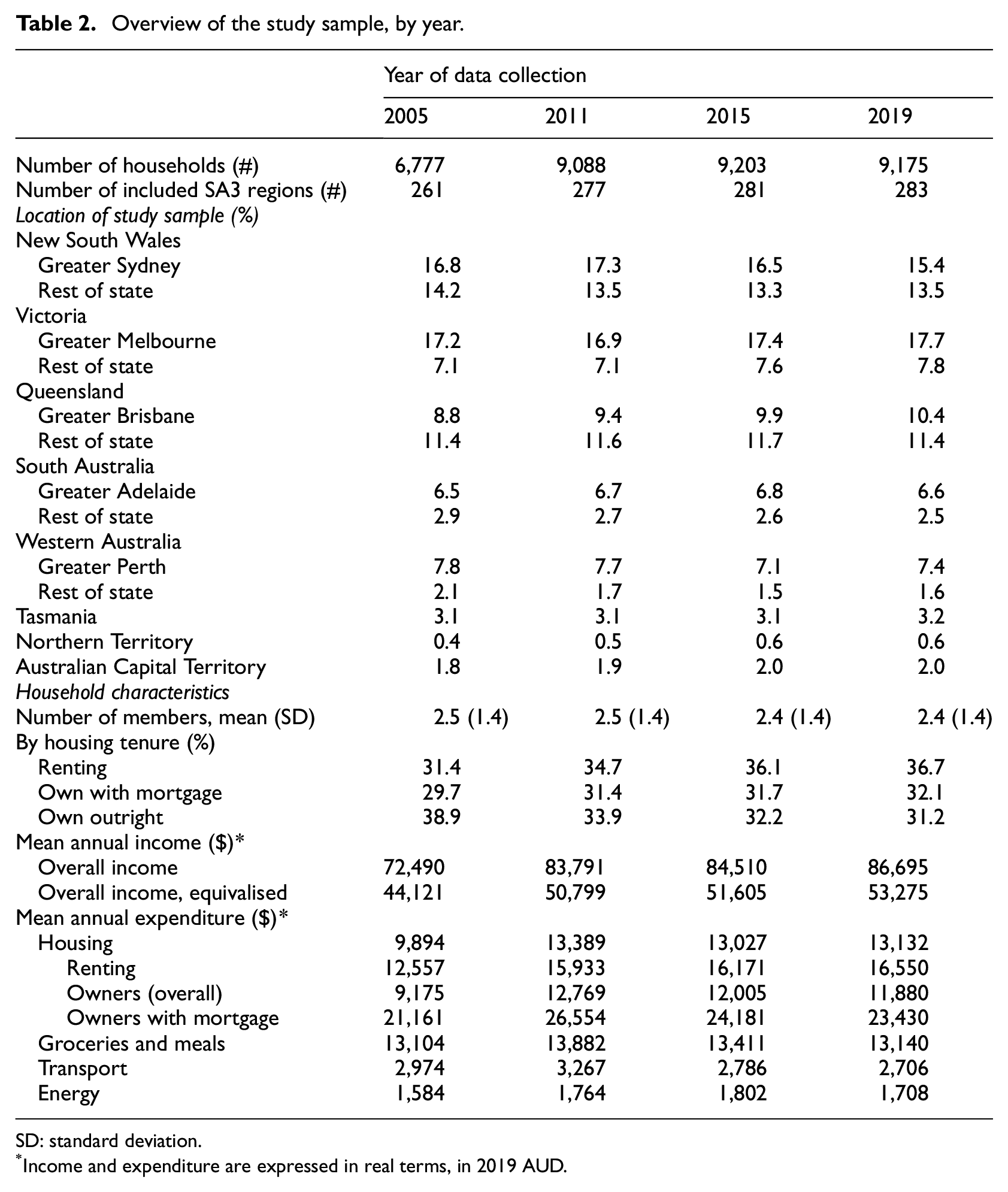
SD: standard deviation.

Income and expenditure are expressed in real terms, in 2019 AUD.

Pre-expenditure income

Mean annual household income amongst survey respondents increased from $72,490 in 2005 to $86,695 in 2019, in real terms, with the standard deviation rising from $46,979 to $54,414 across this period. Based on pre-expenditure income, the size of income categories remained relatively unchanged over the study period. The distribution resembled the egg structure, with a relatively large and steady middle-income group including 59.5% of study households in 2019, compared with 58.4% in 2005 (Table 3). However, a substantial difference in income profiles according to housing tenure was evident, with 40.8% of renting households classified as lower-income, 54.9% as middle-income and 4.2% as higher-income in 2019, compared with 11.3%, 75.5% and 13.2%, respectively, for mortgaged owners. As evident in Figure 1, growth in pre-expenditure real income has stagnated since 2009. This is consistent with the observation that real wages growth in Australia significantly slowed after 2008 (Kalb and Meekes, 2021).

Table 3.

Percentage of study sample in lower-, middle- and higher-income categories* based on equivalised real income, overall and after various categories of household expenditure, by year.

	Year of data collection
	2005	2011	2015	2019
Pre-expenditure income
Lower-income (<75% median)	32.8	32.0	32.2	31.8
Middle-income (75–200% median)	58.4	58.1	58.9	59.5
Higher-income (>200% median)	8.8	9.9	8.9	8.7
By housing tenure
Renting
Lower-income	41.2	41.6	42.1	40.8
Middle-income	53.2	52.6	52.7	54.9
Higher-income	5.6	5.8	5.2	4.3
Own with mortgage
Lower-income	13.5	12.9	12.8	11.3
Middle-income	74.6	72.7	74.6	75.5
Higher-income	11.9	14.4	12.6	13.2
Own outright
Lower-income	38.8	38.1	38.0	39.9
Middle-income	51.8	51.6	51.9	50.4
Higher-income	9.4	10.3	10.1	9.7
For selected locations
Greater Melbourne
Lower-income	28.6	25.5	26.0	25.2
Middle-income	60.3	63.4	63.2	63.5
Higher-income	11.1	11.1	10.8	11.3
Greater Sydney
Lower-income	26.7	30.4	30.3	28.3
Middle-income	59.4	56.7	58.7	59.8
Higher-income	14.0	12.9	11.0	11.9
After-housing income
Lower-income	33.6	34.8	33.4	33.8
Middle-income	49.0	47.1	49.0	49.4
Higher-income	17.4	18.1	17.6	16.8
By housing tenure
Renting
Lower-income	50.1	52.3	53.5	52.2
Middle-income	42.1	40.4	39.9	42.3
Higher-income	7.7	7.3	6.6	5.5
Own with mortgage
Lower-income	34.5	35.0	30.2	27.4
Middle-income	54.2	52.1	56.1	58.1
Higher-income	11.3	12.9	13.7	14.6
Own outright
Lower-income	22.5	20.4	18.0	22.5
Middle-income	54.9	54.4	57.7	54.4
Higher-income	22.6	25.3	24.3	23.1
For selected locations
Greater Melbourne
Lower-income	33.3	36.0	31.9	32.3
Middle-income	45.7	40.9	45.7	45.7
Higher-income	21.0	23.2	22.4	22.0
Greater Sydney
Lower-income	38.7	44.6	42.4	41.1
Middle-income	37.6	33.9	35.6	36.9
Higher-income	23.6	21.5	21.9	22.0
After-groceries and meals income
Lower-income	37.3	36.7	36.4	36.0
Middle-income	46.1	47.6	49.6	50.2
Higher-income	16.6	15.6	14.0	13.8
After-transport income
Lower-income	33.6	33.2	33.1	32.6
Middle-income	56.1	55.8	57.1	57.6
Higher-income	10.3	11.0	9.8	9.8
After-energy income
Lower-income	33.3	32.5	32.7	32.5
Middle-income	57.1	57.0	57.7	58.2
Higher-income	9.6	10.5	9.6	9.3
After-essentials income
Lower-income	40.8	41.3	39.9	39.4
Middle-income	29.7	28.6	32.5	33.7
Higher-income	29.5	30.1	27.6	26.9

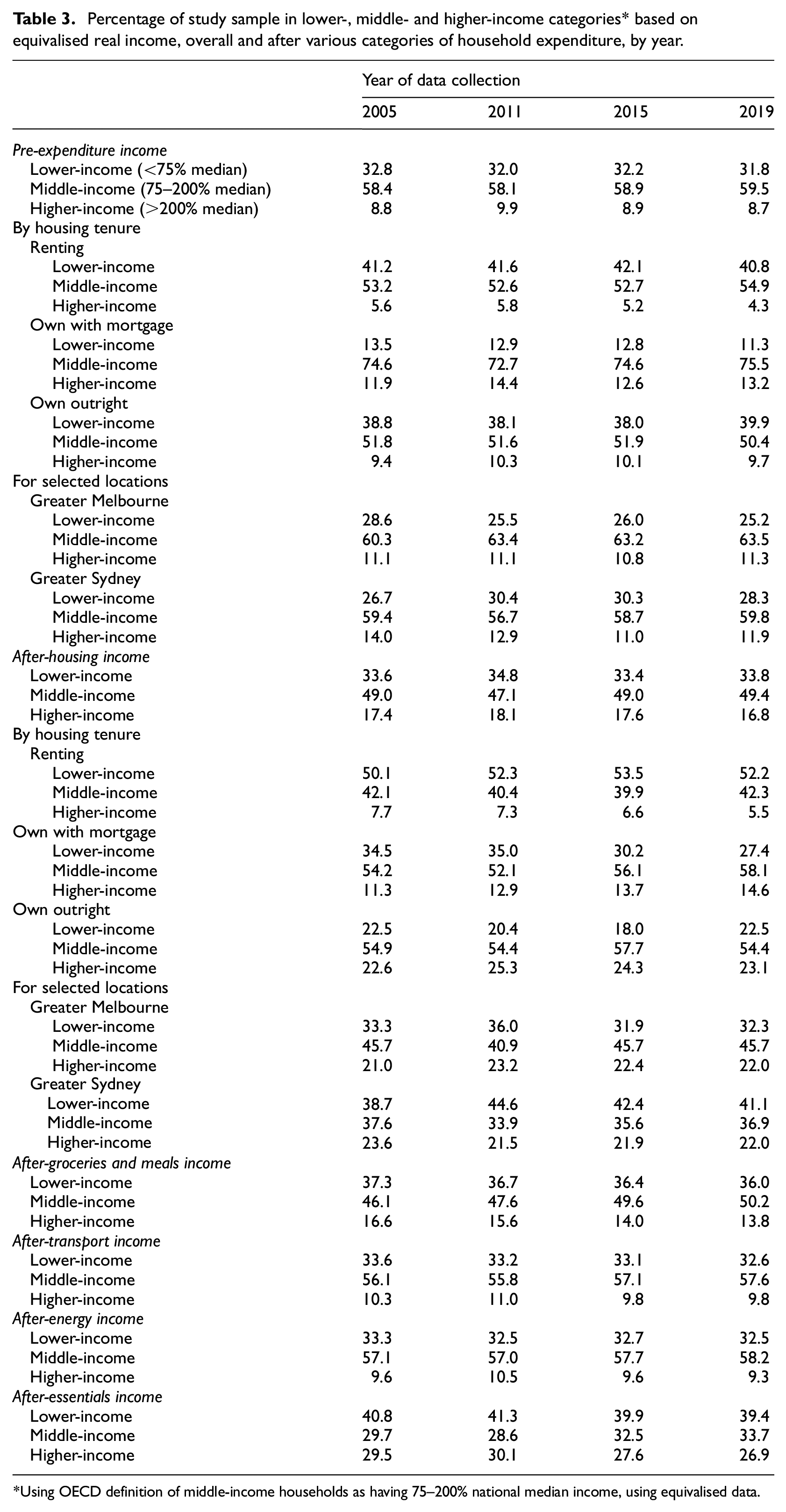
Using OECD definition of middle-income households as having 75–200% national median income, using equivalised data.

Expenditure-adjusted income

A more polarised social structure became evident when certain categories of expenditure were taken into account. Figure 1 and Table 2 show that, in real terms, average housing expenditure rose by around one-third (32.7%) between 2005 and 2019, compared to a smaller increase in energy expenditure (7.7%), a small reduction in transport expenditure (−9.0%) and relatively stable expenditure on groceries and meals outside the home (0.3%).

Table 4 presents a series of comparisons in the relative size of the middle-income group, testing the potential for polarisation to be identified when alternative measures were used. Housing and ‘groceries and meals’, the two main categories of household expenditure, were shown to be key drivers of expenditure-adjusted polarisation. When comparing pre-expenditure and expenditure-adjusted income at the same time point (2019), we observed a 10.1 percentage point (pp) reduction in the size of the middle-income category after accounting for housing expenditure, and a 9.3 pp reduction after accounting for groceries and meals. This compares with after-transport and after-energy income, where the middle-income category was only reduced by 1.9 pp and 1.3 pp, respectively. Housing expenditure was associated with ‘upwards’ polarisation pressure (i.e. a larger increase in higher-income households), due to relatively low expenditure on housing by outright homeowners. In contrast, groceries and meals expenditure led to middle-income households being reclassified more evenly into both the lower- and higher-income categories. When accounting for all essential expenditure, the middle-income category was reduced by 25.8 pp.

Table 4.

Percentage point (pp) difference in size of middle-income category, using alternative income measures, based on different waves of survey data, housing tenure and location.

(a) Difference (pp) with pre-expenditure income	2005	2011	2015	2019
After-housing income
Overall	−9.4	−11.0	−9.9	−10.1
Renting	−11.1	−12.2	−12.8	−12.6
Own with mortgage	−20.4	−20.6	−18.5	−17.4
Own outright	+3.1	+2.8	+5.8	+4.0
After-groceries and meals income	−12.3	−10.5	−9.3	−9.3
After-transport income	−2.3	−2.3	−1.8	−1.9
After-energy income	−1.3	−1.1	−1.2	−1.3
After-essentials income	−28.7	−29.5	−26.4	−25.8
(b) Difference (pp) 2005–2019
Pre-expenditure income				+1.1
After-housing income
Overall				+0.4
Renting				+0.2
Own with mortgage				+3.9
Own outright				−0.5
After-groceries and meals income				+4.1
After-transport income				+1.5
After-energy income				+1.1
After-essentials income				+4.0
(c) Difference (pp) with national sample
Pre-expenditure income
Greater Melbourne	+1.9	+5.3	+4.3	+4.0
Greater Sydney	+1.0	−1.4	−0.2	+0.3
After-housing income
Greater Melbourne	−3.3	−6.2	−3.3	−3.7
Greater Sydney	−11.4	−13.2	−13.4	−12.5

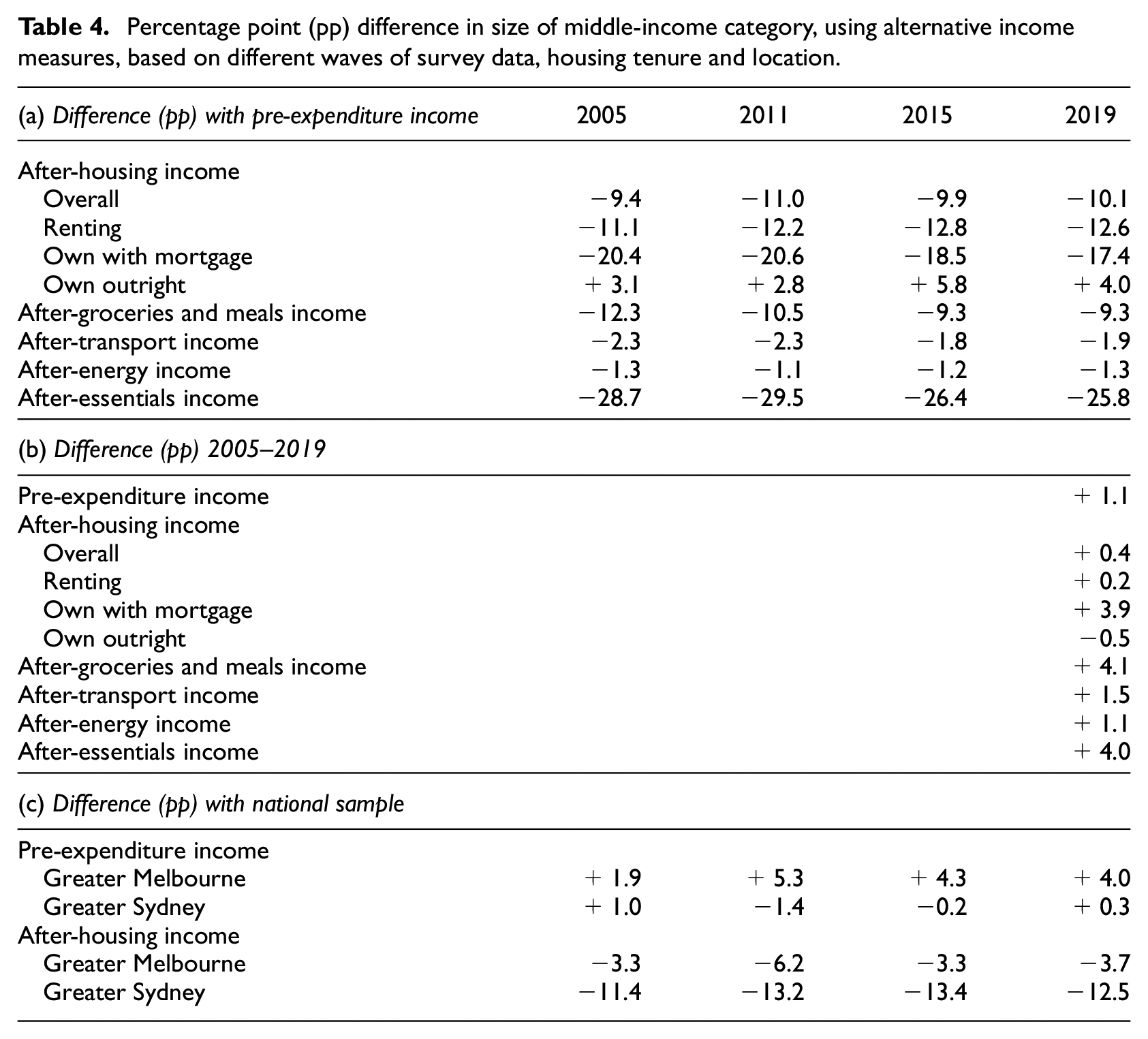
We found no evidence of significant polarisation over time in either pre-expenditure or expenditure-adjusted income. Between 2005 and 2019, we observe a small shrinkage of only 0.5 pp in the middle-income category for outright owners and a decrease of 0.7 pp among middle-income households in Greater Sydney (as discussed in the following subsection). Using income measures adjusted for groceries, transport and energy expenditure, the size of the middle-income group increased slightly over time (+4.1 pp, +1.5 pp and +1.1 pp, respectively, between 2005 and 2019). Similarly, when income was adjusted to all essential expenditure categories together, the middle-income group grew by 4.0 pp, while the higher and lower income groups became smaller by 2.6 pp and 1.4 pp respectively (Tables 3 and 4(b)).

Housing tenure played an important role in mediating expenditure-adjusted income polarisation. Examining the size of the middle-income group in pre-expenditure income, a significant disparity is apparent between mortgaged owners (of whom 72.7–75.5% are middle-income across the four years of included data; Table 3), and outright owners (50.4–51.9%) and renters (52.6–54.9%). Using after-housing income changes this pattern. In 2019, the proportion of middle-income households is 12.6 pp smaller for renters and 17.4 pp smaller for mortgaged owners than when measured using pre-expenditure income (Table 4(a)). By comparison, the size of the middle-income group is 4.0 pp larger for outright owners, when measured using after-housing rather than pre-expenditure income (Table 4(a)). Prominent differences were also seen in the direction of movement between income categories, with the loss from the middle almost entirely absorbed by the lower-income group for renters (+11.4 pp in 2019) and mortgaged owners (+16.1 pp) as shown in Table 3. In contrast, among outright owners, the gains in the middle-income group (+4.0 pp) are associated with a significant reduction in the proportion of lower-income households (−17.4 pp). There is also a notable increase in the proportion of higher-income outright owners (+13.4 pp). This reveals renting and mortgaged households to be ‘slipping down’ from the middle-income group, while owners without mortgage payments are ‘moving up’ both into and out of the middle-income group, when comparing pre-expenditure and after-housing income at a single time point. Over time, from 2005 to 2019, in pre-expenditure income, there were only small changes in the proportion of middle-income households across the tenure categories (Table 4(b)).

Spatial patterns of polarisation

Analysis of selected capital cities highlights geographic variation in the extent of income polarisation. Comparing Greater Sydney and Greater Melbourne in 2019, for example, Sydney was a more polarised city, with a smaller middle-income group compared to Melbourne (59.8% and 63.5%, respectively; Table 3) based on pre-expenditure income. When comparing the relative size of income categories in each city to the national sample, Melbourne had a slightly higher proportion of middle-income households based on pre-expenditure income (+4.0 pp) but a lower proportion based on after-housing income (−3.7 pp). This pattern was more prominent in Sydney, where the middle-income category was of a comparable size to the national sample using pre-expenditure income (+0.3 pp), but where a marked difference was observed in after-housing income (−12.5 pp; Table 4(c)).

In Melbourne, pre-expenditure middle-income households are relatively evenly spread across the metropolitan area (Figure 2). Figure 3 shows how the percentage of middle-income households within an SA3 area changes when based on expenditure-adjusted income rather than pre-expenditure income. Using after-housing income, there is a noticeable reduction in the proportion of middle-income households in the inner and middle suburbs. In after-essentials income, the proportion of middle-income households is further reduced across the whole metropolis, with particularly marked declines in the outer suburbs. These declines in the outer suburbs are driven by expenditure on transport, as expected, but also energy bills and groceries and meals, and/or relatively low income in these suburbs.

Figure 2.

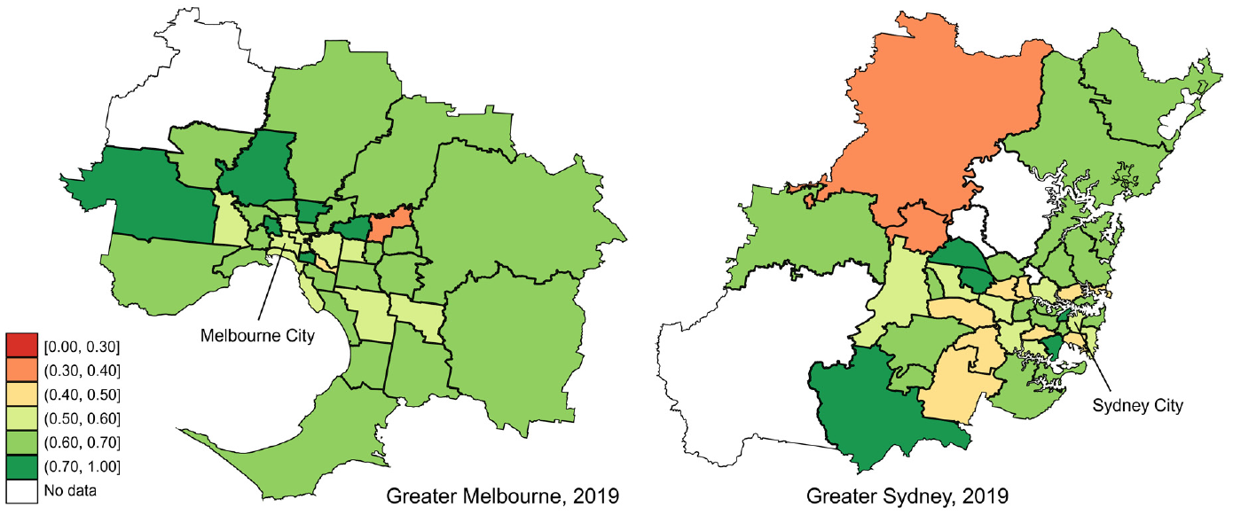
Percentage of middle-income households by SA3 area in Greater Melbourne and Greater Sydney, based on pre-expenditure income, using wave 19 of the HILDA Survey.

Figure 3.

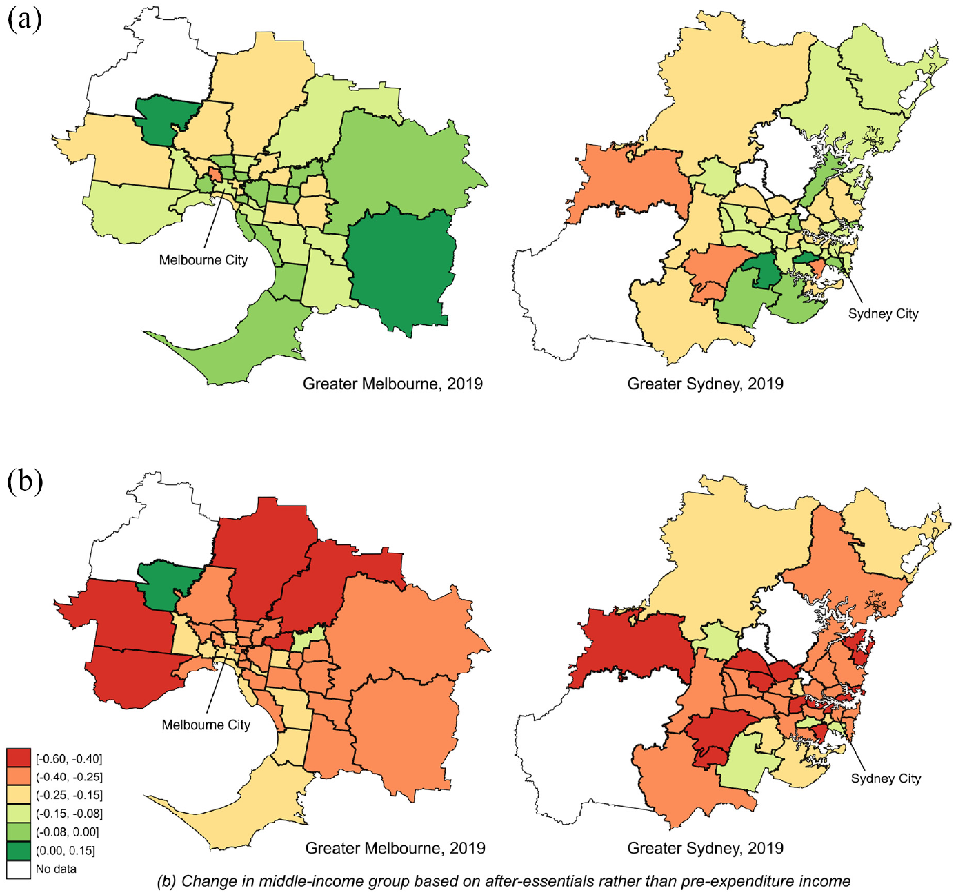
Percentage point change in middle-income households by SA3 area in Greater Melbourne and Greater Sydney, when the percentage based on pre-expenditure income is deducted from the percentage based on expenditure-adjusted income, using wave 19 of the HILDA Survey. (a) Change in middle-income group based on after-housing rather than pre-expenditure income. (b) Change in middle-income group based on after-essentials rather than pre-expenditure income.

In Sydney, middle-income households are much less evenly spread spatially when measured in pre-expenditure income, suggesting a more spatially polarised city compared to Melbourne (Figure 2). The level of spatial polarisation – that is, dissimilarity in the size of the middle-income group across different metropolitan areas – rises further when measured in after-housing income. However, like Melbourne, there is also a decline in middle-income households in the inner suburbs when measured in after-housing income. Again, similar to Melbourne, the proportion of middle-income households declines across the board when measured in after-essentials income (Figure 3).

Discussion

Our analysis found no evidence of significantly increased polarisation in Australia between 2005 and 2019, however the analysis shows the Australian society is a more polarised one – with a smaller middle class – when measured in after-housing and after-essentials rather than pre-expenditure income. These are not merely adjustments on the edges, but rather a substantially transformed social and spatial structure, when examined through the lens of expenditure-adjusted income. In Sydney, in 2019, the overall class structure transforms from the post-industrial ‘egg’ social structure – small higher-income (11.9%) and lower-income (28.3%) and large middle-income (59.8%) groups – in pre-expenditure income, to a structure closer to (although not quite) that of an hourglass, with a significantly reduced middle (36.9%), and significantly increased top (22.0%) and bottom (41.1%) in after-housing income.

The paper adds to existing literature on socio-tenurial polarisation (Bentham, 1986; Hamnett, 1984; Winter and Stone, 1998), showing how patterns of polarisation differ across tenures in complex ways. For outright owners, a significant number of households shift from the low-income to the middle-income group, and from the middle-income to the higher-income categories, when measured in after-housing rather than pre-expenditure income. In contrast, the middle-income group among renters is smaller than other tenures in pre-expenditure income, and even smaller in after-housing income. Mortgaged owners have the largest proportion of middle-income households in pre-expenditure income, but a higher proportion of them ‘slips down’ into the low-income category in after-housing income, even more so than renters.

The paper has also contributed to understanding the spatial patterns of polarisations. Conceptually ‘spatial polarisation’ has often been understood and measured in terms of spatial segregation between low-income and high-income households (Johnston et al., 2016). Our analysis points to another complementary way to conceptualise and measure spatial polarisation, which can help distinguish it from ‘segregation’. Spatial polarisation can also be measured in terms of the spread of middle-income households across the metropolis. While existing literature on the socio-spatial structure of Australian cities tends to focus on concentrations of disadvantage and advantage in different urban areas (Gleeson and Randolph, 2002), our study highlights that in pre-expenditure income, the middle-income group is relatively evenly spatially spread across Melbourne’s metro. However, in expenditure-adjusted income, the middle-income population appears more spatially polarised (i.e. more uneven spread of middle-income households). After-housing income measures show a reduction in the middle-income population in the inner suburbs; and after-essentials income measures moderate this effect but show a reduction in the middle-income population in the outer-suburbs. These patterns are indicative of a spatial trade-off between different types of expenditure. Clearly, additional and more comprehensive research is needed to better understand interactions between different types of expenditure. But overall, our findings demonstrate that uneven expenditure overall increases spatial polarisation.

These results highlight the importance of essential household expenditure, and housing in particular, as drivers of polarisation that are often missed in analyses which focus on total disposable income. This is not to undermine the significance of labour market structures, and associated distribution of income, as a fundamental underpinning of the Australian class structure (Coelli and Borland, 2016; Davidson et al., 2020). However, in Australia – arguably more so than in many parts of Europe and the United States – housing has been a significant driver of social and spatial polarisation processes.

Conclusion

Discourses of polarisation are fuelled by concerns about growing inequality and a hollowed out middle class. The empirical evidence of polarisation is mixed, and our study has demonstrated that different definitions and measures lead to different findings on the extent to which polarisation occurs in practice, and the processes that drive it. We have highlighted the need to account for both income (and underlying labour dynamics) and expenditure (and underlying housing, energy and food market dynamics). The literature on polarisation has acknowledged costs of living as a driver of a shrinking middle class; however, it has overlooked the fact that uneven expenditure can push households not only under, but also above their middle-class position. This is primarily the case for outright owners, or those with relatively low monthly mortgage payments, whose after-housing income ‘rises’ relative to other households. This multiplies the hollowing out effect. Importantly, these processes are inherently spatial, showing distinctive patterns of spatial polarisation for different measures, with significant variation between cities and countries.

Polarisation is a useful concept and a fruitful agenda for future research in urban studies. More nuance is needed in its conceptualisation and measurement, leaving much room for innovation in future research. Some potential directions include the use of more sophisticated categories of class, beyond the blunt instruments of ‘low’, ‘middle’ and ‘high’ income groups used here and in other literature, including intersections with other forms of social diversity such as life-course stage, gender, race, ethnicity, disability etc. There is a need to continue to refine and improve methodologies to study polarisation, including understanding interactions across different expenditure categories, such as childcare that has grown in significance in many household budgets; improved conceptualisation of ‘essential’ expenditure, recognising discretionary spending even within ‘essential expenditure’ categories, and vice versa; and, accounting for wealth, educational attainment, attitudes and behavioural practices and other aspects of social class beyond income. There is also ample scope for qualitative research on the lived experiences of ‘slipping down’ or ‘moving up’ from the middle class through both income and expenditure, and the social relations that characterise urban societies experiencing different forms of polarisation. Our findings open up new directions in the analysis of ‘spatial polarisation’, highlighting that cities can be at once sites of polarisation (measured by clustering of high- and low-income households in different parts of the city), while maintaining a relatively even distribution of the middle class across the metropolitan area. The implications of such a spatial structure require further study.

Footnotes

Acknowledgements

The authors wish to thank the editors and three anonymous reviewers whose valuable comments substantially improved the quality of the paper. This research received in-kind support from the Australian Government through the Australian Research Council’s Centre of Excellence for Children and Families over the Life Course (Project ID CE200100025). This paper uses unit record data from Restricted Release 19 of the Household, Income and Labour Dynamics in Australia (HILDA) Survey. The HILDA Survey is conducted by the Melbourne Institute: Applied Economic & Social Research on behalf of the Australian Government Department of Social Services (DSS). The findings and views reported in this paper are those of the authors and should not be attributed to the Australian Government, DSS or the Melbourne Institute.

Declaration of conflicting interests

The authors have no conflicts of interest to declare.

Funding

The author(s) received no financial support for the research, authorship, and/or publication of this article.

ORCID iDs

Julia de Bruyn

Jordy Meekes

References

ABS (2021) Australian Statistical Geography Standard (ASGS) Edition 3. Australian Bureau of Statistics. Available at: https://www.abs.gov.au/statistics/standards/australian-statistical-geography-standard-asgs-edition-3/latest-release (accessed 1 February 2022).

ACOSS and Brotherhood of St Laurence (2018) Energy Stressed in Australia. Sydney: Australian Council of Social Service (ACOSS). Available at: https://www.bsl.org.au/research/publications/energy-stressed-in-australia/ (accessed 10 February 2022).

Autor

Katz

Kearney

(2006) The polarization of the U.S. labor market. American Economic Review 96(2): 189–194.

Autor

Levy

Murnane

(2003) The skill content of recent technological change: An empirical exploration. The Quarterly Journal of Economics 118(4): 1279–1333.

Babones

(2008) Income inequality and population health: Correlation and causality. Social Science & Medicine 66(7): 1614–1626.

Banerjee

Duflo

(2003) Inequality and growth: What can the data say? Journal of Economic Growth 8(3): 267–299.

Bárcena-Martin

Deutsch

Silber

(2018) On the decomposition of the Foster and Wolfson Bi-polarization index by income sources. Review of Income and Wealth 64(4): 853–871.

Beaulac

Kristjansson

Cummins

(2009) A systematic review of food deserts, 1966-2007. Preventing Chronic Disease 6(3): A105.

Bentham

(1986) Socio-tenurial polarization in the United Kingdom, 1953-83: The income evidence. Urban Studies 23(2): 157–162.

10.

Buzar

(2007) The ‘hidden’ geographies of energy poverty in post-socialism: Between institutions and households. Geoforum 38(2): 224–240.

11.

Carrillo

Castanheira

(2008) Information and strategic political polarisation. The Economic Journal 118(530): 845–874.

12.

Chakravarty

D’Ambrosio

(2010) Polarization orderings of income distributions. Review of Income and Wealth 56(1): 47–64.

13.

Coelli

Borland

(2016) Job polarisation and earnings inequality in Australia. Economic Record 92(296): 1–27.

14.

Davidson

Bradbury

Wong

, et al. (2020) Inequality in Australia, 2020. Part 2: Who is Affected and Why. Sydney, NSW: Australian Council of Social Service (ACOSS) and University of New South Wales (UNSW). Available at: https://apo.org.au/node/310195 (accessed 10 February 2022).

15.

Dinca-Panaitescu

Walks

(2015) Income Inequality, Income Polarization, and Poverty: How Are They Different? How Are They Measured?Toronto, ON: United Way Toronto & York Region and the Neighbourhood Change Research Partnership, University of Toronto.

16.

Dodson

Sipe

(2008) Shocking the suburbs: Urban location, homeownership and oil vulnerability in the Australian city. Housing Studies 23(3): 377–401.

17.

Dollman

Kaplan

La Cava

, et al. (2015) Household economic inequality in Australia. Research Discussion Paper, Reserve Bank of Australia.

18.

Esteban

Ray

(1994) On the measurement of polarization. Econometrica 62(4): 819–851.

19.

Gleeson

Randolph

(2002) Social disadvantage and planning in the Sydney context. Urban Policy and Research 20(1): 101–107.

20.

Goos

Manning

Salomons

(2009) Job polarization in Europe. American Economic Review 99(2): 58–63.

21.

Wang

(2022) Income inequality and global political polarization: The economic origin of political polarization in the world. Journal of Chinese Political Science 27: 375–398.

22.

Hagenaars

de Vos

Zaidi

(1995) Poverty Statistics in the Late 1980s: Research Based on Micro-Data. Luxembourg: Office for Official Publications of the European Communities.

23.

Hamnett

(1984) Housing the two nations: Socio-tenurial polarization in England and Wales, 1961–81. Urban Studies 21(4): 389–405.

24.

Hamnett

(2021) The changing social structure of global cities: Professionalisation, proletarianisation or polarisation. Urban Studies 58(5): 1050–1066.

25.

Holmqvist

Wiesel

(2022) Elite communities and polarization in Neoliberal Society: Consecration in Australia’s and Sweden’s wealthy neighbourhoods. Critical Sociology. Epub ahead of print 7 July 2022. DOI: 10.1177/08969205221108656.

26.

Hulse

Burke

(2000) Social exclusion and the private rental sector: The experiences of three market liberal countries. In: European network for housing research conference, Gavle, Sweden, 26–30 June.

27.

Johnston

Manley

Jones

(2016) Spatial polarization of presidential voting in the United States, 1992–2012: The “Big Sort” revisited. Annals of the American Association of Geographers 106(5): 1047–1062.

28.

Kalb

Meekes

(2021) Wage growth distribution and changes over time: 2001–2018. Australian Economic Review 54(1): 76–93.

29.

Kaufman

MacDonald

Lutz

, et al. (1997) Do the poor pay more for food? Item selection and price differences affect low-income household food costs (Report no. 759). Washington, DC: US Department of Agriculture.

30.

Keister

Southgate

(2022) Inequality: A Contemporary Approach to Race, Class, and Gender. Cambridge: Cambridge University Press.

31.

Mendoza

(2011) Why do the poor pay more? Exploring the poverty penalty concept. Journal of International Development 23(1): 1–28.

32.

OECD (2019) Under Pressure: The Squeezed Middle Class. Paris: OECD Publishing. Available at: https://www.oecd.org/social/under-pressure-the-squeezed-middle-class-689afed1-en.htm (accessed 10 February 2022).

33.

Piketty

(2014) Capital in the Twenty-First Century. Cambridge, MA: Belknap Press.

34.

Ravallion

Chen

(1997) What can new survey data tell us about recent changes in distribution and poverty? The World Bank Economic Review 11(2): 357–382.

35.

Reeves

Guyot

Krause

(2018) Defining the Middle Class: Cash, Credentials, or Culture?Washington, DC: Brookings. Available at: https://www.brookings.edu/research/defining-the-middle-class-cash-credentials-or-culture/ (accessed 15 March 2022).

36.

Rodríguez

(2006) Measuring bipolarization, inequality, welfare and poverty. Working Paper 39. Rome: ECINEQ, Society for the Study of Economic Inequality.

37.

Roope

Niño-Zarazúa

Tarp

(2018) How polarized is the global income distribution? Economics Letters 167: 86–89.

38.

Sassen

(1991) The Global City. Princeton, NJ: Princeton University Press.

39.

Saunders

Naidoo

Wong

(2022) The crumbling pillar: Assessing the impact of housing costs on recent trends in poverty and deprivation in Australia. International Journal of Social Welfare 31(4): 421–432.

40.

Sila

Dugain

(2019) Income, wealth and earnings inequality in Australia. Working Paper No. 1538. Paris: OECD Economics Department.

41.

Smoyer-Tomic

Spence

Amrhein

(2006) Food deserts in the Prairies? Supermarket accessibility and neighborhood need in Edmonton, Canada. The Professional Geographer 58(3): 307–326.

42.

Summerfield

Garrard

Hahn

, et al. (2020) HILDA User Manual - Release 19. University of Melbourne: Melbourne Institute: Applied Economic and Social Research. Available at: https://melbourneinstitute.unimelb.edu.au/__data/assets/pdf_file/0009/3562857/HILDA-User-Manual-Release-19.0.pdf (accessed 10 February 2022).

43.

Torcal

Comellas

(2022) Affective polarisation in times of political instability and conflict. Spain from a comparative perspective. South European Society & Politics 27(1): 1–26.

44.

Weller

van Hulten

(2012) Gentrification and displacement: The effects of a housing crisis on Melbourne’s low-income residents. Urban Policy and Research 30(1): 25–42.

45.