Contextual poverty and obtained educational level and income in Sweden and the Netherlands: A multi-scale and longitudinal study

Abstract

Chinese

Studies of neighbourhood effects typically measure the neighbourhood context at one specific spatial scale. It is increasingly acknowledged, however, that the mechanisms through which the residential context affects individual outcomes may operate at different spatial scales, ranging from the very immediate environment to the metropolitan region. We take a multi-scale approach to investigate the extent to which concentrated poverty in adolescence is related to obtained education level and income later in life, by measuring the residential context as bespoke neighbourhoods at five geographical scales that range from areas encompassing the 200 nearest neighbours to areas that include the 200k+ nearest neighbours. We use individual-level geocoded longitudinal register data from Sweden and the Netherlands to follow 15/16-year-olds until they are 30 years old. The findings show that the contextual effects on education are very similar in both countries. Living in a poor area as a teenager is related to a lower obtained educational level when people are in their late 20s. This relationship, however, is stronger for lower spatial scales. We also find effects of contextual poverty on income in both countries. Overall, this effect is stronger in the Netherlands than in Sweden. Partly, this is related to differences in spatial structure. If only individuals in densely populated areas in Sweden are considered, effects on income are similar across the two countries and income effects are more stable across spatial scales. Overall, we find important evidence that the scalar properties of neighbourhood effects differ across life-course outcomes.

Keywords

bespoke neighbourhoods contextual poverty education income multi-scale neighbourhood effects

Introduction

For a long time, it has been theorised that living in areas of concentrated poverty restricts the opportunities of residents and has a negative effect on individuals’ socio-economic status (Brooks-Gunn et al., 1997; Leventhal and Brooks-Gunn, 2000; McKenzie et al., 1967; Wilson, 1987). Many studies have examined these so-called neighbourhood effects on socio-economic outcomes, including income and educational achievement. Some of these studies focus on adult exposure and adult outcome (Galster et al., 2008; van Ham and Manley, 2010), while other studies investigate adult or youth outcomes in relation to exposure in childhood and adolescence (Andersson and Subramanian, 2006; Andersson et al., 2021; Chetty et al., 2016; Nieuwenhuis et al., 2021; van Ham et al., 2014).

In recent years, many important steps forward have been taken in the field of neighbourhood effects. Scholars moved from point-in-time measures to taking neighbourhood histories of individuals into account (Andersson, 2004; Hedman et al., 2015; Musterd et al., 2012; Sharkey, 2008), found ways to control for non-random neighbourhood selection (Troost et al., 2022; van Ham et al., 2018) and used alternative definitions and operationalisations of neighbourhoods by moving from administrative units to bespoke neighbourhoods in order to circumvent the Modifiable Areal Unit Problem (Hipp and Boessen, 2013; MacAllister et al., 2001; Malmberg et al., 2011).

Another important refinement in the neighbourhood effects literature is the adoption of a multi-scale approach. Neighbourhood effects (also referred to as spatial context effects) are multi-scalar in nature, as different processes play at different spatial scales (Andersson and Malmberg, 2015, 2018; Andersson et al., 2018; Fowler, 2016; Knies et al., 2021; Petrović et al., 2018). Bespoke neighbourhoods are spatially flexible and can be constructed at multiple geographical scales (Johnston et al., 2004). It is now increasingly acknowledged that there is not one correct scale to measure the residential context and that neighbourhood effects must be investigated as a multi-scale phenomenon.

In the current study, we investigate how exposure to contextual poverty at multiple spatial scales in adolescence is related to obtained educational level and income in adulthood. There are several causal mechanisms that can explain how the concentration of poverty in the residential area might be related to socio-economic outcomes later in life such as collective socialisation, social control and cohesion and access to job opportunities (Ainsworth, 2002; Galster, 2012; Sampson, 2012; Wilson, 1987: 198). These mechanisms may operate on different spatial scales (Galster and Sharkey, 2017; Sharkey and Faber, 2014). For example, peer group effects and role model effects can be expected to have an influence at the very low scale, in people’s immediate residential environment. At more intermediate scales, institutional mechanisms and stigma effects can play a role, and at much higher scales, regional labour market effects may influence individual socio-economic outcomes (Andersson and Malmberg, 2015). Despite the fact that there are good theoretical reasons to investigate neighbourhood effects on multiple scales, many empirical studies of neighbourhood effects include the spatial context at just one spatial scale, often using administrative spatial units.

The aim of the current study is to come to a better understanding of the effect of exposure to contextual poverty in adolescence on individual socio-economic outcomes in adulthood. We examined the extent to which contextual poverty concentration is related to obtained educational level and income, over and above family characteristics related to education and income. We took a longitudinal approach, by measuring the concentration of poverty in the residential area at age 15/16 and obtaining educational level and income at age 30. Whereas previous studies were often limited to using relatively large pre-defined administrative areas to measure contextual poverty, we used bespoke neighbourhoods and explicitly took a multi-scale approach. We examined the effect of contextual poverty at five different spatial scales, ranging from very small (i.e. 200 nearest neighbours) to large (i.e. 204,800 nearest neighbours). Finally, we tested the possible generality of these multi-scale effects by comparing Sweden and the Netherlands. It is possible that neighbourhood effects (on educational achievement and income) will differ in countries with different segregation patterns and that have different welfare state regimes (Andersson et al., 2018). We compared patterns of contextual poverty at multiple scales between the two countries and analysed identical models for the effects of contextual poverty experienced in adolescence on obtained education and income for Sweden and the Netherlands.

Theoretical and methodological considerations

Mechanisms at multiple scales

The literature on neighbourhood effects provides strong conceptual support for the idea that neighbourhood effects vary with spatial scale (Andersson and Malmberg, 2015; Andersson and Musterd, 2010; Petrović et al., 2020; van Ham et al., 2012). Based on the idea of multi-scale effects, it has been suggested that it is better to refer to residential context, contextual area effects or residential environment effects, rather than neighbourhood effects, because many effects are likely to play out at different scales than the neighbourhood (Petrović, 2020; Sharkey and Faber, 2014). Conceptually, social and institutional mechanisms related to the spatial context in which one lives are connected to different spatial scales. Having said that, it is not immediately clear from the literature how small or large areas should be in order to influence the outcomes of individual levels of education and income (Friedrichs, 2016). That is, at what levels do relevant social mechanisms operate concerning income and education?

To better understand the different mechanisms at different spatial scales, one could think of influence on education according to age (Andersson and Malmberg, 2015; Maloutas et al., 2019). With increasing age, the daily mobility of an individual increases to include locations which are further and further away. The literature on children’s and adolescents’ mobility (van der Burgt, 2008) considers pre-school children and their mobility with parents to and from pre-school, and the close-to-home outdoor activities and contacts they make with other pre-school children and neighbouring children. The size of the area and thereby the nearby population that pre-school children reach within a day is much smaller than that for an adolescent of 15 or 16 years of age. The latter age group, which is the cohort of this study, moves around urban areas more independently, and is therefore potentially exposed to very large geographical areas and their populations due to school locations and out-of-school activities (Barthon and Monfroy, 2010). Conceptually, the ideas about geographical reach, taking into account modes of travel, are connected to the time-geography approach (Hägerstrand, 1970). The basic ideas of time-geography include that children will be more influenced by nearby environments than by more distant or far away surroundings, and that their modes of transportation are limited, which gives them a short spatial reach for daily activities. Thus contextual influence on children and adolescents might be local and then span suburbs and parts of cities as they age. There are capability constraints that limit travel distance when spending the night in the same home, as well as authority constraints in cost to enter certain domains and coupling constraints when individuals and things have to be coordinated in time and place (Andersson et al., 2012).

The literature on residential context effects also provides some ideas of the different spatial scales which are relevant for the understanding of the two outcome variables for this study: education and income. For educational achievements, the surrounding peers’ parents are important as role models (Ainsworth, 2002), for example through their educational level and through social control in monitoring homework and help in studying. There are also likely to be direct peer effects through educational attitudes towards being ‘good in school’, that is, being brought up in the spirit that education is the most important thing for success in later life. These effects we expect to be local in character, including the closest peers; for example, 200. In addition, the influence on adolescents’ education will also run through the quality of local institutions like the school (Kuyvenhoven and Boterman, 2021; Owens and Candipan, 2019). Here, the relevant scale (population to reach) would be the size of the school population (Andersson et al., 2021).

For later in life income, the neighbouring peers’ parents are equally important in role modelling. These role models can show non-employment careers or employment careers at different socio-economic levels. Visible signs in the neighbourhood such as decay or affluence are another issue that was much discussed in terms of social disorganisation in the earlier literature (Sampson, 2012; Wilson, 1987). Individual income can also be expected to be influenced by the larger regional context in which adolescents grow up; for example, by regional employment structures in terms of levels of (un)employment, and the broader occupational structure of regional labour markets (Andersson and Malmberg, 2015; Kristiansen et al., 2022). An effect on future income was found for high unemployment levels at k = 12,800. That is, income can be considered somewhat less directly influenced compared to education (Andersson and Musterd, 2010). The assumed influence on level of income is rather through the labour market structure. We studied the residential context at age 15/16 and earlier, and considered that socialisation mechanisms, including role models, norms, social control and peer groups, are most important at that age. We therefore expected to find stronger contextual effects of poverty at the smaller spatial scale than at the larger spatial scale.

Cross-national comparison: Sweden and the Netherlands

There are two main reasons why a cross-national comparison is fruitful for residential context effects research. First, contextual effects of poverty on educational attainment and income level can differ between countries as segregation levels and patterns in turn are different. Second, these contextual effects can also differ between countries that have different welfare state regimes. Even when poverty levels and spatial patterns of poverty are similar between countries, the magnitude of residential context effects can differ according to the welfare system. One system might compensate for negative context effects more strongly than the other. The fact that Korpi and Palme (1998) label Sweden as having an encompassing welfare model, and label the Netherlands as having a basic security welfare model, could be of importance here. Esping-Andersen (1999), on the other hand, classifies the two countries as belonging to the same universalist welfare state regime, something that is also reflected in the redistributive budget size and income redistribution of Sweden and the Netherlands, as reported by Korpi and Palme (1998). Thus, at this stage, it is not clear how variation in welfare state arrangements between Sweden and the Netherlands can be expected to have consequences for the differences in how residential contexts influence individual-level outcomes between the two countries. (For extensive reading of country and city comparisons, see Haandrikman et al., 2021; Musterd, 2005; van Ham et al., 2021.)

Bespoke neighbourhoods

Especially when doing cross-national studies of contextual effects, it is important to carefully choose the same and specific geographical scale for the analyses, as using different scales can affect the outcomes of the comparison (Andersson and Malmberg, 2015; Andersson and Musterd, 2010; Andersson et al., 2018: 201). Large-scale geographic areas hide homogenous pockets of poverty concentration, whereas areas which are too small can overstate contextual poverty concentration as small areas often are more homogenous. Thus, the degree of poverty concentration cannot be compared between countries if one has systematically differently sized areas (Andersson et al., 2018). In recent years, the increasing availability of individual-level geocoded data has led scholars from different fields to use bespoke neighbourhoods to measure spatial contexts. Different terms are used to label bespoke neighbourhoods, including individualised neighbourhoods, scalable neighbourhoods, egocentric neighbourhoods, egocentric buffers, egohoods, overlapping neighbourhoods and individual social environments (Hipp and Boessen, 2013; MacAllister et al., 2001; Malmberg et al., 2011).

A method to create such bespoke neighbourhoods determines neighbourhoods based on a predetermined equal number of nearest neighbours (e.g. Malmberg et al., 2011; Östh et al., 2015). This k-nearest neighbours approach results in areas of different sizes without fixed borders, but with fixed population counts. Using equal population counts avoids the risk that measures of contextual poverty in areas with low population density will be inflated by random variance in population composition, or will be based on data from very few individuals or households (Östh et al., 2015). These bespoke measures are more spatially flexible when built up from very small spatial units (such as individual addresses, or 100 × 100-metre grid cells). In order to investigate the extent to which poverty concentration at multiple geographical scales in the adolescent residential area is persistently related to educational achievement and income later in life, we need data that (1) covers the whole population, (2) is longitudinal, (3) provides information on income and (4) is geocoded at a small spatial scale. This type of data is available in both Sweden and the Netherlands.

The k-nearest neighbours method provides standardised measures of contextual poverty as it uses equal population counts, which makes it easier to compare results across countries with different geographies and spatial distributions of the population, such as Sweden and the Netherlands. Especially at higher spatial scales, the area needed to reach a given k-nearest neighbour will be much larger in Sweden than in the Netherlands. This has theoretical implications, as the chance of meeting and interacting with your k-nearest neighbours in a smaller geographical area is greater than in a larger geographical area. This also makes it interesting to compare these two countries on the effects of the poverty concentration on socio-economic outcomes.

Data and methods

Data

Data for this study come from national population register data from the Netherlands and Sweden. For the Nether-lands, the data source is the Social Statistical Database (SSD, or Social Statistisch Bestand (SSB)) (Bakker, 2002; Houbiers, 2004). The SSD data cover the entire population of the Netherlands since 1999 and contain data from a range of government registers, including population, tax and housing registers. The data are geocoded at the level of 100 × 100 m grids for the whole country. The data for Sweden originate from Statistics Sweden’s registers in a project called Migrant Trajectories covering the years 1990–2016. Data are accessed through an online system called MONA (Statistics Sweden, 2018). The Swedish data are geocoded at the level of 250 × 250 m grid cells in urban areas (defined as localities consisting of a group of buildings normally not more than 200 m apart from each other, and with at least 200 inhabitants), and 1000 m squares outside these urban areas, based on the 2010 urban subdivision. The urban and rural grids are positioned in such a way that 16 urban grid cells can fit into one rural grid cell (see Nielsen et al., 2017: 24–25).

Sample

For the Netherlands, we studied the 1987 birth cohort (n = 144,698; see Table 1). These individuals were 30 years old in 2017, the last year for which register income data were available at the time this study was conducted. We included neighbourhood characteristics from the year 2003, when these individuals were 16 years old. For Sweden, we studied the 1986 cohort (n = 101,687). Residential context was measured for the year 2001, when the cohort was 15 years of age. Since exposure time during adolescence is important for an assessment of later effects on outcomes, we selected individuals who lived for at least three subsequent years in the same grid cell.

Table 1.

Descriptive statistics of individual and contextual characteristics in the Netherlands and Sweden.

	The Netherlands				Sweden
Variable	Mean	SD	Min	Max	Mean	SD	Min	Max
Individual characteristics
Obtained educational level (years)	15.97	1.89	2	22	13.00	2.21	6	20
Income age 30 (percentiles)	70.28	22.25	1.00	100.00	67.76	24.80	4.66	100
Male	51%				51%
Non-European migration background	13%				8%
Family characteristics
Single-parent^a family (age 15/16)	13%				22%
Social allowance (age 15/16)	4%				7%
Tertiary education parents
No parents with tertiary education	42%				60%
One parent	15%				26%
Two parents	3%				15%
Missing	40%				–
Equalised disposable household income (age 15/16; thousand Euros)	21.05	13.57	–^b	–^b	10.3	14.4	0	2809.0
Unemployment parents (age 15/16)
No unemployed parents	69%				58%
One parent	27%				33%
Two parents	4%				9%
Contextual characteristics
Poverty rate k = 200	0.09	0.06	0	0.90	0.08	0.06	0.00	0.75
Poverty rate k = 1600	0.09	0.04	0.01	0.41	0.08	0.04	0.01	0.73
Poverty rate k = 12,800	0.09	0.03	0.03	0.33	0.08	0.03	0.04	0.40
Poverty rate k = 51,200	0.10	0.03	0.05	0.26	0.08	0.02	0.05	0.25
Poverty rate k = 204,800	0.10	0.02	0.06	0.21	0.09	0.01	0.06	0.14
N _individual	144,698				101,687
N _contextual	103,855				52,637

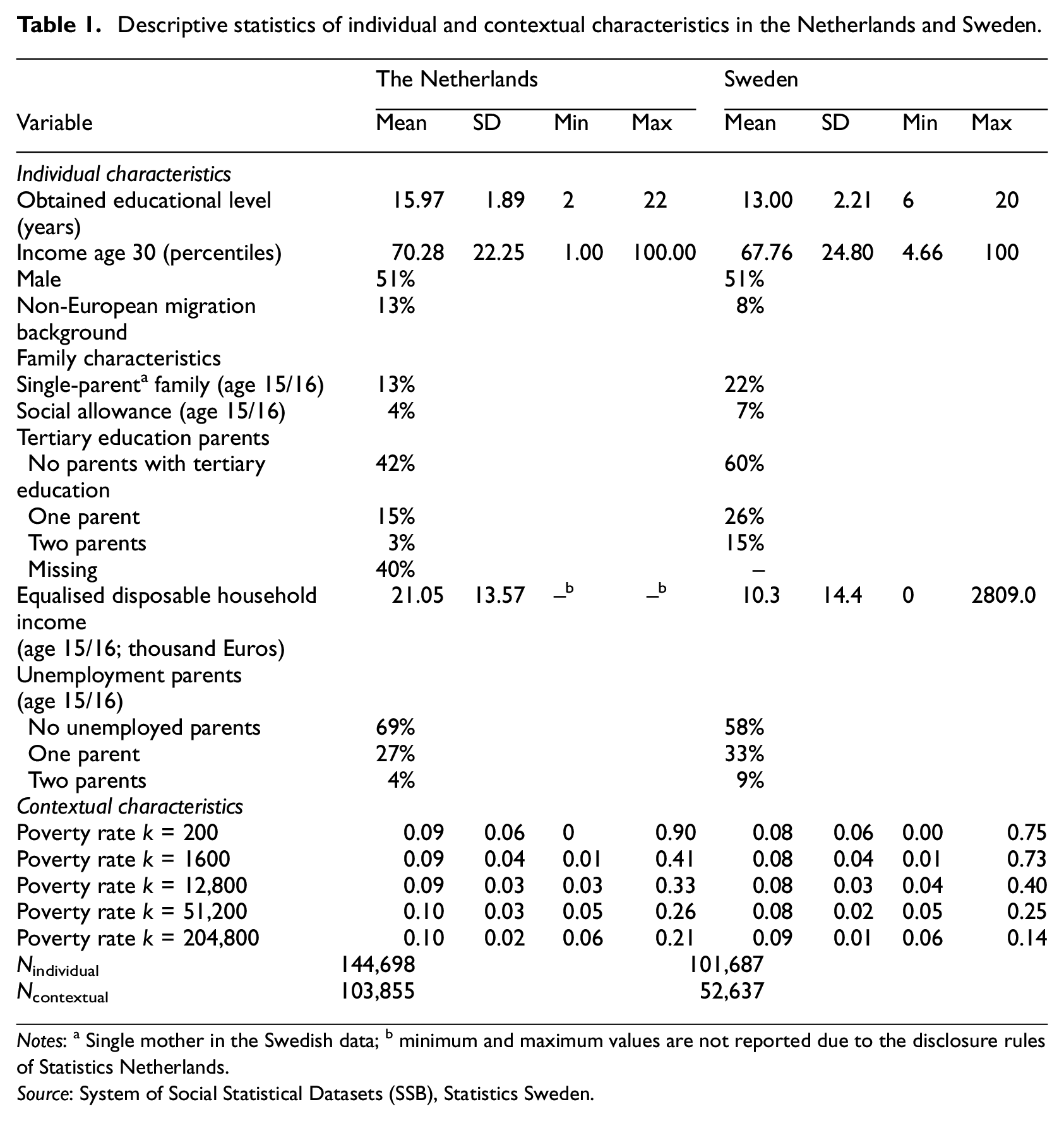
Notes: ^a Single mother in the Swedish data; ^b minimum and maximum values are not reported due to the disclosure rules of Statistics Netherlands.

Source: System of Social Statistical Datasets (SSB), Statistics Sweden.

Obtained education level and income (age 30)

We used two individual outcome variables: obtained educational level and individual earned income at age 30.

Educational level is measured in years. The Netherlands has a highly stratified educational system in which choices regarding the level of study are made as early as age 12. Children attend primary school from the age of four to 12. In their final year, based on a national test and the teacher’s recommendations, they are advised which type of secondary education they should pursue. There are three types of secondary education. One option is lower vocational training (four years), which gives access to intermediate vocational training (one year) at the upper secondary level. The other options are secondary general education (five years) and pre-university education (six years). Only the pre-university track gives direct access to university (four to six years). All three tracks give access to universities of applied sciences (four years). In order to make the Netherlands data comparable to the Swedish data, we converted the obtained educational level to years of education. Sweden has an encompassing and unitary school system. Children are not stratified as in the Dutch system but there are nevertheless choices to be made within the compulsory school, such as language classes. The unified and compulsory school lasts until students are 15 years of age, that is until they complete ninth grade. The grades from the compulsory nine years of school are used to apply for programmes in upper secondary school. Upper secondary school consists of three-year vocational or theoretical programmes, of which the theoretical programmes prepare students for the university programmes, which last over two years. At university level, a bachelor can be obtained with three years of study and a masters education after an additional two years (a total of 17 years). All the educational levels are converted into years to be comparable to the Netherlands, as written above.

Individual earned income (gross) at age 30 is measured in percentiles in order to facilitate comparison of the results between the Netherlands and Sweden. These range from 1 to 100, indicating to what income percentile the individual belongs, and therefore the relative income position within the cohort. As income can fluctuate, especially around age 30, for example due to having children, we calculated the highest income percentile between age 25 and 30 for every individual. Note also that further income differentiation will occur later in life between individuals with different education levels.

Individual and family characteristics (age 15/16)

As individual-level predictors of income, we included sex (with female as the reference category), and a non-European migration background, which indicated whether at least one parent was born outside of Europe. We included a set of family and parental characteristics when the individual was 15/16 years of age as predictors of individual income and educational level. We included a dummy variable that indicated whether the individual was living in a single-parent household (single-mother household in Sweden). Another dummy variable indicated whether the family received a social allowance. Household income in thousand Euros was included as a continuous variable. Parental tertiary education was included as a categorical variable, with three categories indicating whether no, one or both parent(s) had tertiary education. Parental unemployment was also included as a categorical variable, with three categories indicating whether no, one or both parent(s) were unemployed.

Contextual at-risk-of-poverty rate at multiple spatial scales (age 15/16)

The contextual at-risk-of-poverty rate is measured in a similar way in both countries and is based on the population of individuals aged 25 or older. It is based on the Eurostat definition of the at-risk-of-poverty rate, which is defined as the share of people with an equivalised disposable household income below the at-risk-of-poverty threshold, which is set at 60% of the national median equivalised disposable income (Eurostat, 2018).

We calculated bespoke measures of contextual poverty at multiple geographical scales using EquiPop, a software programme for the calculation of the k-nearest neighbours, developed by Östh at Uppsala University (http://equipop.kultgeog.uu.se). By applying this approach, difference in grid cell size will in most cases not be important, since reaching the target population requires that many grid cells have to be aggregated. The computation of measures of spatial inequality is based on individualised scalable neighbourhoods, based on fixed population counts. We constructed measures of contextual poverty at five different spatial scales, that is, the nearest 200, 1600, 12,800, 51,200 and 204,800 neighbours.

Analytical approach

First, we analysed the patterns of the concentration of at-risk-of-poverty households at multiple geographical scales. In order to compare concentrations of poverty across countries, we followed the approach of Andersson et al. (2018) and present percentile plots of these concentrations at different scales.

Second, we estimated two series of identical linear regression models predicting obtained educational level and income at age 30 in both countries. In Model 1, we only included lagged effects of individual and family characteristics at age 15/16. Here, we used a formal test (z-test) for comparing the coefficients between Sweden and the Netherlands, (Paternoster et al., 1998).¹ In the next set of models, we added lagged effects of the contextual at-risk-of-poverty rate at the five different geographical scales (Models 2a). Individual and family characteristics were included in these models as control variables. It is known that certain types of households sort into certain types of neighbourhoods (van Ham et al., 2018) and that this selective residential mobility is more likely to take place at a smaller geographical scale (van der Meer and Tolsma, 2014). Although we could not fully control for selective sorting, we included variables that were related both to the type of area where the family lived when the individual was a teenager and to the obtained educational level and income of the child later in life. It is possible that the effects of neighbourhood composition are mediated by neighbourhood schools (Hermansen et al., 2020), but investigating this is beyond the scope of this article.

The distance that has to be covered from a particular grid cell to reach a targeted population depends on the population density. In sparsely populated areas in Sweden, the buffer has to reach wider to encompass the same number of k-nearest neighbours compared to the Netherlands. For example, in the Netherlands, a distance of 412 m on average was enough to capture 1600 nearest neighbours at percentile 50, whereas 750 m was needed to enclose 1600 nearest neighbours in Sweden at the same percentile. For a larger number of neighbours, 51,200 individuals, the buffered distance for the Netherlands was almost 5 km but for Sweden it was up to 16 km at the 50th percentile of the total population (see comparisons in Andersson et al., 2018). Thus, overall, the radius of the buffer to enclose k-nearest neighbours is larger in Sweden than in the Netherlands, which reflects the lower population density in Sweden. Because of these differences, we included this distance in a second set of regression models as a control variable (Models 2b).

In a final step, we have re-estimated Swedish models using only observations from more densely populated areas. The cut-off point selected for less densely populated areas was that a radius greater than 330 km was needed in order to reach the highest population threshold, k = 204,800. This corresponds to a 99th percentile value for distance to the nearest 204,800 neighbours in the Netherlands.

Results

Multi-scale patterns of inequality in Sweden and the Netherlands

Figure 1 shows percentile plots for the proportion of households at risk of poverty (i.e. disposable equivalised disposable household income less than 60% of the national median) for bespoke spatial contexts using different k-levels (i.e. 200, 12,800, 204,800). These percentiles show the proportion of the population that is exposed to certain poverty levels in their residential area across countries and k-values (scales). The plots demonstrate that the at-risk-of-poverty population is segregated, that segregation is more present at a low spatial scale and that these patterns are very similar in Sweden and the Netherlands; in fact, the patterns are strikingly similar. Most areas have relatively low proportions of at-risk-of-poverty households, but in a small number of areas the concentration of at-risk-of-poverty households is very high (second column of graphs). For example, the graphs for the lowest spatial scale (k = 200) show that 80% of all neighbourhoods have modest at-risk-of-poverty rates, ranging between 0% and 12% in Sweden and 0% and 14% in the Netherlands. The other 20% of all neighbourhoods have larger proportions of at-risk-of-poverty households, ranging from 12% to 76% in Sweden and 14% to 95% in the Netherlands. In both countries, high proportions of at-risk-of-poverty households are concentrated in a small number of neighbourhoods. One exception to these striking similarities regarding patterns is the larger concentration of poverty in the Netherlands at the largest scales, k = 204,800.

Figure 1.

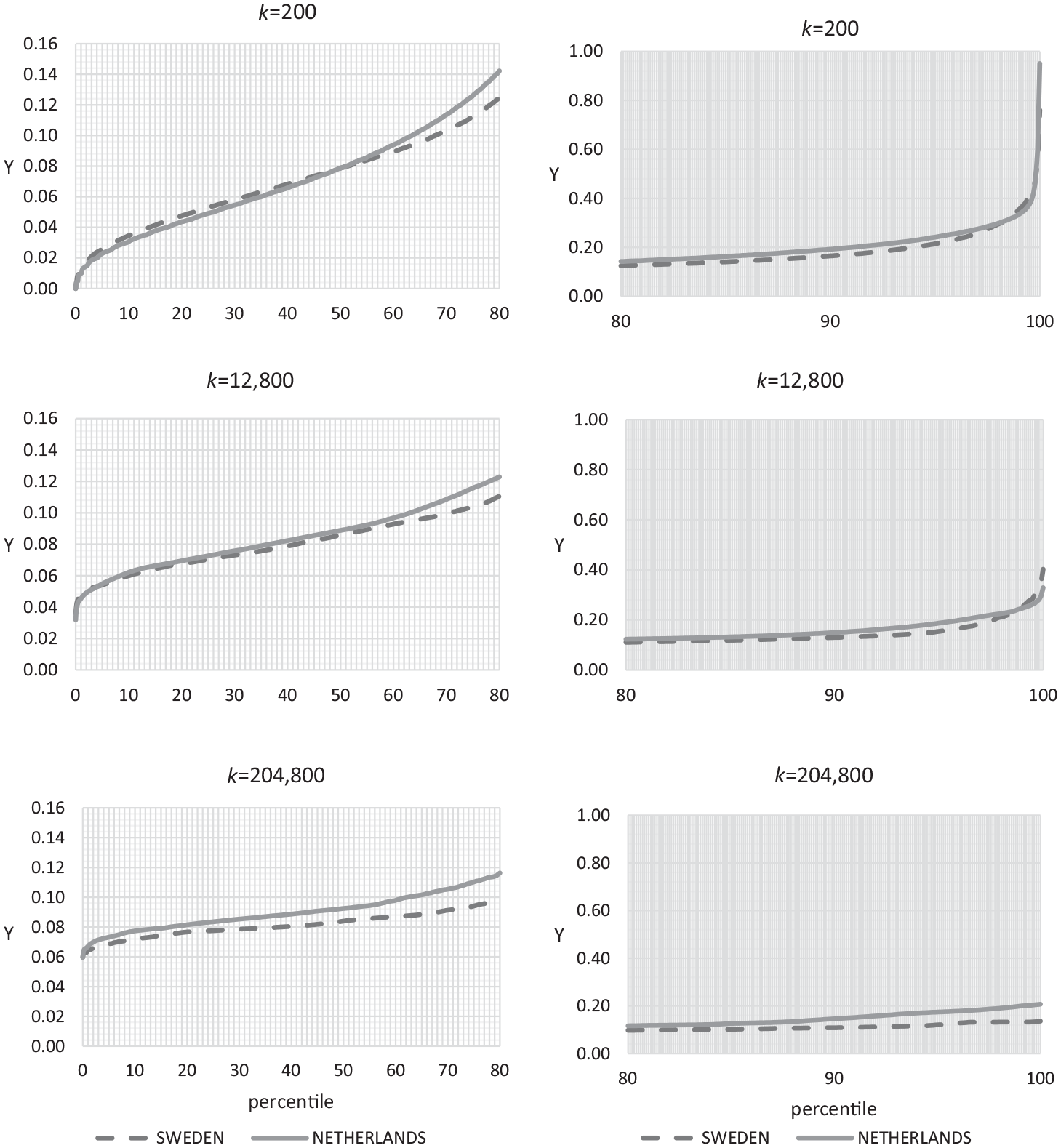
Proportion of households at risk of poverty (y-axis) in bespoke neighbourhoods in Sweden and the Netherlands. Percentiles (x-axis) for different k-values. Lower percentiles (<80) in the first column and higher percentiles (>80) in the second column.

Individual and family characteristics (age 15/16) as predictors of educational level and income (age 30)

First, we present the results of the longitudinal models predicting educational level and income at age 30 with only individual and family characteristics at age 15/16 (Table 2). In both countries, males have a higher income than females. In contrast, males are less highly educated than females. The latter effect, of having lower education due to being male, is slightly stronger in Sweden (z = 10.056, z being the normal deviate test). Individuals with a non-European background are more highly educated but have a lower income.

Table 2.

Obtained educational level (years) and individual earnings (percentile) at age 30 predicted by individual and family characteristics (age 15/16) in the Netherlands and Sweden (Model 1), z-scores for difference Netherlands and Sweden.

	Educational level age 30					Individual earnings age 30
	The Netherlands		Sweden			The Netherlands		Sweden
	B	SE	B	SE	z-Scores	B	SE	B	SE	z-Scores
Male	–0.495^***	0.009	–0.654^***	0.013	10.056^***	9.254^***	0.112	9.473^***	0.151	–1.165
Non-European migration background	0.103^***	0.015	0.227^***	0.024	–4.381^***	–4.897^***	0.175	–0.450	0.289	–13.162^***
Single-parent family (age 15/16)	–0.340^***	0.015	–0.024	0.019	–13.054^***	–3.711^***	0.179	–0.835^***	0.231	–9.841^***
Social allowance (age 15/16)	–0.233^***	0.030	–0.814^***	0.028	14.158^***	–2.606^***	0.359	–6.118^***	0.330	7.202^***
Tertiary education parents (ref. = 0)
One parent	0.927^***	0.014	1.062^***	0.015	–6.579^***	3.622^***	0.170	1.633^***	0.179	8.057^***
Two parents	1.310^***	0.028	1.837^***	0.019	–15.574^***	4.091^***	0.328	1.377^***	0.229	6.784^***
Missing	0.392^***	0.011				2.856^***	0.127
Household income (age 15/16; thousand Euros)	0.012^***	0.000	0.003^***	0.000	63.640^***	0.130^***	0.004	0.027^***	0.005	16.086^***
Unemployment parents (age 15/16; ref. = 0)
One parent	–0.253^***	0.011	–0.344^***	0.017	4.494^***	–2.324^***	0.131	–4.042^***	0.205	7.062^***
Two parents	–0.525^***	0.028	–0.645^***	0.028	3.030^**	–5.006^***	0.326	–8.272^***	0.335	6.987^***
Constant	15.749^***	0.013	12.974^***	0.013		63.041^***	0.149	64.721^***	0.158
Adjusted R²	0.091		0.173			0.084		0.064

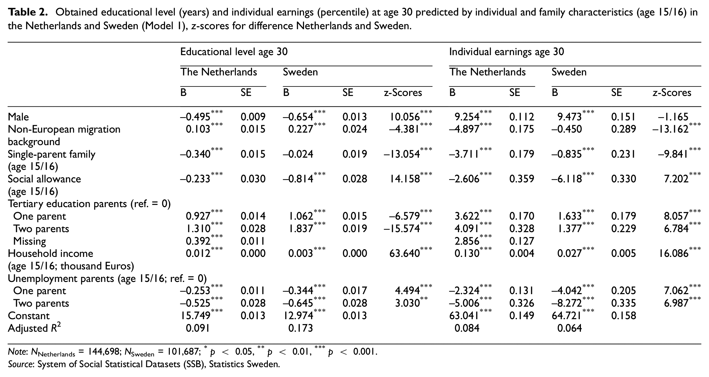
Note: N_Netherlands = 144,698; N_Sweden = 101,687; ^*p < 0.05, ^**p < 0.01, ^***p < 0.001.

Source: System of Social Statistical Datasets (SSB), Statistics Sweden.

The effects of the variables that present the socio-economic status of the family when the individual was 16 years old are all significantly different between Sweden and the Netherlands. Individuals who had a single parent at age 15/16 had a lower educational level and income at age 30, compared to individuals who had a two-parent family. For both education and income, this single-parent effect is stronger in the Netherlands than it is in Sweden (z = −13.054; z = −9.841).

However, having a family on social allowance or unemployed parents at age 15/16 has a stronger negative impact in Sweden than in the Netherlands for both educational outcome and income. For educational achievements, the positive effect of having one or two parents with tertiary education is stronger in Sweden (z = −6.579; z = −15.574), whereas the effect of having tertiary educated parents on income at age 30 is stronger in the Netherlands. A positive effect was also found for household income at age 15/16 on both education level and income at age 30, and this effect is stronger in the Netherlands (z = 63.640) compared to Sweden (z = 16.086).

In total, these individual and family characteristics explained 9.1% of the variance in educational level in the Netherlands and 17.3% in Sweden. The variance explained regarding income in adulthood is 8.4% in the Netherlands and differs from the 6.4% in Sweden.

Multi-scale contextual poverty (age 15/16) as a predictor of educational level and income (age 30)

In Table 3, results are presented from the models that estimated the association between the contextual at-risk-of-poverty rate at age 15/16 and obtained educational level at age 30 in Sweden and the Netherlands. All individual and family characteristics that were included in Model 1 (Table 2) were also included in the models of Table 3, but are not reported.

Table 3.

Educational level (years) at age 30 predicted by contextual poverty (ratios) at age 15/16 at multiple geographical scales in the Netherlands and Sweden.

	Educational level age 30
	The Netherlands					Sweden
	Model 1a			Model 1b				Model 1a	Model 1b		Model 1a (restricted)
					(incl. distance)				(incl. distance)		n = 33,043
	B	SE	Beta	B	SE	B	SE	Beta	B	SE	B	SE	Beta
k = 200
Contextual poverty rate	–2.415^***	0.082	–0.081^***	–2.702^***	0.084	–1.893^***	0.095	–0.063^***	–1.871^***	0.098	–1.914^***	0.142	–0.081^***
Distance				0.028^***	0.002				0	0
Adjusted R²	0.096			0.098		0.176			0.176		0.193
k = 1600
Contextual poverty rate	–2.791^***	0.108	–0.071^***	–2.948^***	0.109	–2.108^***	0.117	–0.056^***	–2.045^***	0.119	–2.111^***	0.159	–0.077^***
Distance				0.007^***	0.001				–0.000^**	0
Adjusted R²	0.095			0.096		0.176			0.176		0.193
k = 12,800
Contextual poverty rate	–2.053^***	0.138	–0.040^***	–2.055^***	0.138	–2.079^***	0.169	–0.037^***	–1.986^***	0.17	–2.059^***	0.22	–0.052^***
Distance				0.002^***	0				–0.000^***	0
Adjusted R²	0.092			0.092		0.174			0.175		0.19
k = 51,200
Contextual poverty rate	–0.943^***	0.161	–0.016^***	–0.862^***	0.162	–2.025^***	0.234	–0.025^***	–2.084^***	0.234	–1.991^***	0.296	–0.035^***
Distance				0.001^***	0				–0.000^***	0
Adjusted R²	0.091			0.091		0.174			0.174		0.189
k = 204,800
Contextual poverty rate	–0.022	0.198	0	0.102	0.201	–1.450^***	0.42	–0.010^***	–2.051^***	0.473	–1.881^**	0.62	–.015^**
Distance				0.000^***	0				–0.000^**	0
Adjusted R²	0.091			0.091		0.173			0.173		0.188

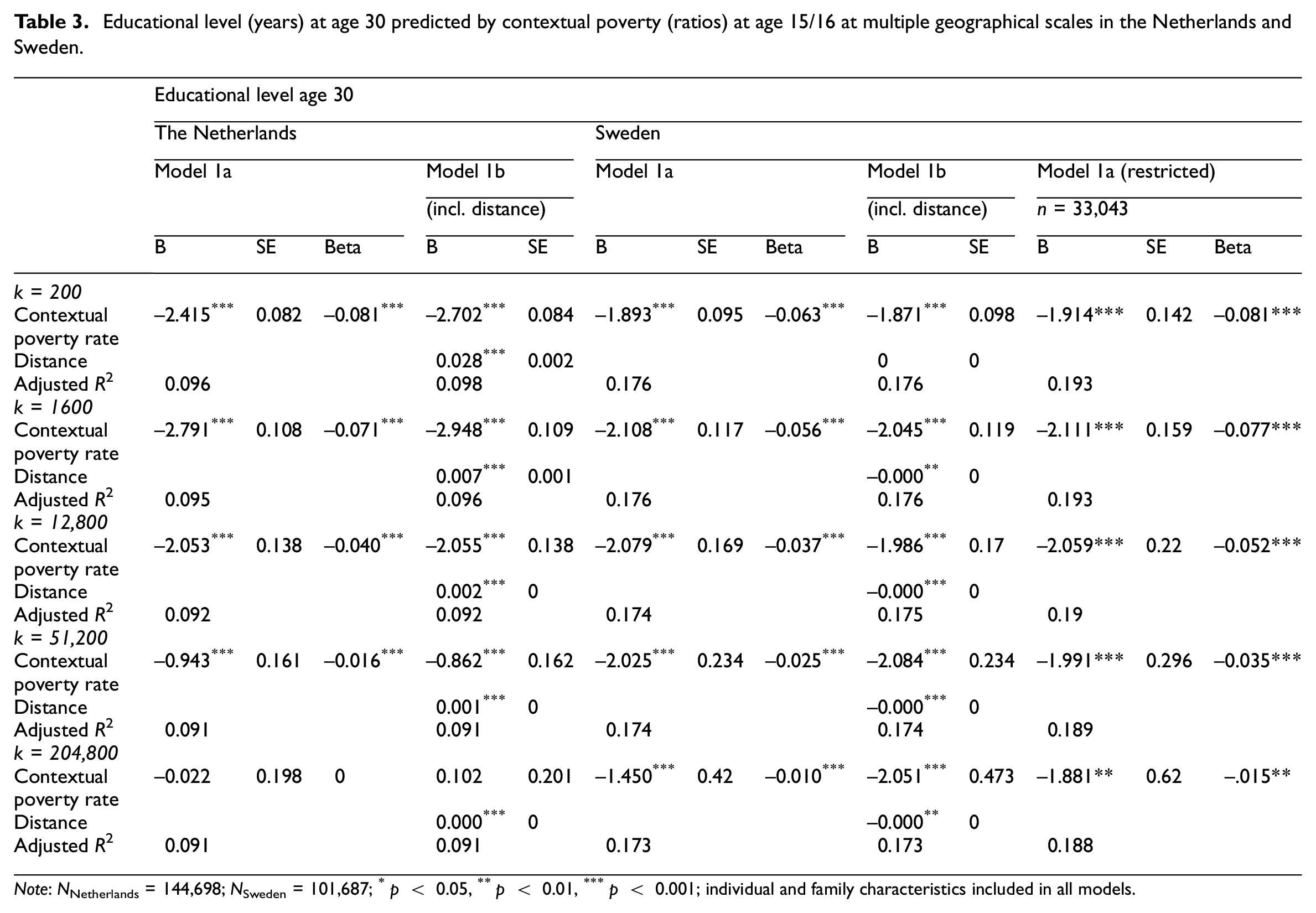
Note: N_Netherlands = 144,698; N_Sweden = 101,687; ^*p < 0.05, ^**p < 0.01, ^***p < 0.001; individual and family characteristics included in all models.

Source: System of Social Statistical Datasets (SSB), Statistics Sweden.

In both countries, the contextual at-risk-of-poverty rate is clearly related to a lower obtained educational level at age 30. The size of the effect, however, decreases with increasing spatial scale. Contextual poverty at a lower spatial scale, among the neighbours that are closest to an individual, has stronger negative consequences for obtained educational level than the at-risk-of-poverty rate at a higher spatial scale. The results show that the effect of contextual poverty at a low spatial scale is stronger in the Netherlands compared to Sweden. At a high spatial scale, the effect is stronger in Sweden and is even non-significant in the Netherlands.

Table 4 presents the models that estimated the relations between the contextual at-risk-of-poverty rate at age 15/16 at multiple spatial scales and individual income at age 30. Similar to the contextual effects we found for educational level, we found that the contextual at-risk-of-poverty rate is also negatively related to obtained income. However, the contextual effects on income show a different pattern from those on educational level. Whereas the contextual effect of the at-risk-of-poverty rate in Sweden again decreases with increasing spatial scale, the contextual effect for the Netherlands does not change much across scales. The results show that at all spatial scales, except the largest spatial scale (k = 204,800), the contextual effect of the at-risk-of-poverty rate on individual income later in life is significantly stronger in the Netherlands than in Sweden.

Table 4.

Individual earnings (percentile) at age 30 predicted by contextual poverty (ratios) at age 15/16 at multiple geographical scales in the Netherlands and Sweden.

	Individual earnings age 30
	The Netherlands					Sweden					Sweden
	Model 2a			Model 2b		Model 2a			Model 2b		Model 2a (restricted)
				(incl. distance)					(incl. distance)		n = 33,043
	B	SE	Beta	B	SE	B	SE	Beta	B	SE	B	SE	Beta
k = 200
Contextual poverty rate	–23.481^***	0.971	–0.067^***	–27.514^***	0.99	–11.703^***	1.138	–0.035^***	–12.707^***	1.17	–16.266^***	1.709	–0.062^***
Distance				0.396^***	0.019				0.000^***	0
Adjusted R²	0.088			0.09		0.065			0.065		0.053
k = 1600
Contextual poverty rate	–35.808^***	1.275	–0.078^***	–38.021^***	1.285	–14.636^***	1.394	–0.035^***	–15.287^***	1.42	–19.289^***	1.92	–0.064^***
Distance				0.102^***	0.007				0.000^*	0
Adjusted R²	0.089			0.09		0.065			0.065		0.054
k = 12,800
Contextual poverty rate	–46.404^***	1.629	–0.077^***	–46.441^***	1.628	–12.408^***	2.015	–0.020^***	–12.387^***	2.026	–21.469^***	2.644	–0.048^***
Distance				0.023^***	0.003				0	0
Adjusted R²	0.089			0.09		0.064			0.064		0.053
k = 51,200
Contextual poverty rate	–51.108^***	1.903	–0.072^***	–51.534^***	1.916	–12.643^***	2.789	–0.014^***	–13.391^***	2.793	–25.537^***	3.566	–0.041^***
Distance				–0.003^*	0.002				–0.000^***	0
Adjusted R²	0.089			0.089		0.064			0.064		0.052
k = 204,800
Contextual poverty rate	–48.465^***	2.342	–0.055^***	–54.067^***	2.378	–13.889^**	5.014	–0.008^**	–44.088^***	5.638	–55.672^***	7.45	–0.041^***
Distance				–0.012^***	0.001				–0.000^***	0
Adjusted R²	0.087			0.088		0.064			0.065		0.052

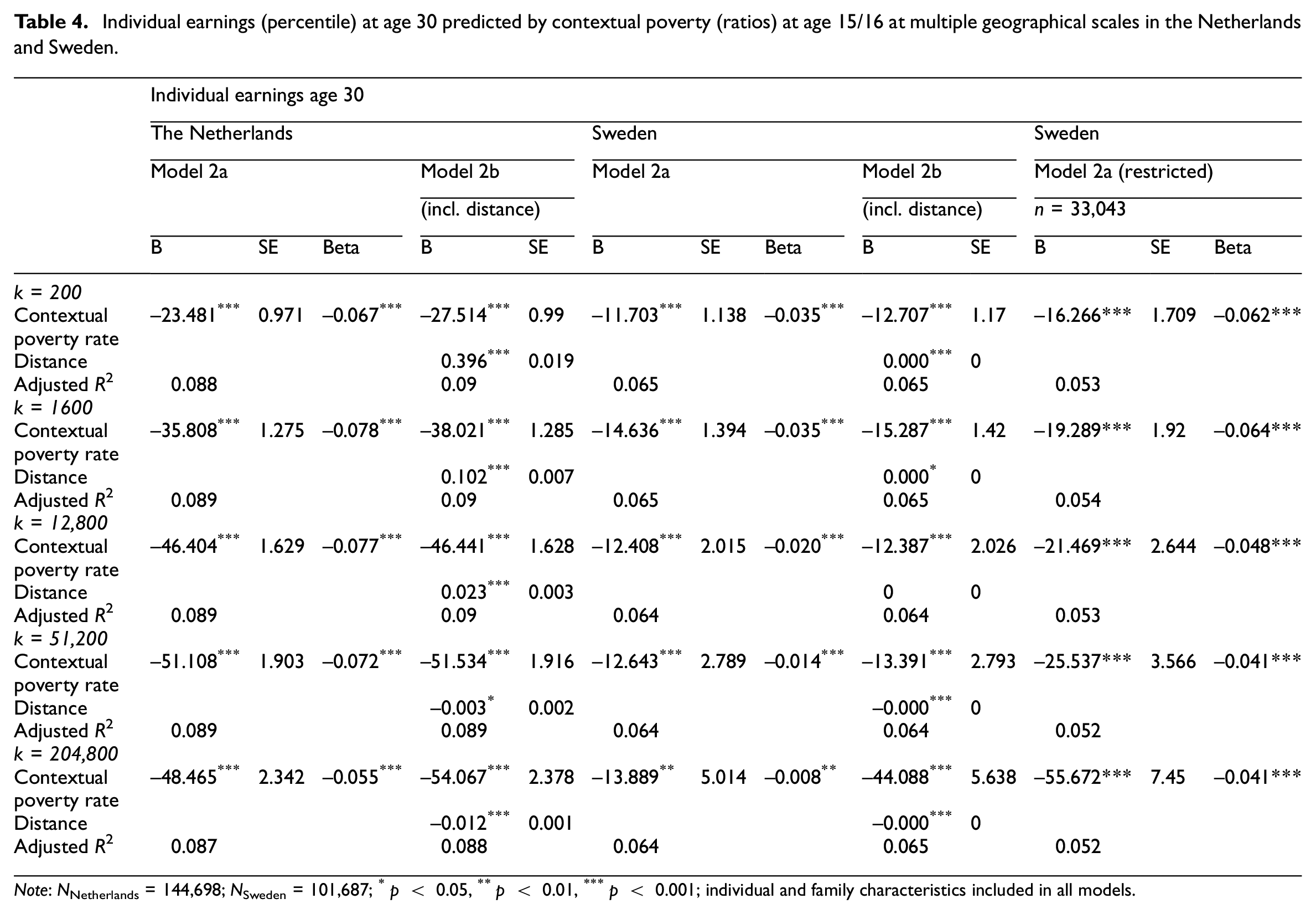
Note: N_Netherlands = 144,698; N_Sweden = 101,687; ^*p < 0.05, ^**p < 0.01, ^***p < 0.001; individual and family characteristics included in all models.

Source: System of Social Statistical Datasets (SSB), Statistics Sweden.

Including distance needed to reach the k-nearest neighbour in the model does not qualitatively change the estimated contextual effects on income (Model 2b). However, if individuals living in less densely populated areas are excluded from the Swedish sample, the obtained estimates for contextual effects on income become more like the estimates obtained for the Netherlands (see Model 2a restricted). This is especially evident for large-scale areas (k = 12,800 or larger) where the Swedish estimates go from being between close to four times smaller than the Netherland estimates, to being about the same (for k = 204,800), or about half (for k = 12,800 and k = 51,200) of Netherlands estimates. The results suggest that differences in contextual effects on income between Sweden and the Netherlands can be related to differences in population density. Note, however, that estimates on education obtained for the restricted sample are essentially the same as the estimates obtained for the entire sample (Model 1a, restricted). This is consistent with smaller scales being more important for education outcomes.

Note also that parameter estimates for the contextual variables have relatively small errors, even though the proportion of explained variance in the dependent variables is modest (compare Lindahl, 2011).

Conclusion and discussion

In this study, we have examined how socio-economic status later in life is related to the at-risk-of-poverty rate in multi-scalar, residential environments during adolescence, using longitudinal, geocoded register data from the Netherlands and Sweden. In the early 2000s, adolescents in these countries were exposed to very similar variations in at-risk-of-poverty rates in their residential contexts. Thus, a comparison between the Netherlands and Sweden provides valuable information on the extent to which young adult outcomes are related to the neighbourhood context in similar ways across different institutional contexts.

As we see it, the most important result of this study is the contrasting findings regarding neighbourhood effects on education compared to neighbourhood effects on income.

With respect to education, the effects of the individual- and family-level variables, the neighbourhood context and the scalar profile of the contextual effects are very similar across countries. In both Sweden and the Netherlands, a 10 percent-point increase in the poverty rate among the nearest 200 neighbours is associated with a decline in length of education of around 2.5 months. Empirical studies tend to find a link between neighbourhood factors and variation in educational attainment, but still this similarity in results further strengthens the idea that educational aspirations are influenced by neighbourhood experiences. Moreover, in both countries, the strongest effects are found at the smallest neighbourhood scale, with weakening effects for the larger scales. This also suggests that interaction with the closest neighbours is what matters most for educational attainment.

If instead the effects of income are considered, the effects of the individual- and family-level variables, the neighbourhood context and the scalar profile of the contextual effects are quite different between Sweden and the Netherlands. In both countries, there is a negative link between attained income and the poverty rate in the residential context during adolescence, but the estimate for the Netherlands is twice as high as in Sweden at the lowest neighbourhood scale, with an even bigger difference at larger scales. The differences between Sweden and the Netherlands become smaller when individuals in less densely populated regions are excluded. Also, in contrast to the findings for educational attainment, there is less evidence that small-scale contexts are more closely associated with income attainment compared to large-scale contexts. These findings suggest that mechanisms of contextual influence on earnings are more complex than those for educational attainment (e.g. compare Andersson, 2004; Brännström, 2005; Brattbakk and Wessel, 2013; Musterd et al., 2012). Earnings may, for example, depend not only on role models and peer influence in the direct living environment but also on the formation of social networks, and on the opportunity structure of the local economy at larger spatial scales.

Our results, thus, give support to the idea that neighbourhood effects on earnings are at least partly based on mechanisms different from the mechanisms that are considered important for neighbourhood effects (e.g. role models, peer effects) on the formation of educational aspirations.

From the above findings, we conclude that not only is there a tendency for at-risk-of-poverty individuals to be sorted into neighbourhoods in similar ways across countries, but it is also the case that the effects of concentrated poverty are similar in different country contexts; adolescents growing up in residential contexts with high poverty rates are bearing that mark into adulthood, with lower earnings and a lower level of education in their early 30s.

Footnotes

Declaration of conflicting interests

The author(s) declared no potential conflicts of interest with respect to the research, authorship, and/or publication of this article.

Funding

Funding is gratefully acknowledged from RELOCAL, Resituating the local in cohesion and territorial development, Horizon 2020, with Grant Agreement number 2016 727097, and from the Swedish Foundation for Humanities and Social Sciences (Riksbankens Jubileumsfond, RJ), grant registration number M18-0214:1.

ORCID iDs

Eva Andersson

Heleen Janssen

Maarten van Ham

Bo Malmberg

Notes

References

Ainsworth

(2002) Why does it take a village? The mediation of neighborhood effects on educational achievement. Social Forces 81(1): 117–152.

Andersson

(2004) From valley of sadness to hill of happiness: The significance of surroundings for socioeconomic career. Urban Studies 41(3): 641–659.

Andersson

Malmberg

(2015) Contextual effects on educational attainment in individualised, scalable neighbourhoods: Differences across gender and social class. Urban Studies 52(12): 2117–2133.

Andersson

Malmberg

(2018) Segregation and the effects of adolescent residential context on poverty risks and early income career: A study of the Swedish 1980 cohort. Urban Studies 55(2): 365–383.

Andersson

Musterd

(2010) What scale matters? Exploring the relationships between individuals’ social position, neighbourhood context and the scale of neighbourhood. Geografiska Annaler Series B Human Geography 92(1): 23–43.

Andersson

Subramanian

(2006) Explorations of neighbourhood and educational outcomes for young Swedes. Urban Studies 43(11): 2013–2025.

Andersson

Hennerdal

Malmberg

(2021) The re-emergence of educational inequality during a period of reforms: A study of Swedish school leavers 1991–2012. Environment and Planning B: Urban Analytics and City Science 48(4): 685–705.

Andersson

Malmberg

Costa

, et al. (2018) A comparative study of segregation patterns in Belgium, Denmark, the Netherlands and Sweden: Neighbourhood concentration and representation of non-European migrants. European Journal of Population 34(2): 251–275.

Andersson

Malmberg

Östh

(2012) Travel-to-school distances in Sweden 2000–2006: Changing school geography with equality implications. Journal of Transport Geography 23: 35–43.

10.

Bakker

BFM

(2002) Statistics Netherlands’ approach to social statistics: The social statistical dataset. Statistics Newsletter 11(4): 1–6.

11.

Barthon

Monfroy

(2010) Sociospatial schooling practices: A spatial capital approach. Educational Research and Evaluation 16(2): 177–196.

12.

Brännström

(2005) Does neighbourhood origin matter? A longitudinal multilevel assessment of neighbourhood effects on income and receipt of social assistance in a Stockholm birth cohort. Housing Theory and Society 22(4): 169–195.

13.

Brattbakk

Wessel

(2013) Long-term neighbourhood effects on education, income and employment among adolescents in Oslo. Urban Studies 50(2): 391–406.

14.

Brooks-Gunn

Duncan

Aber

(1997) Neighborhood Poverty: Context and Consequences for Development. New York: Russell SAGE Foundation.

15.

Chetty

Hendren

Katz

(2016) The effects of exposure to better neighborhoods on children: New evidence from the moving to opportunity experiment. American Economic Review 106(4): 855–902.

16.

Esping-Andersen

(1999) Social Foundations of Postindustrial Economies. Oxford: Oxford University Press.

17.

Eurostat (2018) Glossary: At-risk-of-poverty rate. Available at: https://ec.europa.eu/eurostat/statistics-explained/index.php/Glossary:At-risk-of-poverty_rate (accessed 25 August 2022).

18.

Fowler

(2016) Segregation as a multiscalar phenomenon and its implications for neighborhood-scale research: The case of south Seattle 1990–2010. Urban Geography 37(1): 1–25.

19.

Friedrichs

(2016) Neighbourhood effects: Lost in transition? Analyse & Kritik 38(1): 73–90.

20.

Galster

(2012) The mechanism(s) of neighbourhood effects: Theory, evidence, and policy implications. In: van Ham

Manley

Bailey

, et al. (eds) Neighbourhood Effects Research: New Perspectives. Dordrecht: Springer, pp. 23–56.

21.

Galster

Sharkey

(2017) Spatial foundations of inequality: A conceptual model and empirical overview. RSF: The Russell Sage Foundation Journal of the Social Sciences 3(2): 1–33.

22.

Galster

Andersson

Musterd

, et al. (2008) Does neighborhood income mix affect earnings of adults? New evidence from Sweden. Journal of Urban Economics 63(3): 858–870.

23.

Haandrikman

Costa

Malmberg

, et al. (2021) Socio-economic segregation in European cities. A comparative study of Brussels, Copenhagen, Amsterdam, Oslo and Stockholm. Urban Geography. Epub ahead of print, 4 August. DOI: 10.1080/02723638.2021.1959778.

24.

Hägerstrand

(1970) Tidsanvändning och omgivningsstruktur (Time use and opportunity structure). In: Urbanisering i Sverige: En Geografisk Samhällsanalys. SOU 1970:14. Stockholm: Statens Offentliga Utredningar.

25.

Hedman

Manley

van Ham

, et al. (2015) Cumulative exposure to disadvantage and the intergenerational transmission of neighbourhood effects. Journal of Economic Geography 15(1): 195–215.

26.

Hermansen

Borgen

Mastekaasa

(2020) Long-term trends in adult socio-economic resemblance between former schoolmates and neighbouring children. European Sociological Review 36(3): 366–380.

27.

Hipp

Boessen

(2013) Egohoods as waves washing across the city: A new measure of “neighborhoods”. Criminology 51(2): 287–327.

28.

Houbiers

(2004) Towards a social statistical database and unified estimates at statistics Netherlands. Journal of Official Statistics 20(1): 55–75.

29.

Johnston

Jones

Burgess

, et al. (2004) Scale, factor analyses, and neighborhood effects. Geographical Analysis 36(4): 350–368.

30.

Knies

Melo

Zhang

(2021) Neighbourhood deprivation, life satisfaction and earnings: Comparative analyses of neighbourhood effects at bespoke scales. Urban Studies 58(13): 2640–2659.

31.

Korpi

Palme

(1998) The paradox of redistribution and strategies of equality: Welfare state institutions, inequality, and poverty in the Western countries. American Sociological Review 63: 661–687.

32.

Kristiansen

Maas

Boschman

, et al. (2022) Refugees’ transition from welfare to work: A quasi-experimental approach of the impact of the neighbourhood context. European Sociological Review 38: 234–251.

33.

Kuyvenhoven

Boterman

(2021) Neighbourhood and school effects on educational inequalities in the transition from primary to secondary education in Amsterdam. Urban Studies 58(13): 2660–2682.

34.

Leventhal

Brooks-Gunn

(2000) The neighborhoods they live in: The effects of neighborhood residence on child and adolescent outcomes. Psychological Bulletin 126(2): 309–337.

35.

Lindahl

(2011) A comparison of family and neighborhood effects on grades, test scores, educational attainment and income—evidence from Sweden. The Journal of Economic Inequality 9(2): 207–226.

36.

MacAllister

Johnston

Pattie

, et al. (2001) Class dealignment and the neighbourhood effect: Miller revisited. British Journal of Political Science 31(1): 41–59.

37.

McKenzie

Park

Burgess

(1967) The City. Chicago, IL: University of Chicago Press.

38.

Malmberg

Andersson

Östh

(2011) To what extent does the level of segregation vary between different urban areas? Introducing a scalable measure of segregation. In: European network for housing research conference, Toulouse, France, 5–7 July 2011.

39.

Maloutas

Spyrellis

Capella

(2019) Residential segregation and educational performance. The case of Athens. Urban Studies 56(15): 3143–3161.

40.

Musterd

(2005) Social and ethnic segregation in Europe: Levels, causes, and effects. Journal of Urban Affairs 27(3): 331–348.

41.

Musterd

Galster

Andersson

(2012) Temporal dimensions and measurement of neighbourhood effects. Environment and Planning A 44(3): 605–627.

42.

Nielsen

Haandrikman

Christiansen

, et al. (2017) Residential segregation in 5 European countries. Technical report (ResSegr Working Paper; No. 2017:2). Stockholm: Stockholm University.

43.

Nieuwenhuis

Kleinepier

van Ham

(2021) The role of exposure to neighborhood and school poverty in understanding educational attainment. Journal of Youth and Adolescence 50(5): 872–892.

44.

Östh

Clark

WAV

Malmberg

(2015) Measuring the scale of segregation using k-nearest neighbor aggregates. Geographical Analysis 47(1): 34–49.

45.

Owens

Candipan

(2019) Social and spatial inequalities of educational opportunity: A portrait of schools serving high- and low-income neighbourhoods in US metropolitan areas. Urban Studies 56(15): 3178–3197.

46.

Paternoster

Brame

Mazerolle

, et al. (1998) Using the correct statistical test for the equality of regression coefficients. Criminology 36(4): 859–866.

47.

Petrović

(2020) Multiscale spatial contexts and neighbourhood effects. PhD Thesis, A+BE (Architecture and the Built Environment), TU Delft University, The Netherlands.

48.

Petrović

Manley

van Ham

(2020) Freedom from the tyranny of neighbourhood: Rethinking sociospatial context effects. Progress in Human Geography 44(6): 1103–1123.

49.

Petrović

van Ham

Manley

(2018) Multiscale measures of population: Within- and between-city variation in exposure to the sociospatial context. Annals of the American Association of Geographers 108(4): 1057–1074.

50.

Sampson

(2012) Great American City: Chicago and the Enduring Neighborhood Effect. Chicago, IL: University of Chicago Press.

51.

Sharkey

(2008) The intergenerational transmission of context. American Journal of Sociology 113(4): 931–969.

52.

Sharkey

Faber

(2014) Where, when, why, and for whom do residential contexts matter? Moving away from the dichotomous understanding of neighborhood effects. Annual Review of Sociology 40: 559–579.

53.

Statistics Sweden (2018) Migrant trajectories 2. MONA (Micro Data on-line Access). P0903. Örebro: Statistics Sweden.

54.

Troost

van Ham

Janssen

(2022) Modelling neighbourhood effects in three Dutch cities controlling for selection. Applied Spatial Analysis and Policy 15: 455–482.

55.

van der Burgt

(2008) How children place themselves and others in local space. Geografiska Annaler Series B Human Geography 90(3): 257–269.

56.

van der Meer

Tolsma

(2014) Ethnic diversity and its effects on social cohesion. Annual Review of Sociology 40: 459–478.

57.

van Ham

Manley

(2010) The effect of neighbourhood housing tenure mix on labour market outcomes: A longitudinal investigation of neighbourhood effects. Journal of Economic Geography 10: 257–282.

58.

van Ham

Boschman

Vogel

(2018) Incorporating neighborhood choice in a model of neighborhood effects on income. Demography 55(3): 1069–1090.

59.

van Ham

Hedman

Manley

, et al. (2014) Intergenerational transmission of neighbourhood poverty: An analysis of neighbourhood histories of individuals. Transactions (Institute of British Geographers) 39(3): 402–417.

60.

van Ham

Manley

Bailey

, et al. (2012) Neighbourhood effects research: New perspectives. In: van Ham

Manley

Bailey

, et al. (eds) Neighbourhood Effects Research: New Perspectives. Dordrecht: Springer Netherlands, pp. 1–21.

61.

van Ham

Tammaru

Ubarevičienė

, et al. (eds) (2021) Urban Socio-Economic Segregation and Income Inequality: A Global Perspective. Cham: Springer Nature.

62.

Wilson

(1987) The Truly Disadvantaged: The Inner City, the Underclass, and Public Policy. Chicago, IL and London: The University of Chicago Press.